Development of Virtual Water Flow Sensor Using Valve Performance Curve

Abstract

This research focuses on addressing the limitations of conventional physical sensors and developing a virtual water flow rate prediction technology. With HVAC systems being increasingly adopted, research on optimizing control settings based on load variations is critical. Existing systems often operate based on peak load conditions, leading to energy overconsumption in partial load scenarios. Physical sensors used for water flow measurement face challenges such as installation difficulties in constrained spaces and increased costs in large buildings. Virtual water flow rate prediction technology offers a cost-effective solution by leveraging in situ measurement data instead of extensive physical sensors. To achieve this, a test bed with a pump, valve, and heat pump was used, controlled via a BAS. Water flow rate was measured using an ultrasonic flow meter, and differential pressure was recorded using pressure gauges. Equations were developed to replace differential pressure values with valve opening rates and pump speeds by deriving performance curves and differential pressure ratio equations. Measurement uncertainty was calculated to assess the reliability of the experimental setup. Various test numbers were created to evaluate the virtual water flow rate model under controlled conditions. The results showed that relative errors ranged from 0.32% to 10.54%, with RMSE, MBE, and CvRMSE meeting all threshold criteria. The virtual water flow rate model demonstrated strong predictive accuracy and reliability, supported by an R² value close to 1. This research confirms the effectiveness of the proposed model for reducing the dependence on physical sensors while enabling accurate water flow rate predictions in HVAC systems.

1. Introduction

1.1. Research Background

As global warming accelerates due to increased greenhouse gas emissions (GHG) and energy consumption resulting from industrial development and population growth, governments are responding with strategic action plans [1]. In particular, the South Korean government has announced its first national plan for carbon neutrality and green growth, targeting a 40% reduction in domestic greenhouse gas emissions by 2030, relative to 2018 levels [2,3]. The building sector, which contributes 38% of these emissions, is expected to emit 45.5 MtCO₂e by 2030, with a target reduction of 35 MtCO₂e. To achieve these objectives, efforts are focused on improving energy efficiency in existing buildings and reducing energy demand in new constructions [4]. This underscores the necessity of developing technologies capable of significantly reducing greenhouse gas emissions in both new and existing buildings. Given that HVAC systems account for approximately 50% of building energy consumption, energy-saving initiatives in this area are critical [5]. The growing trend of high-rise buildings has resulted in an increased reliance on centralized HVAC systems, amplifying the need for effective energy-saving strategies [6]. As traditional efficiency improvements approach their limits, interest in low-energy, high-efficiency HVAC systems is expanding. In response, research into intelligent HVAC management systems that leverage big data and cloud technologies such as model-based predictive control and machine learning-based optimization has become more prominent [7]. Among these efforts, ongoing research into energy savings via flow control in primary and secondary HVAC circuits and pumps shows considerable promise. As observed in previous research, the water flow rate of pumps is directly related to the energy consumption of both the pumps and heat sources, making it a critical factor for energy savings in HVAC systems. In most existing systems, the water flow rate is typically set based on peak load conditions, resulting in the use of maximum water flow rates [8]. However, peak load conditions are often temporary, with lower load situations occurring more frequently. As a result, using the designed maximum water flow rate during partial load conditions often leads to excessive flow, increasing overall energy consumption [8]. Flow control systems are essential for maintaining appropriate water flow rates during partial load conditions, and accurate flow measurements at the heat exchange side are crucial for their implementation [9]. However, installing physical flow meters directly in the piping is challenging due to space constraints, limiting ease of installation [10]. Additionally, as building size increases, so does the number of installation points, leading to a higher quantity of sensors, such as flow meters and pressure gauges, which escalates costs [11].

To address these issues and improve building energy efficiency in terms of stability, effectiveness, cost, and environmental impact, there is a growing need for virtual flow-sensing technologies that overcome the limitations of conventional flow meters [12]. These technologies use mathematical modeling to estimate flow measurements in hard-to-reach areas at lower costs, thus facilitating more efficient HVAC system operations by providing essential data for energy management [13,14].

Although previous research has primarily focused on developing virtual flow-sensing technologies based on performance curves, some research has expanded to include pressure and pump power as independent variables. However, these approaches remain confined to mathematical models. The actual water flow rate in building systems often deviates from the designed rate, highlighting the necessity for accurate in situ-based measurements. Furthermore, as noted in earlier research, increasing the number of independent variables to improve accuracy can increase the number of measurement points and sensors, especially in buildings with many branch pipes.

This research seeks to address the limitations of conventional flow sensors by developing a virtual flow-sensing technology based on in situ data, with pump speed and valve opening rate as independent variables. For this purpose, an HVAC system connected to a multi-circuit system was selected, and experimental cases were designed to measure data related to the theoretical variables. The measured data were applied to mathematical models to validate the virtual flow predictions. By organizing test cases, the performance of the virtual flow prediction model was evaluated to assess its accuracy. The detailed process of this research is shown in Figure 1.

1.2. Relative Research

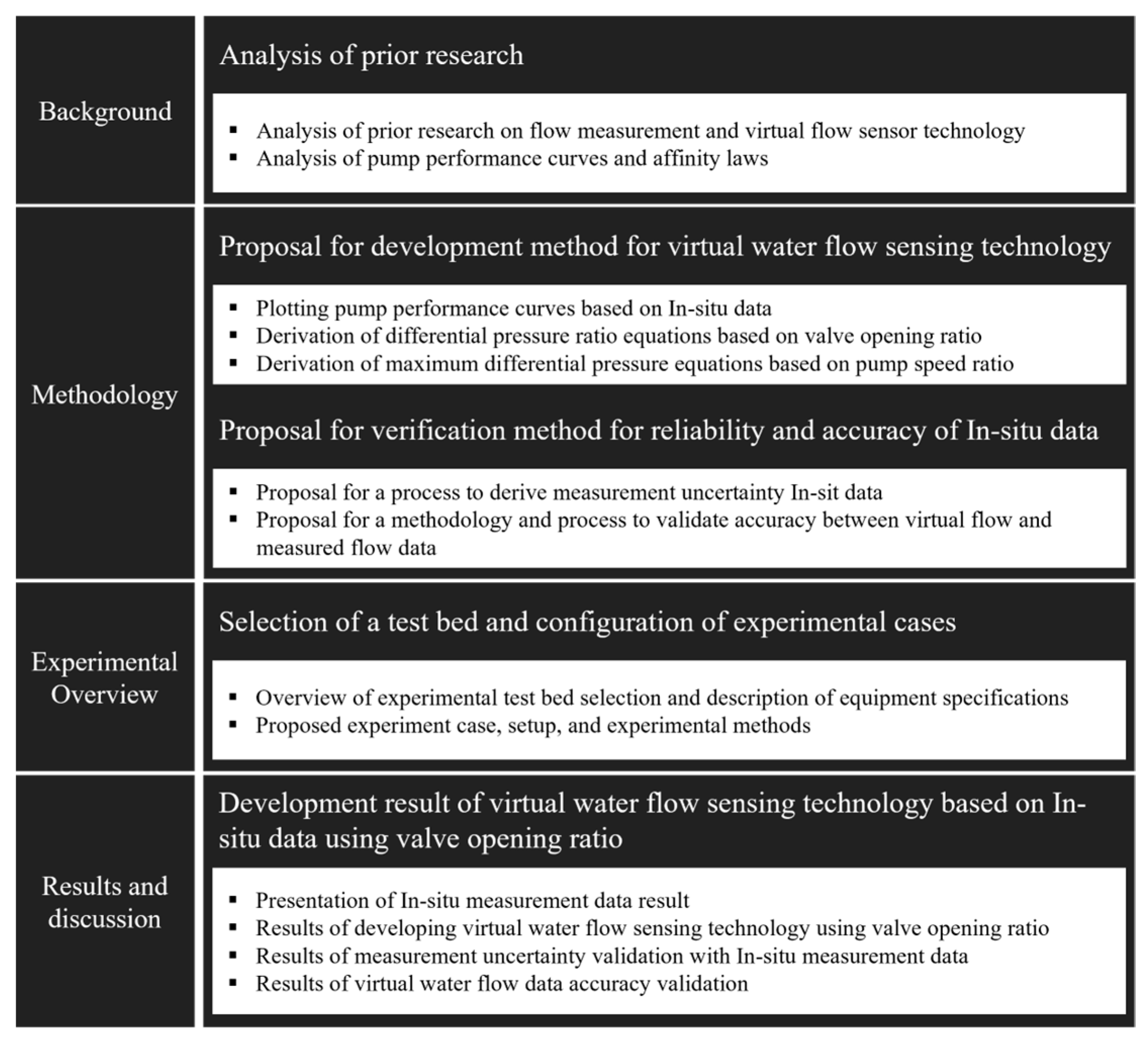
This subsection introduces the importance and efficiency of flow measurement, as well as an analysis of prior research related to the development of virtual flow-sensing technology utilizing pump speed and valve opening rate. The following research studies highlight advancements in energy efficiency through flow measurement and the development of virtual flow-sensing technology.

Table 1. Relative research analysis of flow rate measurement and virtual flow technology.

Reference	Main Research Focus	Results/Impact
Jung et al., 2014 [15]	Optimization of pump flow rate in geothermal heat pump systems.	Reduced pump energy consumption and operational cost savings.
Sarbu et al., 2015 [16]	Energy efficiency in district heating systems using variable-speed pumps.	Energy savings of 20% to 50% through dynamic flow control.
Shin et al., 2018 [17]	Flow rate control in primary geothermal heat pump systems.	Improved system efficiency and stability.
Wang et al., 2021 [18]	Optimization of secondary centrifugal pump flow control.	Enhanced energy efficiency and system stability.
Swamy et al., 2012 [19]	Virtual chilled-water flow meter for HVAC systems.	Cost-effective solution for accurate flow estimation.
Song et al., 2012 [20]	Impact of uncertainty on virtual flow measurement accuracy.	Improved reliability and accuracy in virtual flow sensing.

summarizes the authors, main research focus, and results/impact.

Jung et al. [15] evaluated the impact of pump flow rate changes on the energy performance of geothermal heat pump systems. Their optimization experiments demonstrated that adjusting the flow rate could reduce pump energy consumption and improve the system’s coefficient of performance (COP). The research showed that controlling the flow rate enhanced system efficiency and led to operational cost savings.

Sarbu et al. [16] proposed a method for enhancing energy efficiency in district heating systems by using optimized pump systems. The research focused on the use of variable-speed pumps to control flow rates and adjust pump speeds according to heating demand. Their findings demonstrated that adjusting pump speed could result in energy savings ranging from 20% to 50%.

Shin et al. [17] proposed a method for controlling the flow rate of primary pumps in geothermal heat pump systems to enhance system efficiency. This method adjusts the flow rate in real time according to load demands, thereby optimizing energy usage. Their research demonstrated that maintaining an appropriate flow rate contributes to both energy savings and improved system stability.

Wang et al. [18] introduced an optimization strategy for secondary centrifugal pump flow control by applying adaptive control technology. Using control algorithms, the system dynamically adjusts to determine the optimal water flow rate under varying operating conditions, thereby increasing energy efficiency. The research included the design and implementation of the control system, supported by experiments that validated its effectiveness in saving energy while maintaining system stability during flow control.

Swamy et al. [19] developed a virtual chilled-water flow meter for HVAC systems. They proposed a method for indirectly calculating chilled-water flow by measuring differential pressure and valve stem position. This approach allows for accurate flow estimation without direct measurement, providing an efficient solution for system monitoring.

Song et al. [20] analyzed the impact of uncertainty in system parameters on the accuracy of virtual water flow measurements. The research emphasized the importance of considering these uncertainties when using virtual sensors for building energy monitoring. It analyzed how various factors, such as sensor inaccuracies and system characteristics, propagate through the measurement process and proposed methods to improve measurement reliability.

2. Methodology

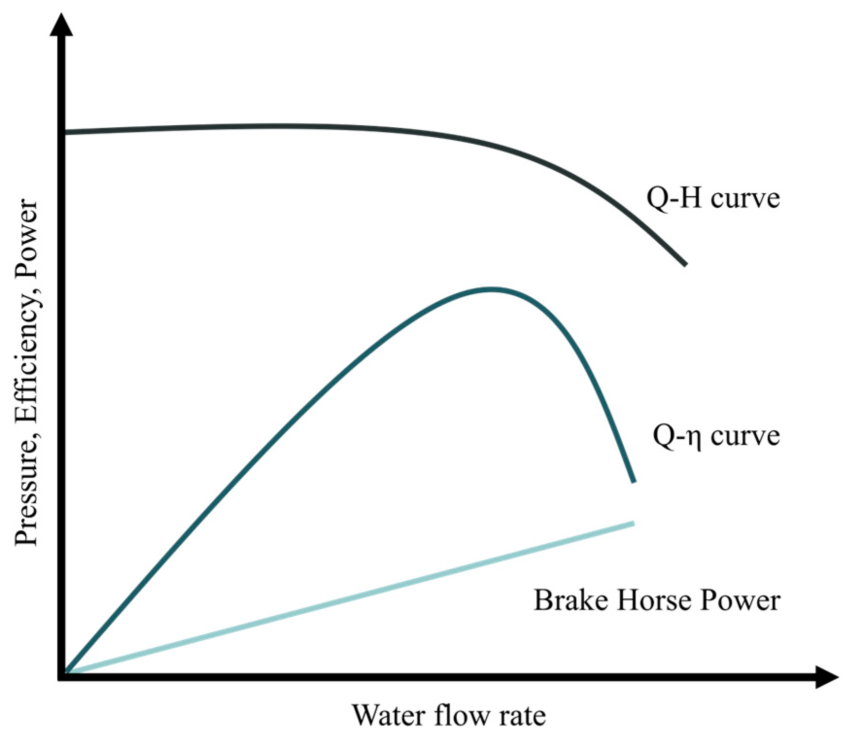
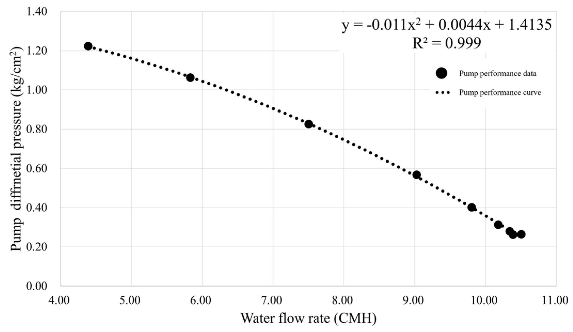
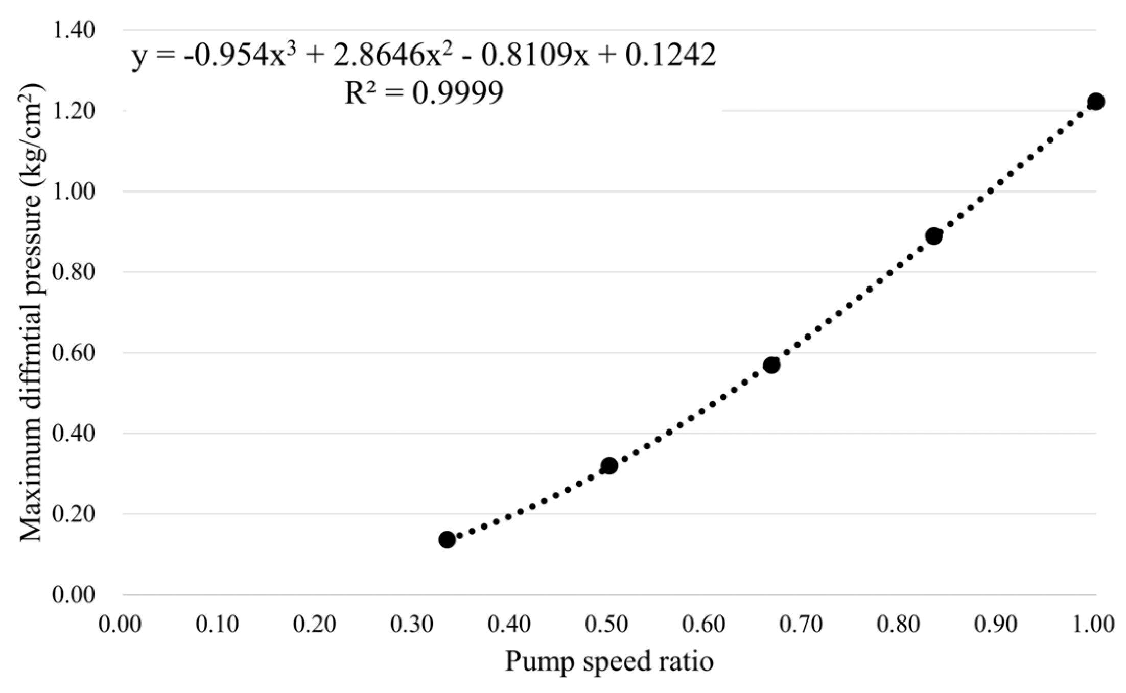
2.1. Pump Performance Curve

To accurately predict the virtual water flow rate in a circulating water pipe, it is crucial to understand the interdependencies among key parameters, such as water flow rate and pressure differential (DP). A useful framework for this analysis is the application of similarity laws [21]. Specifically, the pump similarity law provides a foundation for understanding how pump performance varies with changes in all speeds. According to this principle, proportional relationships must be maintained between a prototype and its model in order to ensure accurate predictions of performance. In the context of pump similarity, this law establishes proportional relationships between variables such as water flow rate, pressure differential, and power, all of which are influenced by the pump at all speeds [22]. The relationships between pump speed, water flow rate, pressure, and power based on similarity laws are expressed in Equations (1) through (3). Here, $N_{s,1}$ and $N_{s,2}$ indicates the pump speed, $Q_{s,1}$ and $Q_{s,2 }$ indicates the water flow rate, $H_{s,1}$ and $H_{s,2 }$ indicates the pump pressure, and $P_{s,1, s.2}$ indicates the pump power.

$$Q_{s,1}=Q_{s,2}\times \left({\displaystyle \frac{N_{s,1}}{N_{s,2}}}\right)$$

(1)

$$H_{s,1}=H_{s,2}\times {\left({\displaystyle \frac{N_{s,1}}{N_{s,2}}}\right)}^2$$

(2)

$$P_{s,1}=P_{s,2}\times {\left({\displaystyle \frac{N_{s,1}}{N_{s,2}}}\right)}^3$$

(3)

The pump performance curve serves as a graphical tool for evaluating the operating characteristics of a pump. As depicted in Figure 2, the horizontal axis represents the water flow rate, while the vertical axis displays variables such as pressure differential, power, and efficiency. Depending on which variable is plotted on the vertical axis, the performance curves can be categorized into Q-H (water flow rate and pressure), Q-P (water flow rate and power), or Q-η (water flow rate and efficiency). When the pump operates at a constant for all speeds, the performance curve can be expressed as a quadratic function based on the similarity principle, as outlined in Equation (4). By rearranging this equation using the quadratic formula, we can express the virtual water flow rate based on the pump performance curve in terms of pressure differential and all pump speeds, as outlined in Equation (5) [23]. Here, $Q_{water}$ indicates the water flow rate, while $a$, $b$, and $c$ are the pump performance curve coefficients from the Q-H curve. $H_{pump}$ indicates the pump differential pressure, and $\omega$ indicates the specific operating pump speed relative to the maximum pump speed.

$$H_{pump}=a{\left(Q_{water}\right)}^2+b\omega Q_{water}+c{\omega }^2$$

(4)

$$Q_{water} = {\displaystyle \frac{-b\omega \pm \sqrt{(b\omega {)}^2-4a(c{\omega }^2-H_{pump})}}{2a}}$$

(5)

2.2. Development Method for Virtual Water Flow-Sensing Technology

The water flow rate in HVAC systems is influenced by several factors, including the valve opening degree, differential pressure, and pump speed. The development of virtual flow-sensing technology, utilizing in situ measurements of valve opening and pump speed as independent variables, proceeds through the following steps:

Step 1: A test setup that includes a flow meter capable of measuring the water flow rate within the piping system is constructed, along with a control system that can regulate and monitor both the valve opening degree and pump speed. Additionally, pressure gauges are to be installed for measuring the pressure before and after the pump.

Step 2: To derive the pump performance curve from the measured discharge and return pressures, as well as flow data, the following experiment is performed: Set the pump to its maximum speed and systematically adjust the valve opening degree while simultaneously recording the pressure differential across the pump and the water flow rate. Utilize the collected pressure and flow data to construct the pump performance curve, as detailed in Equation (6) [23].

$${\mathrm{H}}_{\mathrm{f}}={{\mathrm{a}\mathrm{Q}}_{\mathrm{f}}}^2+{\mathrm{b}\mathrm{Q}}_{\mathrm{f}}+\mathrm{c}$$

(6)

As shown in Figure 3, the water flow rate and the pressure difference across the pump vary according to the valve opening degree and the pump speed [23]. The relationship between water flow rate and pressure difference as pump speed changes can be expressed using the affinity laws, which are represented by Equation (7). By combining this with Equation (6), the pump performance curve-based virtual water flow rate relationship can be derived as shown in Equation (8).

$${\displaystyle \frac{\mathrm{H}}{{\mathrm{H}}_{\mathrm{f}}}}=({\displaystyle \frac{\mathrm{N}}{{\mathrm{N}}_{\mathrm{f}}}}{)}^2=({\displaystyle \frac{\mathrm{Q}}{{\mathrm{Q}}_{\mathrm{f}}}}{)}^2={\mathsf{\omega }}^2$$

(7)

$$\mathrm{Q} = {\displaystyle \frac{-\mathrm{b}\mathsf{\omega }\pm \sqrt{(\mathrm{b}\mathsf{\omega }{)}^2-4\mathrm{a}(\mathrm{c}{\mathsf{\omega }}^2-\mathrm{H})}}{2\mathrm{a}}}$$

(8)

Step 3: Using Equation (5), the water flow rate within the HVAC system piping can be determined by utilizing the pressure differential across the pump and the pump speed as the independent variables. However, the calculation of the water flow rate requires additional pressure sensors. In buildings with multiple pipe branches and numerous valves, this would necessitate the installation of pressure sensors at each measurement point, which would significantly increase costs. To address this challenge, we propose substituting the pump’s discharge and return pressure sensors with one of the existing flow control elements, the valve opening degree, as an independent variable. By analyzing the relationship between the valve opening degree and the pressure differential, we aim to leverage this information for accurate flow estimation. To examine the relationship between valve opening degree and pressure differential ratio, experiments were conducted where the pump was fixed at maximum speed and the valve opening degree was varied. This experimentation led to the development of a formula, presented in Equation (9), in which the valve opening degree serves as the independent variable. The pressure differential ratio, defined in Equation (10), represents the ratio between the pressure differential at a partial valve opening and the pressure differential at the maximum valve opening. Based on the experimental data, a relationship was derived that describes the pressure differential ratio with the valve opening degree as an independent variable.

Here, $\mathsf{\beta }$ indicates the specific operating pump differential pressure relative to the maximum pump differential pressure, ${\mathrm{B}}_{\mathrm{n}}$ is the coefficient of the differential pressure ratio equation, and ${\mathsf{\alpha }}^{\mathrm{i}-n}$ indicates the valve opening rate. ${\mathrm{H}}_{\mathrm{m}\mathrm{a}\mathrm{x}}$ indicates the maximum pump differential pressure under the condition of the minimum valve opening rate.

$$\mathsf{\beta }={\mathrm{B}}_1{\mathsf{\alpha }}^{\mathrm{i}}+{\mathrm{B}}_2{\mathsf{\alpha }}^{\mathrm{i}-1}+\cdots +{\mathrm{B}}_{\mathrm{n}}$$

(9)

$$\mathsf{\beta }=\mathrm{H}/{\mathrm{H}}_{\mathrm{m}\mathrm{a}\mathrm{x}}$$

(10)

Step 4: By fixing the valve opening at its minimum degree and varying the pump speed, the pressure and water flow rate data were measured. Using these data, an equation for the maximum pressure difference with pump speed as the independent variable was derived, as shown in Equation (11). Here, ${\mathrm{C}}_n$ indicates the coefficient in the equation for deriving the maximum differential pressure.

$${\mathrm{H}}_{\mathrm{m}\mathrm{a}\mathrm{x}}={\mathrm{C}}_1{\mathsf{\omega }}^{\mathrm{l}}+{\mathrm{C}}_2{\mathsf{\omega }}^{\mathrm{l}-1}+\cdots +{\mathrm{C}}_{\mathrm{m}}$$

(11)

Using Equations (9)–(11), a differential pressure equation was derived as Equation (12), where both valve opening percentage and pump speed are treated as independent variables.

$$\mathrm{H}=\mathsf{\beta }{\mathrm{H}}_{\mathrm{m}\mathrm{a}\mathrm{x}}=({\mathrm{B}}_1{\mathsf{\alpha }}^{\mathrm{i}}+{\mathrm{B}}_2{\mathsf{\alpha }}^{\mathrm{i}-1}+\cdots +{\mathrm{B}}_{\mathrm{n}})({\mathrm{C}}_1{\mathsf{\omega }}^{\mathrm{l}}+\mathrm{C}{\mathsf{\omega }}^{\mathrm{l}-1}+\cdots +{\mathrm{C}}_{\mathrm{m}})$$

(12)

By combining Equations (8) and (12), the final virtual flow formula, expressed as Equation (13), is derived. This formula enables the estimation of fluid flow within the HVAC system’s piping based purely on the valve opening percentage and the pump speed, eliminating the need for direct pressure measurements.

$$\mathrm{Q}={\displaystyle \frac{-\mathrm{b}\mathsf{\omega }\pm \sqrt{(\mathrm{b}\mathsf{\omega }{)}^2-4\mathrm{a}(\mathrm{c}{\mathsf{\omega }}^2-({\mathrm{B}}_1{\mathsf{\alpha }}^{\mathrm{i}}+{\mathrm{B}}_2{\mathsf{\alpha }}^{\mathrm{i}-1}+\cdots +{\mathrm{B}}_{\mathrm{n}})({\mathrm{C}}_1{\mathsf{\omega }}^{\mathrm{l}}+\mathrm{C}{\mathsf{\omega }}^{\mathrm{l}-1}+\cdots +{\mathrm{C}}_{\mathrm{m}}))}}{2\mathrm{a}}}$$

(13)

2.3. Verification Method for Reliability of In Situ Data

The in situ data measurement process is inherently subject to uncertainty, which arises from factors such as the number of repetitions and the accuracy of the equipment employed. To mitigate the impact of these uncertainties and assess the reliability of the measurements, the following procedures are implemented to derive the measurement uncertainty, as illustrated in Figure 4.

Step 1: The developed virtual flow equation is designated as the measurement function, establishing the dependent relationships among the variables to be measured.

Step 2: The standard uncertainty and degrees of freedom for each independent variable are determined. At this stage, Type A uncertainty is derived from repeated measurements, while Type B uncertainty stems from the accuracy of the measuring equipment. Type A uncertainty is calculated by dividing the standard deviation of the measured values by the number of measurements, whereas Type B uncertainty is obtained through the resolution of the measuring device [24].

Step 3: To quantitatively express how changes in independent variables affect the results, sensitivity coefficients are calculated using the law of propagation of uncertainty. These coefficients can be derived by performing partial differentiation of the measurement function [24].

Step 4: Using the Root Sum Square Method (RSSM), as shown in Equation (14), the combined standard uncertainty is obtained from the Type A and Type B uncertainties and the sensitivity coefficients [25]. Here, $u(z)$ indicates the combined standard uncertainty, ${\displaystyle \frac{\partial f}{\partial x_i}}$ indicates the sensitivity coefficient, and $u_i$ indicates the individual uncertainty (either A or B).

$$u(z)=\sqrt{\sum _{i=1}^n{\left({\displaystyle \frac{\partial f}{\partial x_i}}\times u_i\right)}^2}$$

(14)

Step 5: Effective degrees of freedom are determined using the Welch–Satterthwaite equation, as illustrated in Equation (15) [26]. Here, ${\mathrm{v}}_{\mathrm{e}\mathrm{f}\mathrm{f}}$ indicates the effective degrees of freedom, ${\mathrm{v}}_{\mathrm{i}}$ indicates the degrees of freedom of the $i$-th uncertainty term, and $N$ indicates the total number of uncertainty terms contributing to the combined standard uncertainty.

$${\mathrm{v}}_{\mathrm{e}\mathrm{f}\mathrm{f}}={\displaystyle \frac{{{\mathrm{u}}_{\mathrm{c}}}^4}{{\sum }_{\mathrm{i}=1}^N(\frac{{\left(c_i{u}_i\right)}^4}{{\mathrm{v}}_{\mathrm{i}}})}}$$

(15)

Step 6: The inclusion factor k is determined through the effective degrees of freedom and the t-distribution table. According to the t-distribution table, if the effective degrees of freedom are sufficiently large, the inclusion factor k is equal to 2. [27] By multiplying the inclusion factor with the combined standard uncertainty, the expanded uncertainty is derived, completing the measurement uncertainty validation process.

2.4. Verification Method for Accuracy of Virtual Water Flow-Sensing Technology

The virtual flow meter, which predicts the water flow rate within HVAC system piping, is calculated using various independent variables. However, measurement sensors can introduce errors in these independent variables, potentially leading to discrepancies between the actual and virtually measured water flow rate [28]. To analyze these errors and derive an accurate virtual flow equation, several statistical methods are employed, including absolute error (AE), relative error (RE), Root Mean Square Error (RMSE), Normalized Root Mean Square Error (nRMSE), Coefficient of Variation of RMSE (CvRMSE), Mean Bias Error (MBE), and coefficient of determination (R²).

RMSE is a statistical metric used to assess the difference between predicted and actual values; a smaller RMSE indicates better model performance [29]. nRMSE evaluates relative error by dividing RMSE by the range of the actual data [30]. CvRMSE normalizes RMSE using the means of the actual values to assess relative predictive accuracy [31]. According to the International Performance Measurement and Verification Protocol (IPMVP) presented by EVO, a CvRMSE value below 10% suggests that the predictive model is performing well [32]. MBE measures the bias between the model’s predictions and the actual values, indicating whether the predictions tend to overestimate or underestimate the true values. A value of MBE approaching zero indicates that the predictions align closely with the actual data [33]. R² is a statistical metric used to determine the goodness of fit of the model; values closer to 1 indicate a stronger correlation between predicted and actual values [31]. To validate the accuracy of the virtual flow equation described above, the following steps are undertaken:

Step 1: Establish a test bed that includes a flow meter capable of measuring water flow rate changes in response to variations in valve opening and pump speed, along with a system to adjust these parameters.

Step 2: Collect water flow rate data by altering the valve opening and pump speed.

Step 3: Assess the accuracy of the virtual water flow rate by comparing it to the measured water flow rate, using Equations (16) through (22). Here, ${\mathrm{x}}_{\mathrm{m}\mathrm{e}\mathrm{a}\mathrm{s}}$ indicates the measured water flow rate, ${\mathrm{x}}_{\mathrm{v}\mathrm{i}\mathrm{r}}$ indicates the predicted water flow rate, and $\overline{\mathrm{x}}$ indicates the average of the measured water flow rate.

$$\mathrm{A}\mathrm{E}={\mathrm{x}}_{\mathrm{m}\mathrm{e}\mathrm{a}\mathrm{s}}-{\mathrm{x}}_{\mathrm{v}\mathrm{i}\mathrm{r}}$$

(16)

$$\mathrm{R}\mathrm{E}={\displaystyle \frac{{\mathrm{x}}_{\mathrm{m}\mathrm{e}\mathrm{a}\mathrm{s}}-{\mathrm{x}}_{\mathrm{v}\mathrm{i}\mathrm{r}}}{{\mathrm{x}}_{\mathrm{m}\mathrm{e}\mathrm{a}\mathrm{s}}}}\times 100$$

(17)

$$\mathrm{RMSE}=\sqrt{{\displaystyle \frac{{\sum }_1^{\mathrm{n}}({\mathrm{x}}_{\mathrm{m}\mathrm{e}\mathrm{a}\mathrm{s}}-{\mathrm{x}}_{\mathrm{v}\mathrm{i}\mathrm{r}}{)}^2}{\mathrm{n}}}}$$

(18)

$$\mathrm{n}\mathrm{RMSE}={\displaystyle \frac{\sqrt{\frac{{\sum }_1^{\mathrm{n}}({\mathrm{x}}_{\mathrm{m}\mathrm{e}\mathrm{a}\mathrm{s}}-{\mathrm{x}}_{\mathrm{v}\mathrm{i}\mathrm{r}}{)}^2}{\mathrm{n}}}}{{\mathrm{x}}_{\mathrm{m}\mathrm{e}\mathrm{a}\mathrm{s}.\mathrm{m}\mathrm{a}\mathrm{x}}-{\mathrm{x}}_{\mathrm{m}\mathrm{e}\mathrm{a}\mathrm{s}.\mathrm{m}\mathrm{i}\mathrm{n}}}}$$

(19)

$$\mathrm{C}\mathrm{v}\mathrm{R}\mathrm{M}\mathrm{S}\mathrm{E}={\displaystyle \frac{\mathrm{RM}\mathrm{SE}}{\overline{\mathrm{x}}}}\times 100$$

(20)

$$\mathrm{M}\mathrm{B}\mathrm{E}={\displaystyle \frac{1}{\mathrm{n}}}\sum _{\mathrm{i}=1}^{\mathrm{n}}({\mathrm{x}}_{\mathrm{m}\mathrm{e}\mathrm{a}\mathrm{s}}-{\mathrm{x}}_{\mathrm{v}\mathrm{i}\mathrm{r}})$$

(21)

$${\mathrm{R}}^2=1-{\displaystyle \frac{{\sum }_1^{\mathrm{n}}({\mathrm{x}}_{\mathrm{m}\mathrm{e}\mathrm{a}\mathrm{s}}-{\mathrm{x}}_{\mathrm{v}\mathrm{i}\mathrm{r}}{)}^2}{{\sum }_1^{\mathrm{n}}({\mathrm{x}}_{\mathrm{v}\mathrm{i}\mathrm{r}}{)}^2}}$$

(22)

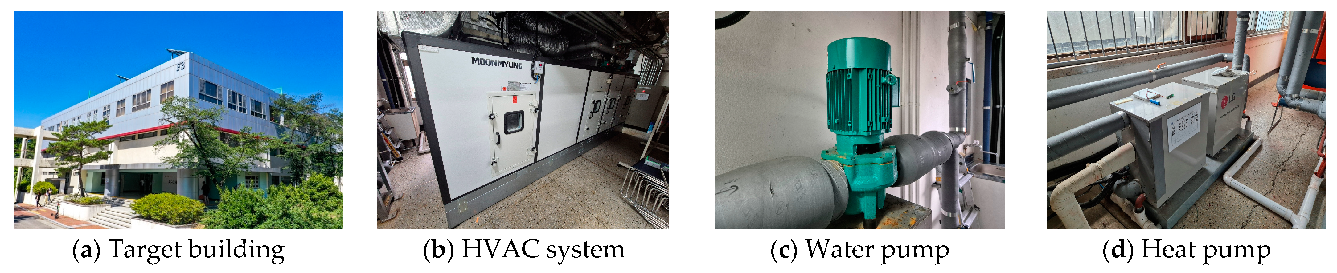
3. Experimental Overview

3.1. Selection of Test Bed

In this research, the objective is to develop a virtual flow equation using valve opening rate and all pump speeds as independent variables. The experimental test bed is established in a university laboratory, which is equipped with an HVAC multi-loop system. This HVAC system comprises an inline pump for water circulation, valves controlled by a Building Automation System (BAS), and a heat pump that manages discharge temperature through heat exchange with the refrigerant. Figure 5 illustrates the target building and the installed HVAC system, while

Table 2. Target space overview.

Category	Content
Use	Laboratory
Floor area	35.5 m2
Height	3.4 m
Volume	120 m3

provides an overview of the system. Flow measurements in the test bed were performed using an ultrasonic flow meter that employs the Z method, with the specifications of the ultrasonic flow meter outlined in

Table 3. Pump and ultrasonic flow meter specification.

Equipment	Category	Specification
Pump	Handling liquid	0~120 °C (pH 6~8)
	Water flow rate	0~480 m3/h
	Head	0~55 m
	Motor power	1~100 HP
	Full pump speed	60 Hz
Ultrasonic flow meter	Measuring category	Water flow rate
	Measuring range	0~±15 m/s
	Accuracy	±1%

.

3.2. Experimental Case Setup and Methodology

This research aims to develop a virtual water flow rate prediction technique with pump speed and valve opening rate as independent variables. According to the methodology outlined earlier, the initial conditions for the virtual water flow rate prediction technique are based on the pump speed and valve opening rate.

Generally, during automatic control operation, the pump operates at a constant speed of 60 Hz, and the valve operates between a maximum of 100% and a minimum of 20%. Additionally, the boundary conditions for the water flow rate prediction are defined by the heat pump outlet temperature, the density of water, and the pipe’s outer diameter and thickness. The initial and boundary conditions for the experiment are summarized in

Table 4. Initial conditions and boundary conditions.

Parameter	Initial Condition	Parameter	Boundary Condition
Pump speed	60 Hz (Maximum)	Heat pump outlet temperature	9.4~16.9 °C
		Water density	999.0~999.1 kg/m3
Valve opening rate	100% (Maximum) ~20% (Minimum)	Pipe outer diameter	41.28 mm
		Pipe wall thickness	1.24 mm

.

The experimental cases based on these conditions are presented in

Table 5. Experiment case.

Case		Pump Speed (Hz)	Valve Opening Rate (%)
1	1	60	100
	2		90
	3		80
	4		70
	5		60
	6		50
	7		40
	8		30
	9		20
2	1	50	20%
	2	40
	3	30
	4	20

. The pump speed starts at 60 Hz (maximum speed) and is gradually reduced in 10 Hz increments until reaching 20 Hz. The valve opening rate starts at 100% (maximum opening) and is gradually reduced in 10% increments until reaching 20%. Case 1 involves fixing the pump speed at its maximum and varying the valve opening rate to analyze the pressure differential ratio. Case 2 focuses on fixing the valve opening rate at its minimum and varying the pump speed to determine the maximum pressure differential.

In this research, an ultrasonic flow meter for measuring water flow and pressure gauges for measuring the pump discharge and return pressures were used as part of the experimental setup. The ultrasonic flow meter was installed in the piping before the water enters the cooling coil in the HVAC system, after passing through the pump and heat exchanger. The pressure gauges were installed at both the pump discharge and return sides. The water flow rate and pump discharge and return pressures for each experimental case were measured for 10 min, with data collected every minute. The pump speed and valve opening rate were manually controlled through the BAS installed in the test bed, and the pressures at the pump discharge and return were monitored and recorded via the BAS. The schematic diagram of the ultrasonic flow meter and pressure gauge measurement locations, as well as the system within the test bed, is shown in Figure 6.

4. Results and Discussion

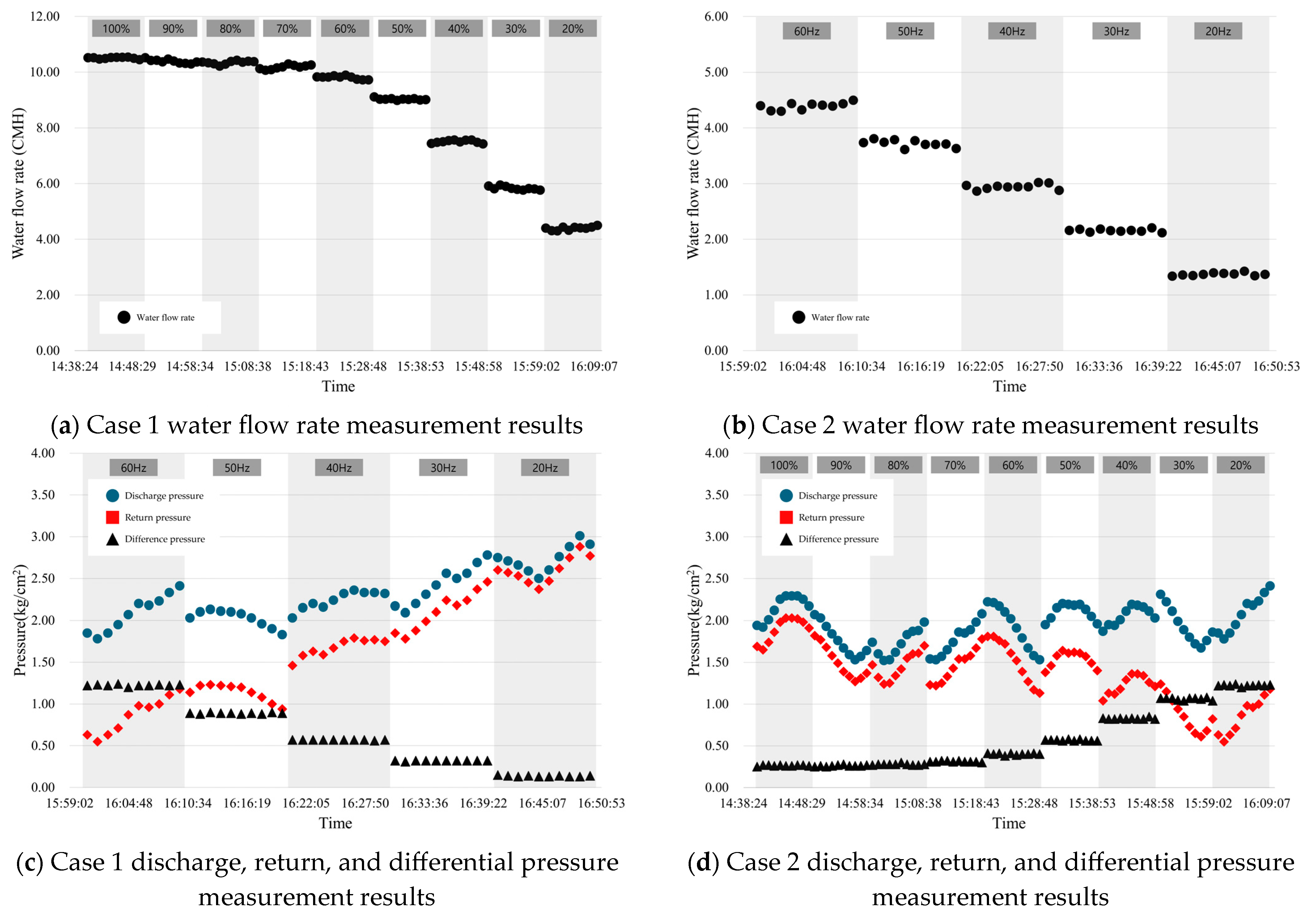
4.1. Results of In Situ Data by Case

To determine the water flow rate in response to variations in all pump speeds and valve opening rates for each experimental scenario, an ultrasonic flow meter was used to measure the water flow rate, while pressure data were obtained through Building Automation System (BAS) readings. The data collected by adjusting the valve opening rate at the maximum pump speed in Case 1 are presented in

Table 6. Measurement data at full speed for Case 1.

Case		Pump Speed (Hz)	Valve Opening Rate (%)	Water Flow Rate (CMH)	DP (kg/cm2)
1	1	60	100	10.51	0.26
	2		90	10.39	0.26
	3		80	10.34	0.28
	4		70	10.18	0.31
	5		60	9.81	0.40
	6		50	9.03	0.57
	7		40	7.50	0.83
	8		30	5.83	1.06
	9		20	4.39	1.22

, and the corresponding variations in water flow rate, discharge pressure, return pressure, and pressure differential are depicted in Figure 7a,b. When the valve opening rate was altered at the maximum pump speed, the water flow rate at full valve opening was measured at 10.51 CMH, with a pressure differential of 0.26 kg/cm² across the pump. At the minimum valve opening, the water flow rate decreased to 4.39 CMH, with a corresponding pressure differential of 1.22 kg/cm² across the pump. In Case 2, the data obtained by varying the pump speed at the minimum valve opening rate are shown in

Table 7. Measurement data at lowest valve opening rate for Case 2.

Case		Pump Speed (Hz)	Valve Opening Rate (%)	Water Flow Rate (CMH)	DP (kg/cm2)
2	1	50	20	3.72	0.89
	2	40		2.94	0.57
	3	30		2.16	0.32
	4	20		1.37	0.14

, with the resulting changes in water flow rate, discharge pressure, return pressure, and pressure differential illustrated in Figure 7c,d. When the pump speed was varied at the minimum valve opening, the water flow rate was 4.39 CMH with a pressure differential of 1.22 kg/cm² at the maximum pump speed. Conversely, at the lowest pump speed, the water flow rate decreased to 1.37 CMH, with a pressure differential of 0.14 kg/cm².

4.2. Development of Water Virtual Flow-Sensing Technology Using Valve Opening Rate

Using the water flow rate and pressure differential data from Case 1 (varying the valve opening rate at the maximum pump speed), the pump performance curve was derived as shown in Figure 8. The in situ measured pump performance curve can be represented as a quadratic function, as expressed in Equation (23).

$${\mathrm{H}}_{\mathrm{f}}=-0.011{{\mathrm{Q}}_{\mathrm{f}}}^2+0.0044{\mathrm{Q}}_{\mathrm{f}}+1.4135$$

(23)

Equation (23) represents the pump performance curve at the maximum pump speed. This curve does not apply uniformly to other pump speeds. However, using the earlier Equation (7), the pump performance curve for different pump speeds can be plotted as shown in Equation (24). By rearranging this equation using the quadratic formula, the water flow rate can be expressed as shown in Equation (25).

$$\mathrm{H}=-0.011Q^2+0.0044\omega \mathrm{Q}+1.4135{\omega }^2$$

(24)

$$\mathrm{Q} = 0.2\mathsf{\omega }+{\displaystyle \frac{\sqrt[]{0.06221{\mathsf{\omega }}^2-0.044\mathrm{H}}}{0.022}}$$

(25)

To derive the pressure differential ratio based on variations in valve opening rate, the pressure differential data from Case 1 was analyzed, as depicted in Figure 9. The relationship between valve opening rate and pressure differential ratio, shown in Figure 9a, exhibited consistent trends corresponding to changes in pump speed. When this relationship was modeled as a sixth-degree polynomial, a strong correlation was observed, with an R² value of 0.9999. This confirmed the representativeness of the valve pressure differential ratio at a pump speed of 60 Hz. Consequently, Equation (26) was formulated as a sixth-degree polynomial, which resulted in an R² value of 0.999, further validating the accuracy of the model.

$$\mathsf{\beta }=46.22{\mathsf{\alpha }}^6-153.76{\mathsf{\alpha }}^5+190.96{\mathsf{\alpha }}^4-105.97{\mathsf{\alpha }}^3+24.427{\mathsf{\alpha }}^2-2.8547\mathsf{\alpha }+1.1845$$

(26)

By changing all of the pump speeds to the minimum valve opening rate and utilizing the measured difference pressure, the relationship between the pump’s full speed and maximum difference pressure was derived, as shown in Figure 10. The maximum difference pressure with variations in all pump speeds is represented as a third-degree curve in Equation (26), with an R² value of 0.9999.

$${\mathrm{H}}_{\mathrm{m}\mathrm{a}\mathrm{x}}=-0.954{\mathsf{\omega }}^3+2.8646{\mathsf{\omega }}^2-0.8109\mathsf{\omega }+0.1242$$

(27)

Using Equations (25)–(27), a virtual flow-sensing technology was developed that incorporates valve opening rate and all pump speeds as input variables.

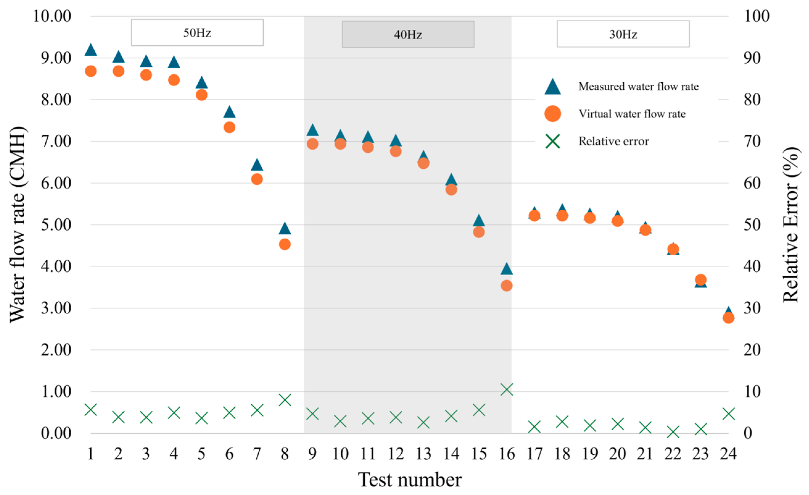
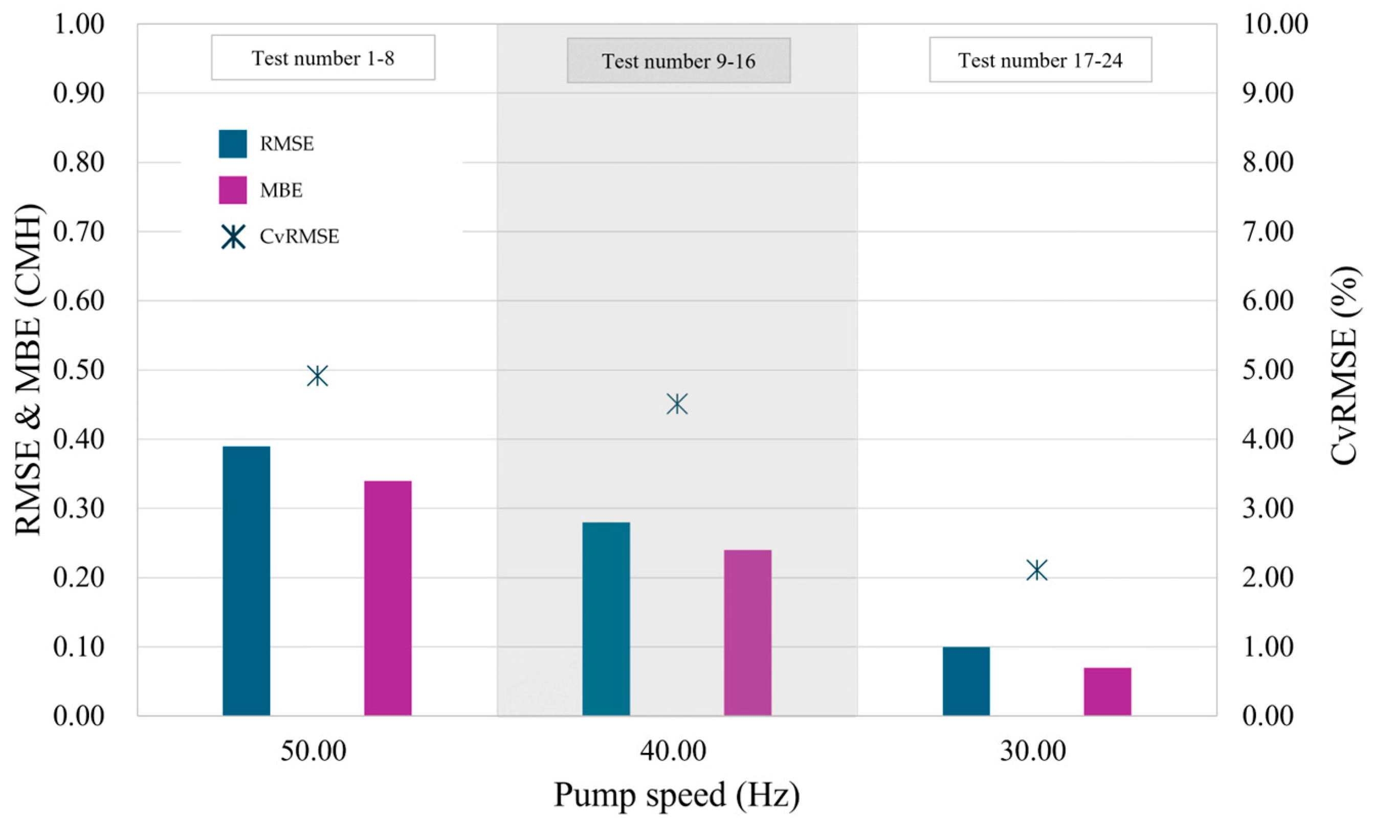
4.3. Validation Results of the Water Virtual Flow Meter

In Section 4.1 and Section 4.2, virtual flow-sensing technology was developed based on in situ data measurements. To validate the accuracy of this developed virtual flow-sensing technology, pump speeds were set to range from 50 Hz to 30 Hz in 10 Hz decrements, while valve opening rates were adjusted from 100% to 30% in 10% increments, forming the experimental test cases. Data on pump speed and valve opening rate were collected through the Building Automation System (BAS), while water flow rates were measured using an ultrasonic flow meter installed in the piping system. Measurements were taken every minute for a duration of 10 min. Additionally, to assess the reliability of the measured data, measurement uncertainty was quantified. The measurement quantity function utilized the developed virtual flow-sensing equations. Type A uncertainty evaluation was carried out to quantify errors arising from the measurement process, while Type B uncertainty evaluation focused on the errors associated with the measuring instruments. Type A uncertainty was derived from the data collected at one-minute intervals over the ten-minute measurement period, while Type B uncertainty was determined based on the resolution of the ultrasonic flow meter and pressure gauge. Sensitivity coefficients for each type of uncertainty were derived by calculating the partial derivatives of the virtual flow-sensing equations, with Type A degrees of freedom set to nine and Type B degrees of freedom considered infinite based on the equipment resolution. The combined uncertainty was calculated by incorporating Type A uncertainty, sensitivity coefficients, Type B uncertainty, and their respective sensitivity coefficients. Finally, the expanded uncertainty was determined using the effective degrees of freedom. The measurement uncertainty for each experimental case is presented in

Table 8. Measurement uncertainty of experiment case.

Case		Type A Uncertainty (CMH)	Type B Water Flow Rate Uncertainty (CMH)	Type B DP Uncertainty (kg/cm2)	Combined Standard Uncertainty (CMH)	Expanded Uncertainty (CMH)
1	1	0.010	0.026	0.058	0.059	0.117
	2	0.022	0.026		0.062	0.124
	3	0.023	0.026		0.061	0.122
	4	0.023	0.025		0.062	0.124
	5	0.018	0.025		0.061	0.121
	6	0.011	0.023		0.059	0.118
	7	0.016	0.019		0.060	0.120
	8	0.020	0.015		0.061	0.122
	9	0.020	0.011		0.061	0.122
2	1	0.020	0.009	0.058	0.060	0.120
	2	0.016	0.007		0.058	0.117
	3	0.008	0.005		0.058	0.117
	4	0.009	0.001		0.058	0.117

, and the measurement uncertainty corresponding to each test case is provided in

Table 9. Measurement uncertainty of test number.

Test Number	Type A Uncertainty (CMH)	Type B Water Flow Rate Uncertainty (CMH)	Type B DP Uncertainty (kg/cm2)	Combined Standard Uncertainty (CMH)	Expanded Uncertainty (CMH)
1	0.020	0.023	0.058	0.061	0.122
2	0.015	0.023		0.060	0.119
3	0.023	0.022		0.062	0.124
4	0.019	0.022		0.061	0.122
5	0.014	0.021		0.059	0.119
6	0.022	0.019		0.062	0.124
7	0.011	0.016		0.059	0.118
8	0.019	0.012		0.061	0.121
9	0.017	0.018	0.058	0.060	0.120
10	0.018	0.018		0.061	0.121
11	0.017	0.018		0.060	0.120
12	0.016	0.018		0.060	0.120
13	0.015	0.017		0.060	0.120
14	0.013	0.015		0.059	0.119
15	0.018	0.013		0.060	0.121
16	0.010	0.010		0.059	0.117
17	0.013	0.013	0.058	0.059	0.118
18	0.008	0.013		0.058	0.117
19	0.011	0.013		0.059	0.118
20	0.012	0.013		0.059	0.118
21	0.013	0.012		0.059	0.118
22	0.013	0.011		0.059	0.118
23	0.011	0.009		0.059	0.118
24	0.010	0.007		0.059	0.117

.

The results of the comparison between the derived virtual water flow rate and the measured data, including an analysis of errors based on all pump speeds and valve opening rates, are summarized in

Table 10. Error analysis results.

Test Number	Pump Speed (Hz)	Valve Opening Rate (%)	Measured Water Flow Rate (CMH)	Virtual Water Flow Rate (CMH)	Absolute Error (CMH)	Relative Error (%)
1	50	100	9.21	8.69	0.52	5.66
2		90	9.04	8.69	0.35	3.92
3		80	8.93	8.59	0.34	3.82
4		70	8.91	8.47	0.44	4.94
5		60	8.42	8.11	0.31	3.64
6		50	7.72	7.34	0.38	4.91
7		40	6.45	6.09	0.36	5.52
8		30	4.92	4.53	0.39	7.99
9	40	100	7.28	6.94	0.34	4.67
10		90	7.14	6.94	0.21	2.89
11		80	7.12	6.86	0.26	3.59
12		70	7.03	6.76	0.27	3.85
13		60	6.65	6.47	0.17	2.61
14		50	6.09	5.84	0.25	4.11
15		40	5.11	4.83	0.29	5.59
16		30	3.96	3.54	0.42	10.54
17	30	100	5.30	5.22	0.08	1.55
18		90	5.37	5.22	0.15	2.78
19		80	5.26	5.16	0.10	1.85
20		70	5.21	5.09	0.12	2.25
21		60	4.95	4.88	0.07	1.38
22		50	4.43	4.42	0.01	0.32
23		40	3.65	3.68	−0.04	−1.01
24		30	2.90	2.77	0.14	4.67

. Figure 11 illustrates the measured flow values, virtual flow values, and the corresponding relative errors for each experimental case. The absolute error ranged from a minimum of 0.01 CMH to a maximum of 0.52 CMH. Moreover, the relative error varied between 0.32% and 10.54%, with the highest relative errors observed at a valve opening rate of 30%, regardless of all of the pump speeds.

The validation results, derived from statistical analysis including RMSE, nRMSE, CvRMSE, and MBE, are presented in

Table 11. Verification value through statistical analysis.

Test Number	Pump Speed	RMSE (CMH)	MBE (CMH)	nRMSE (-)	CvRMSE (%)	R2 (-)
1–8	50	0.39	0.34	0.09	4.92	0.998
9–16	40	0.28	0.24	0.09	4.51	0.998
17–24	30	0.10	0.07	0.04	2.11	0.996

, with the performance indicators based on all pump speeds shown in Figure 12. The RMSE values were recorded as 0.39 CMH at 50 Hz, 0.28 CMH at 40 Hz, and 0.10 CMH at 30 Hz. MBE values were calculated as 0.34 CMH at 50 Hz, 0.24 CMH at 40 Hz, and 0.07 CMH at 30 Hz, indicating that the predictions are close to 0 CMH, thus confirming the excellent predictive accuracy of the virtual flow equation. The nRMSE values were found to be 0.09 at 50 Hz, 0.09 at 40 Hz, and 0.04 at 30 Hz, demonstrating minimal error in predictive performance. CvRMSE values were measured at 4.92% for 50 Hz, 4.51% for 40 Hz, and 2.11% for 30 Hz, all of which remained within the 10% threshold, further validating the appropriateness of the prediction model. Additionally, the coefficient of determination (R²) values were 0.998 at 50 Hz, 0.998 at 40 Hz, and 0.996 at 30 Hz, reflecting a high degree of agreement between the measured and virtual water flow rates.

5. Conclusions

This research developed a novel virtual flow-sensing technology that addresses the limitations of conventional flow sensors, enabling accurate flow measurements in buildings with multiple valves and complex piping systems. By utilizing this technology, it becomes possible to estimate water flow rates in real time without the need for extensive physical sensors at every point in the system, which is especially advantageous for large-scale or retrofit building projects. The research also established a practical methodology for virtual flow in situ measurement, which is directly applicable to real building systems, providing a scalable and cost-effective solution for flow monitoring. To develop a virtual water flow rate prediction technology with valve opening rate and pump speed as independent variables, two experimental cases were designed: Case 1, where the valve opening rate was varied at maximum pump speed, and Case 2, where the pump speed was varied at minimum valve opening rate. In Case 1, the water flow rate and differential pressure measurement data were used to derive an in situ-based performance curve. Additionally, the relationship between the valve opening rate ratio and the differential pressure ratio was analyzed to derive a differential pressure ratio equation with the valve opening rate ratio as an independent variable. In Case 2, water flow rate and differential pressure measurement data were used to derive the maximum differential pressure equation with the pump speed ratio as an independent variable. The differential pressure ratio was calculated by dividing a specific differential pressure by the maximum differential pressure at the same pump speed, and a new equation to calculate specific differential pressure was derived by solving the differential pressure ratio and maximum differential pressure equations. This equation was applied to the performance curve to develop the virtual water flow rate prediction technology with valve opening rate and pump speed as independent variables.

Additionally, it was confirmed that measurement errors can occur due to the number of measurements and the precision of the equipment, and these errors were verified through measurement uncertainty analysis. The measurement errors were found to be within the upper and lower bounds in all experimental cases. To assess the accuracy of water flow rate predictions at different pump speeds, the model’s performance was validated using absolute error, relative error, RMSE, MBE, nRMSE, CvRMSE, and R². The absolute error ranged from 0.01 CMH to 0.52 CMH, and the relative error varied from 0.32% to 10.54%. RMSE values were 0.39 CMH at 50 Hz, 0.28 CMH at 40 Hz, and 0.09 CMH at 30 Hz. MBE values were 0.34 CMH at 50 Hz, 0.24 CMH at 40 Hz, and 0.07 CMH at 30 Hz, indicating that the model’s predictions are very close to zero, confirming the excellent predictive performance of the virtual water flow rate model. The nRMSE values were 0.09 at 50 Hz, 0.09 at 40 Hz, and 0.04 at 30 Hz, showing minimal error in predictive performance. CvRMSE values were 4.92% at 50 Hz, 4.51% at 40 Hz, and 2.11% at 30 Hz, all within the 10% threshold, indicating that the prediction model is highly suitable. The coefficient of determination (R²) was 0.998 at 50 Hz, 0.998 at 40 Hz, and 0.996 at 30 Hz, demonstrating a high degree of agreement between the measured and predicted water flow rates.

References

1. Jung, R.B. A Study on the EU’s Response to the United Nations Framework Convention on Climate Change. Master’s Thesis, Hankuk University of Foreign Studies, Seoul, Republic of Korea, 2022. [Google Scholar]
2. Jeong, Y.S. Decomposition Analysis and Reduction Implementation Indicator of Greenhouse Gas Emission in Building Sector. J. Archit. Inst. Korea 2024, 40, 225–234. [Google Scholar]
3. Chae, Y.G. Legislative Challenges to Realize the 2050 Carbon Neutral Goal in Korea. Inha Law Rev. Inst. Leg. Stud. Inha Univ. 2022, 25, 63–99. [Google Scholar] [CrossRef]
4. UNFCCC. 2050 Carbon Neutral Strategy of the Republic of Korea; UNFCCC: Rio de Janeiro, Brazil, 2020. [Google Scholar]
5. Jin, J.T.; Seok, Y.J.; Cho, H.J.; Choi, S.G.; Hwang, D.K. Design of Chilled Water Temperature Condition of Large Temperature Differential Chiller for Saving Building Energy. Korean J. Air-Cond. Refrig. Eng. 2023, 35, 90–98. [Google Scholar]
6. Asim, N.; Badiei, M.; Mohammad, M.; Razali, H.; Rajabi, A.; Chin Haw, L.; Jameelah Ghazali, M. Sustainability of Heating, Ventilation and Air-Conditioning (HVAC) Systems in Buildings—An Overview. Int. J. Environ. Res. Public Health 2022, 19, 1016. [Google Scholar] [CrossRef]
7. Ministry of Trade, Industry and Energy. Statistics on Energy Use and Greenhouse Gas Emissions; Ministry of Trade, Industry and Energy: Sejong, Republic of Korea, 2019.
8. Lee, J.N.; Kim, Y.I.; Chung, K.S. Flow Control of a Centralized Cooling Plant for Energy Saving. J. Energy Eng. 2015, 24, 48–54. [Google Scholar] [CrossRef]
9. Kim, W.U. Experimental Study on the Water Flow Control of Partial Cooling/Heating Load in Water to Water Heat Pump. In Proceedings of the SAREK Annual Conference, Pyeongchang, Republic of Korea, 22–24 June 2022; pp. 303–306. [Google Scholar]
10. Lee, C.U.; Jin, S.; Do, S.L. Development of Virtual Sensor for Measurement of Heating Mass Flow Rate in Apartment Buildings using District Heating System. Proc. Korean Inst. Archit. Sci. Conf. 2021, 41, 632. [Google Scholar]
11. Wotzka, D.; Zmarzły, D. Low-Cost Device for Measuring Wastewater Flow Rate in Open Channels. Sensors 2024, 24, 6607. [Google Scholar] [CrossRef] [PubMed]
12. Choi, Y.W.; Yoon, S.M. Time Series Data Downscaling Method for Backup Virtual Sensor Performance Improvement in a Building Energy Sensor Network. Korean J. Air-Cond. Refrig. Eng. 2022, 34, 111–122. [Google Scholar]
13. Guzmán, C.H.; Carrera, J.L.; Durán, H.A.; Berumen, J.; Ortiz, A.A.; Guirette, O.A.; Arroyo, A.; Brizuela, J.A.; Gómez, F.; Blanco, A.; et al. Implementation of Virtual Sensors for Monitoring Temperature in Greenhouses Using CFD and Control. Sensors 2019, 19, 60. [Google Scholar] [CrossRef] [PubMed]
14. Li, H.; Yu, D.; Braun, J. A review of virtual sensing technology and application in building systems. HVAC&R Res. 2011, 17, 619–648. [Google Scholar]
15. Jung, Y.J.; Jo, J.H.; Kim, Y.S.; Cho, Y.H. A Study on the Geothermal Heat Pump System Performance Analysis according to Water Flow Rate Control of the Geothermal Water Circulation Pump. J. Korean Sol. Energy Soc. 2014, 34, 103–109. [Google Scholar] [CrossRef]
16. Sarbu, I.; Valea, E.S. Energy Savings Potential for Pumping Water in District Heating Stations. Sustainability 2015, 7, 5705–5719. [Google Scholar] [CrossRef]
17. Shin, J.H.; Cho, Y.H. Development of an Operating Method for Variable Water Flow Rate Control Method in Geothermal Heat Pump System. J. Korean Inst. Archit. Sustain. Environ. Build. Syst. 2018, 12, 510–518. [Google Scholar]
18. Wang, Y.; Zhang, H.; Han, Z.; Ni, X. Optimization design of centrifugal pump flow control system based on adaptive control. Processes 2021, 9, 1538. [Google Scholar] [CrossRef]
19. Swamy, S.; Song, L.; Wang, G. A Virtual Chilled-Water Flow Meter Development at Air Handling Unit Level. ASHRAE Trans. 2012, 118, 1013–1020. [Google Scholar]
20. Song, L.; Joo, I.; Wang, G. Uncertainty analysis of a virtual water flow measurement in building energy consumption monitoring. HVAC&R Res. 2012, 18, 997–1010. [Google Scholar]
21. Kim, Y.J.; Kim, P.H.; Lee, K.S.; Kim, B.H.; Chung, H.S.; Jeong, H.M. A Study on the Application of Pump Similarity Re-quirements according to Performance Variation of the Centrifugal Pump. In Proceedings of the KSME Spring Annual Meeting 2008, Jeongseon, Republic of Korea, 24–25 April 2008; p. 2614. [Google Scholar]
22. Liu, G. Development and Applications of Fan Airflow Station and Pump Water Flow Station in Heating, Ventilating, and Air-Conditioning (HVAC) Systems; University of Nebraska Lincoln ProQuest Dissertations Publishing: Lincoln, NE, USA, 2006; p. 3237050. [Google Scholar]
23. Kim, H.J.; Jae, H.J.; Cho, H.J. Development of Virtual Air Flow Sensor Using In-Situ Damper Performance Curve in VAV Terminal Unit. Energies 2019, 12, 4307. [Google Scholar] [CrossRef]
24. Wiora, J.; Wiora, A. Measurement Uncertainty Calculations for pH Value Obtained by an Ion-Selective Electrode. Sensors 2018, 18, 1915. [Google Scholar] [CrossRef]
25. Pham, H. A New Criterion for Model Selection. Mathematics 2019, 7, 1215. [Google Scholar] [CrossRef]
26. Pawłowski, E.; Szlachta, A.; Otomański, P. The Influence of Noise Level on the Value of Uncertainty in a Measurement System Containing an Analog-to-Digital Converter. Energies 2023, 16, 1060. [Google Scholar] [CrossRef]
27. ISO. Guide to the Expression of Uncertainty in Measurement; Aenor: Madrid, Spain, 1993. [Google Scholar]
28. Taylor, J.R. An Introduction to Error Analysis: The Study of Uncertainties in Physical Measurements, 2nd ed.; University Science Books: Sausalito, CA, USA, 1997. [Google Scholar]
29. Dobra, P.; Jósvai, J. Cumulative and Rolling Horizon Prediction of Overall Equipment Effectiveness (OEE) with Machine Learn-ing. Big Data Cogn. Comput. 2023, 7, 138. [Google Scholar] [CrossRef]
30. Abe, C.F.; Dias, J.B.; Notton, G.; Faggianelli, G.A. Experimental Application of Methods to Compute Solar Irradiance and Cell Temperature of Photovoltaic Modules. Sensors 2020, 20, 2490. [Google Scholar] [CrossRef] [PubMed]
31. Chen, Y.; Ye, Y.; Liu, J.; Zhang, L.; Li, W.; Mohtaram, S. Machine Learning Approach to Predict Building Thermal Load Consider-ing Feature Variable Dimensions: An Office Building Case Study. Buildings 2023, 13, 312. [Google Scholar] [CrossRef]
32. EVO. International Performance Measurement and Verification Protocol (IPMVP); EVO: Washington, DC, USA, 2018. [Google Scholar]
33. Bhakare, S.; Dal Gesso, S.; Venturini, M.; Zardi, D.; Trentini, L.; Matiu, M.; Petitta, M. Intercomparison of Machine Learning Models for Spatial Downscaling of Daily Mean Temperature in Complex Terrain. Atmosphere 2024, 15, 1085. [Google Scholar] [CrossRef]
Figure 1. Research process.
Jsan 14 00001 g001
Figure 2. Pump performance curve.
Jsan 14 00001 g002
Figure 3. Pump water flow rate changes according to valve opening rate change.
Jsan 14 00001 g003
Figure 4. Measurement uncertainty process.
Jsan 14 00001 g004
Figure 5. Target building and test bed configuration.
Jsan 14 00001 g005
Figure 6. Schematic diagram of the measurement locations and data.
Jsan 14 00001 g006
Figure 7. Measurement values according to Case 1 and Case 2.
Jsan 14 00001 g007
Figure 8. Pump performance curve at full speed.
Jsan 14 00001 g008
Figure 9. Analysis of the relationship between the differential pressure ratio and the valve opening ratio.
Jsan 14 00001 g009
Figure 10. Maximum differential pressure according to pump speed.
Jsan 14 00001 g010
Figure 11. Measured virtual water flow rate and relative error according to pump speed.
Jsan 14 00001 g011
Figure 12. RMSE, MBE, and CvRMSE according to pump speed.
Jsan 14 00001 g012