Article

Improving the Performance of Opportunistic Networks in Real-World Applications Using Machine Learning Techniques

by
Samaneh Rashidibajgan
* and
Thomas Hupperich
Department of Information Systems, University of Münster, 48149 Münster, Germany
*
Author to whom correspondence should be addressed.
J. Sens. Actuator Netw. 2022, 11(4), 61; https://doi.org/10.3390/jsan11040061
Submission received: 6 August 2022 / Revised: 14 September 2022 / Accepted: 20 September 2022 / Published: 26 September 2022
(This article belongs to the Topic Wireless Sensor Networks)

Abstract

:
In Opportunistic Networks, portable devices such as smartphones, tablets, and wearables carried by individuals, can communicate and save-carry-forward their messages. The message transmission is often in the short range supported by communication protocols, such as Bluetooth, Bluetooth Low Energy, and Zigbee. These devices carried by individuals along with a city’s taxis and buses represent network nodes. The mobility, buffer size, message interval, number of nodes, and number of messages copied in such a network influence the network’s performance. Extending these factors can improve the delivery of the messages and, consequently, network performance; however, due to the limited network resources, it increases the cost and appends the network overhead. The network delivers the maximized performance when supported by the optimal factors. In this paper, we measured, predicted, and analyzed the impact of these factors on network performance using the Opportunistic Network Environment simulator and machine learning techniques. We calculated the optimal factors depending on the network features. We have used three datasets, each with features and characteristics reflecting different network structures. We collected the real-time GPS coordinates of 500 taxis in San Francisco, 320 taxis in Rome, and 196 public transportation buses in Münster, Germany, within 48 h. We also compared the network performance without selfish nodes and with 5 % , 10 % , 20 % , and 50 % selfish nodes. We suggested the optimized configuration under real-world conditions when resources are limited. In addition, we compared the performance of Epidemic, Prophet, and PPHB++ routing algorithms fed with the optimized factors. The results show how to consider the best settings for the network according to the needs and how self-sustaining nodes will affect network performance.

1. Introduction

The Internet of Things (IoT) is an emerging paradigm concerned with bringing the connectivity of real-world objects and things [1]. Such a situation opens up opportunities for a large number of various devices or things, such as wearable devices, laptops, portable devices, and vehicles, to impart, communicate, and interact with one another. Some applications include, yet are not restricted to, smart healthcare [2], smart cities [3], smart environmental monitoring systems [4], and Smart Business [5]. In such sophisticated scenarios, there is the possibility of finding heterogeneous static and mobile devices (e.g., smartphones carried by individuals) equipped with different radios enabling data transmission that might interact. The communication might occur only during specific contact opportunities (i.e., depending on the communication protocol and range of coverage) between heterogeneous and possibly disconnected static networks [1]. In a smart city scenario, due to the high mobility and flexibility, the mobile sinks (e.g., cars, taxis, and buses) might be utilized to collect the data from the static nodes (e.g., traffic sensors, environmental monitoring stations) or disseminate control information.
Hence, such data might be relayed by any node and forwarded through other nodes (e.g., via smartphones) even in the absence of a predefined end-to-end path between data sources and sinks, exploiting opportunities through alternative nodes and routes for communication as soon as they become available.
Therefore, such an Opportunistic Networking might stand at the heart of IoT as a communication enabler, where the scope of the wireless sensor network (WSN) of static devices might be augmented through new communication possibilities with opportunistically present mobile devices. Therefore, opportunistic routing paths contribute to connecting the disconnected networks of devices to the Internet world. This might be of great importance in situations where a communication infrastructure is unavailable due to, for example, public disaster in healthcare, which is of priority [6,7,8,9]. For such communications, some fundamental-less networks emerged that could opportunistically transmit data via each other using short-range communication protocols such as Bluetooth, Bluetooth low energy (BLE), and Zigbee [10,11]. One of these communication channels is Opportunistic Networks (OppNets) [12]. In OppNets, the network topology is unknown, and the connections are random and unstable [13], mobile nodes use the save-carry-forward method. When nodes are in the communication range, they exchange messages, save them in their buffers, and carry them until they visit another suitable node for carrying the message. Then, the messages are forwarded to the next relay node to bring them closer to the destination [14].
OppNets are delay-tolerant so improving the message delivery probability and reducing the network overhead [15] is of great importance and a great challenge. Parameters such as buffer size [16], number of messages, number of nodes [17], and nodes movement [14] are effective in terms of the network performance. A basic and straightforward method for forwarding messages is to flood the network. Each node forwards a message copy to each available node and keeps one copy. This method increases the network overhead and discards many messages due to the buffer overflow [18].
Despite significant attention to the various aspects of OppNets [14,19,20] so far, maximizing the network performance using the optimized and effective parameters using real-world application has remained unknown. This work identifies and explores the impact of message copies, buffer size, message interval, and node mobility as significant parameters on network performance by finding the optimized setting and configuration.
Additionally, we study two use cases exploring the network’s performance using real-world application data, considering the realistic restricting conditions. We consider taxis and buses the nodes of the network, equipped with devices with limited buffers for sending and receiving data. The device can be either the driver’s smartphone or another smart embedded system (built-in or added to the car/bus) that has the ability to send and receive messages. In addition, the impact of buffer size as a vital parameter on network performance has been studied in [21,22,23]. Despite the usual configuration in only simulation-based studies that arbitrarily extend the buffer size, we restrict the buffer size of these devices to mimic the actual network performance. Such an assumption in extending the buffer size arbitrarily during a simulation study does not sound like an actual case in daily living since smartphones and other devices have a limited buffer size. Hence, we have calculated the optimal parameters in both cases to provide an overview of the actual scenarios.
Furthermore, in the second use case, we study the presence of selfish nodes in the network. Several works in the literature have addressed the selfish node as a parameter severely impacting the network performance [24,25]. Selfish nodes can be devices that are not cooperating in the network and refuse to carry messages or delete them in their buffer without reason. The motivation of these malicious nodes is not to use their resources, such as battery and buffer, but to use other nodes to send their messages. This can compromise the network performance. Therefore, we evaluated the network’s performance with the presence of selfish nodes (10, 20, and 50 percent of nodes were selfish) as well as when they were not present in the network (all nodes were trusted).
We collected data from three real-world scenarios in three cities using GPS coordinates of taxis and buses. We extended the results by applying machine learning (ML) regression models. As the output, we found the optimized parameters to estimate the network performance using networks with limited resources and the simulation output.
The results showed that the network structure influenced by the node density and node mobility impacts the optimized parameters and the network performance. We also predicted the impact of malicious nodes in the network and considered the necessary security measures. The contribution of this paper is as follows:
  • Performing a comprehensive evaluation of the network’s performance and the impact of the most influential parameters, such as the number of message copies, the node’s buffer size, messages interval, number of nodes, and node movement, on the network performance allocated in terms of messages delivery probability, dropped messages probability, and network overhead;
  • Applying ML in OppNet in large networks extends the simulation results for predicting the effective, optimized parameters;
  • Specifying and customizing the appropriate optimized parameters in real-world applications with limited resources;
  • Constructing a database based on the movement of buses in Münster, Germany;
  • Comparing the network performance under three different routing algorithms in the presence and absence of selfish nodes in three real-world nodes’ movements.
The rest of the paper is organized as follows: In Section 2, related works are reviewed. Materials and methods are discussed in Section 3. Section 3.4 describes the optimized parameters. Then, Section 4.3 presents the simulation results, and Section 5 discusses the results. Lastly, Section 6 presents the paper’s conclusion.

2. Related Work

Exploring the impact of influential factors such as message copies, buffer size, message interval, and node mobility on network performance is challenging. Considering each of these factors as a dimension, simultaneous multidimensional evaluation of the impact of all factors is complex and less known. Thus, the majority of the related work is focused on one or two-dimensional evaluation. This section presents some existing studies on these challenges. We have outlined their main characteristics and specified the results obtained from each. These papers evaluated the boundary of the number of nodes, messages, buffer size, and node mobility on network performance utilizing the most prevalent routing algorithms. Additionally, regarding the number of available copies of messages, solutions to improve network performance have been proposed in addition to examining its impact.
The effect of number of message copies in the network are studied in [26,27,28]. The authors in [26] evaluated the effect of the number of message copies in two different areas in terms of delivery probability, average latency, overhead ratio, hop count, average buffer time, and the number of contacts. According to their results, the lower-size region showed better performance. The number of nodes in this paper (25 pedestrian and 25 cars) are not enough for the wide-area selected for simulation. Additionally, a concrete node movement was not chosen for the simulation.
In [27], message distribution on the network is examined, and the number of message copies is controlled comparatively. The authors aimed to increase the message delivery rate and reduce network overhead and delay. The structure estimated the probability of a successful message leaving the intermediate node and the extent of the network to determine the replication and forwarding strategy. For simulations, the authors did not consider any specific circumstances.
In order to control the number of message copies in the network, the authors in [28] suggested a feedback mechanism. When the destination node receives a message, it sends a feedback message to all other network nodes such that they can delete the message from their buffer. It could improve the message transmission success rate, overhead, and delay. Nodes in this research move randomly within the simulation environment, which is considered small ( 400 × 400 ).
The authors of [6] considered the number of nodes, messages, and message size to check their impact on the network performance in OppNets. Epidemic, Prophet, MaxProp, and Time to Return routing algorithms are used for this evaluation. The results of the network performance of each of these routing algorithms are compared. The simulation environment in this paper is also considered small (zone1 = 700 × 600 , zone2 = 50 × 50 ).
The effect of buffer size on the OppNets’ performance is evaluated in [22,23,29]. Likewise, the effect of increasing the buffer size in different routing algorithms is studied in [29]. The authors considered the number of vehicular and terminal nodes to change the buffer size in this paper. As the buffer increased, the performance of nodes in the Epidemic and MaxProp algorithms also increased, and only vehicle nodes improved in the Spray and Wait algorithm. The number of nodes in this paper was limited to 25 stationary nodes and 6 mobile nodes.
In [22], the effect of buffer size on the Epidemic algorithm is evaluated, and an optimal buffer scheme is presented to improve the efficiency of this algorithm. In this paper, nodes move randomly in a square of 1000 m × 1000 m. The proposed algorithm improved the message delivery and end-to-end delay in the Epidemic algorithm.
The authors of [23] examined the effect of buffer size on packet delivery and showed how buffer size could affect the network performance. They also evaluated the inverse effect of buffer size on network overhead and packet delivery rate. As the buffer size decreases, the delivery rate and network overhead increase, and with a large buffer size, the proposed algorithms have better message delivery and less network overhead. In this paper, the authors did not take a specific movement situation into account.
The effect of message generation interval and buffer size on the message delivery probability, delay, and network overhead were studied in [30]. This paper compared the results for OBSBM (their proposed algorithm), Epidemic, Binary Spray, and Wait routing algorithms. The results show that by increasing messages interval, the message delivery increased, messages delay decreased slightly, and network overhead increased a little. Additionally, increasing the buffer size from 20 to 40 messages does not affect the network performance.
Node density is evaluated in [31,32,33]. The authors of [31] evaluated the effect of node density and messages TTL on network performance in vehicular delay-tolerant networks in terms of messages delivery probability, network overhead, average latency, and the average number of hops. The results showed that raising the density of the nodes enhanced network performance; on the other hand, it may increase the delay. They also showed that increasing TTL did not affect improving network performance. The authors of this paper concluded that a single-copy protocol has more hops and latency than multiple-copy protocols.
The effect of node density on different routing algorithms was evaluated in [32]. The environments they evaluated included extremely sparse environment (3–5 nodes per km2), sparse environment (6–15 nodes per km2), average environment (16–25 nodes per km2), populated environment (26–400 nodes per km2), and dense environment (more than 400 nodes per km2). The results showed that the Spray-and-Wait algorithm works better in a dense environment. TheRandom Waypoint movement is also used in this article for node movements.
The effect of node density on message delivery probability, latency, and network overhead is examined in [33]. Based on the paper results, by increasing the number of nodes, messages delivery probability and network overhead are increased, and message latency decreases. The authors employed the random movement model in this paper without taking into account the actual database. Additionally, they made the supposition that every node in the network was trustworthy and free of malicious nodes.
In [34], an OppNet with fixed and moving nodes was examined. This paper showed that the mobility of the nodes does not have much effect. Moreover, increasing the number of moving nodes can increase efficiency, which was not seen in fixed nodes.
The impact of malicious nodes on the network was evaluated in [24,25,35]. The authors of [24] analyzed the impact of selfish nodes on the network performance and proposed a routing mechanism to manage such nodes in the network. They discussed that increasing the number of selfish nodes can effectively decrease the network performance.
In [25] the effect of selfish nodes on network performance based on data memory size is estimated. The authors took advantage of social knowledge to detect the selfish nodes to mitigate this destructive effect of selfish nodes.
The authors of [35] analyzed the impact of the malicious nodes on messages delivery probability, dropped messages, and average latency in the network. The outcomes of this paper indicate that by increasing the number of malicious nodes in the network, the message delivery decreases, the number of messages dropped increases, and the message latency increases. The simulation environment was limited to 1000 mt × 1000 mt in this research, the authors did not use actual movement data set, and they considered a large buffer size (100 M) for nodes.
The nodes’ mobility, buffer size, message interval, number of nodes, and number of messages copied in OppNets influence the network’s performance. The main disadvantages of the previous works are as follows:
  • The majority of the previous works suffer from the lack comprehensive evaluation method in which they often consider a limited number of the influential factors on the network performance (ca. two);
  • These works usually do not use the actual dataset collected from the real-world scenarios. Therefore, the works are restricted to a limited number of nodes which do not reflect the actual output in the simulation;
  • Lacking the actual data from the actual scenario forces the authors to use the random node’s movement in the environment. In some cases, such as pedestrians (carrying the wearable devices such as smartphones and wearable devices), this could be a valid assumption, but in many other cases, such as, for example, an individual riding a bus or taxi, the requirements cannot be met.
In this work, we conducted a comprehensive evaluation study by considering all influential factors in network performance. Additionally, we have used concrete datasets to make the results less error-prone.

3. Materials and Methods

To show the network resources’ limitations in real-world applications, we used three datasets collected the GPS coordinates of taxis and buses in public transportation in three different cities. The datasets differ in network structure, mobility, and density coping with the requirements of our study.
The rest of this section describes the databases and routing algorithms used in this paper, the simulator environment, and finally, how optimized parameters are determined.

3.1. Scenarios

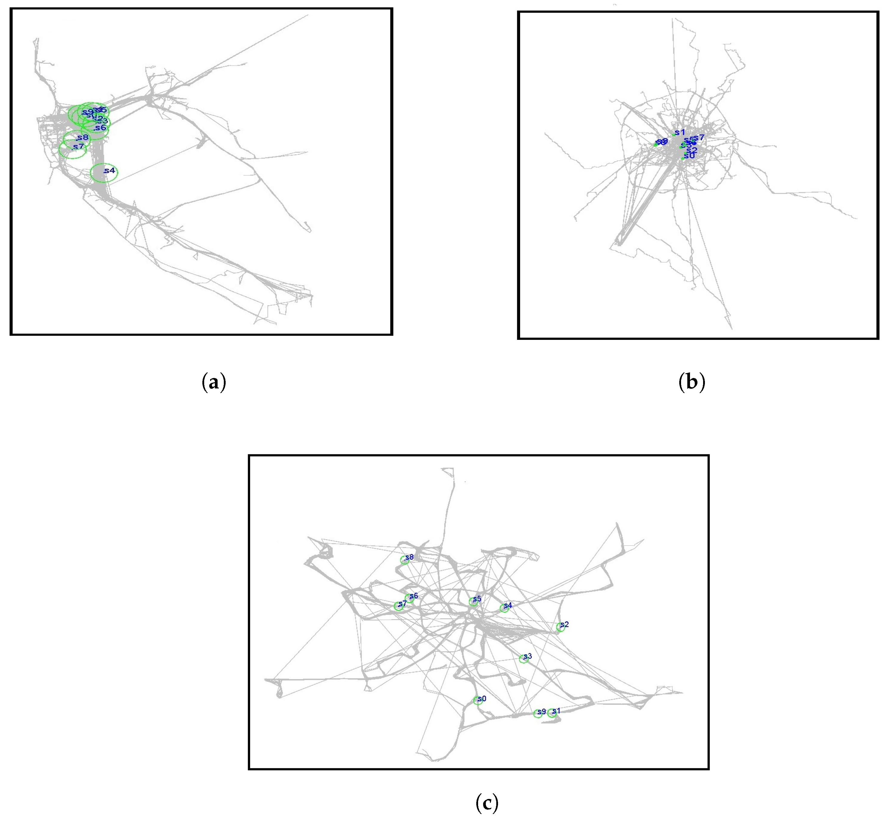
Providing a model requires data based on individual daily activity and movement, but such data are often unavailable in large sizes. During daily mobility, people make different decisions in various situations and may choose routes based on rush hour and traffic. This point is often missed in simulators. Therefore, for a solid overview, we used datasets with GPS coordinates of public transportation (bus) and taxis during routine daily work rather than the preset defaults in the simulator. We used three datasets, of which two are the mobility of taxis over some time based on passenger requests in the cities of San Francisco and Rome, and one is the mobility of buses in the city of Münster in Germany on a daily schedule. We chose these cities as they differ in urban structures (Figure 1). San Francisco is categorized as a modern urban structure with stylish and structured streets. Rome is a city with an old texture that has expanded irregularly. Münster is a town with an irregular street structure. We aimed to obtain the mobility of taxis and buses in San Francisco, Rome, and Münster, respectively. While taxis’ restrictions are less than those for buses, and some taxis drive on the streets without following all traffic regulations, buses in Münster have to follow specific routes, instructions, and driving regulations in the city. This reflects departing at a particular time from predetermined routes and stopping at specific points at a predefined time. With such structural differences in datasets, we expect changes in the mobility and density of the network nodes caused by the structure (city) and nature of the nodes (bus/taxi). We will describe the features and characteristics of each data set in the following subsections.

3.1.1. San Francisco Taxis

The first scenario is taxi mobility in San Francisco, USA [36]. This dataset contains GPS coordinates of 500 taxis during 30 days in the San Francisco Bay Area. The data were collected from Exploratorium—the science, art, and human perception museum, through the cab spotting project. Each taxi was equipped with a GPS receiver that sent the location of each taxi to a server. The time interval for sending data was less than 10 s (i.e., the status update of the taxi location). During the simulation studies, we used the GPS coordinates of 100 to 500 taxis and their timestamps for two days.

3.1.2. Rome Taxis

The second scenario is taxi mobility in Rome, Italy [37]. This dataset contains the GPS coordinates of 320 taxis during 30 days in Rome. This dataset was collected in February 2014. In the simulation studies, we used the GPS coordinate of 50 to 198 taxis and their timestamps for two days (1 February 2014 and 2 February 2014). We used the data of only 198 taxis because only 198 taxis were active within these two days.

3.1.3. Muenster Buses

To consider a scenario for public transportation, we created a novel dataset containing the route of buses following the schedule of public transportation in the city of Münster. We collected and converted data from Münster public utilities, live data website http://api.busradar.conterra.de/demo/. We collected the data on 4 July 2021 and 5 July 2021. There were 149 buses operating, but not all were active simultaneously. For example, only a limited number of buses were active at night.

3.2. Routing Algorithms

The most prevalent routing algorithms in OppNets are flooding-based, prediction-based, and history-based algorithms. Therefore, to measure and compare the performance of the networks under various conditions, we have used three routing algorithms of Epidemic, Prophet, and PPHB++ which are flooding, prediction, and history-based, respectively. In addition, PPHB++ is flexible in changing the number of message copies in the network. The performance is addressed in terms of Message Delivery Probability (MDP), Dropped Message Probability (DMP), and Network Overhead (NetO). In the following, we explain these algorithms briefly.
Epidemic algorithm: is the most straightforward algorithm in which messages are broadcast to all available neighbors [18]. This process is repeated until the message reaches the destination or expires (end of its Time To Live (TTL)). The network suffers a high overhead in this algorithm, and there is no optimal routing algorithm.
Prophet algorithm: is the most well known prediction-based algorithm [38]. The contact history of nodes is used to calculate MDP. Then, nodes with higher MDP carry the messages. When nodes are within the communication range of each other, they update their predictability list. Furthermore, nodes that are often in the communication range of each other will receive higher MDP.
PPHB++ algorithm: is based on Privacy-Preserving History-Based routing in the opportunistic networks (PPHB+) [39]. We have upgraded this algorithm to PPHB++ by restricting the Number of Message Copies (NumMC). In Prophet and Epidemic algorithms, when a node wants to send a message to a neighbor, it will send a message copy to the neighbor, and a copy remains in its buffer. While this is not the case in the PPHB++ algorithm, the nodes do not keep a copy for themselves.
Each node produces a polynomial in this algorithm, and the root of the polynomial is considered the node’s nickname. When a node constantly detects a neighbor in its communication range, it multiplies its polynomial to the neighbor’s polynomial and updates and delivers its new polynomial. When a node decides on carrying a message, it checks whether the message’s receiver nickname is the root of its polynomial. Suppose the message’s receiver nickname is the root of a node polynomial. In that case, it means that this node will most likely meet the receiver of the message, so it is a suitable candidate for carrying a message, and it can bring the message nearer to the destination.

3.3. Simulation Environment

We used the Opportunistic Network Environment (ONE) [40] to simulate and evaluate scenarios. Additionally, we used Matlab to calculate the outputs and depict the graphs and charts.
We imported the datasets into ONE. Each scenario continuance was 48 h, and the updating interval was 100 ms. Node mobility is according to the recorded GPS coordinate data in the datasets. The First-In, First-Out (FIFO) method is used for queuing models in buffers. The following parameters were configured and remained the same in all scenarios and simulations:
  • Message size: 500 k to 1 M;
  • Message Time To Live (TTL): 5 h;
  • Transmission interface: Bluetooth is the transmission interface in all simulations;
  • Transmission range: The maximum distance of forwarding a message from a node to a neighbor is 23 m. This range is based on experiments performed in [41].
We evaluated the performance of networks in the different scenarios, using the algorithms in terms of MDP, DMP, and NetO. We explicitly define these parameters in the ONE simulator as follows:
  • MDP: specifies the probability of delivering messages to the destination; Where:
    MDP = Delivered messages Created messages
  • DMP: specifies the probability of deleting messages in the nodes’ buffer due to the buffer saturation or TTL messages; Where:
    DMP = Dropped messages Started messages + Created messages
    Started messages are the number of message copies produced in the network. Nodes for forwarding a message to a neighbor in usual routing algorithms in ONE produce a copy of the message, forward it to the neighbor and retain a copy for themselves. Therefore, a considerable number of messages are started in the network.
  • NetO: is the ratio of passed relayed nodes subtracted by delivered messages to delivered messages; Where:
    NetO = Passed relayed nodes Delivered messages Delivered messages

3.4. Optimized Parameters

In order to investigate the network performance, we performed a two-phase study: (i) We considered the San Francisco dataset due to the nodes’ mobility and PPHB++ algorithm due to higher flexibility. We conducted the simulations to investigate the effect of different configurations of parameters on the network’s performance by calculating the optimized parameters for this particular dataset and algorithm. (ii) During the second phase, we used the optimized parameters obtained from the first phase to calculate the network performance under the other datasets and algorithms discussed earlier. We have identified the five most influential parameters on network performance: The Number of Message Copies (NumMC), Number of Nodes (NumN), Buffer Size (BuffS), Messages Interval (MI), and Node Mobility (NM). The first four parameters are configurable, while the fifth one is correlated with the structure of the dataset, collected data, and network topology. We configured these five parameters to observe their impact on the network performance (Table 1). Due to simulation restrictions, we considered four NumMC (1, 5, 10, and 50), three NumN (100, 250, and 500), three BuffS (5, 10, and 15), and three MI intervals with appropriate configurations (see Table 1). The rest of the states of these parameters were restricted to 50, 500, 15, and 25 to 35 for NumMC, NumN, BuffS, and MI, respectively. We used Machine Learning (ML) techniques, including decision tree, multiple linear, polynomial, random forest, and support vector regression (Reg), to predict the optimal outputs (Table 2). The Radial Basis Function (RBF) was used for the kernel of Support vector regression. We predict the optimized parameters for the extended versions of the configurations and network using ML. Furthermore, to mimic the real-world application and consider the restrictions, we have assumed that nodes in the network have limited resources, and the buffer size is 5 Mb.
While changing a parameter according to Table 1, the rest of the parameters remain constant and set as NumMC: 1, NumN: 100, BuffS: 5, MI: 25 to 30, Map: San Francisco, routing algorithm: PPHB++.
We evaluated the network’s performance using the regression score based on the coefficient of determination ( R 2 ). We only considered those with a score of above 0.9 for no less than three influencing terms of the performance. We used two different algorithms to predict the optimized parameters for each regression algorithm.
Algorithm 1: In each regression model, (i) the first row is the result ( R 1 = 1 ), (ii) in ith row of regression the following condition is checked: (iii) if the MDP i is greater than MDP in R 1 and DMP i is less than the DMP in R 1 , and the NetO i is less than the NetO in R 1 , (iv) the R 1 changes to i ( R 1 = i ).
Algorithm 1 Regression model
 Require:
R , i
 Ensure:
Alg1 result
    1:
Initialization:
    2:
Mechanism Initialization
    3:
Read the value R from row i
    4:
R 1 = 1
    5:
for i = 2 to the end of the array do
    6:
    if  M D P ( i ) > M D P ( R 1 ) and D M P ( i ) < D M P ( R 1 ) and N e t O ( i ) < N e t O ( R 1 )  then
    7:
         R 1 = i
    8:
    end if
    9:
end for
    10:
Alg1=NumMC( R 1 ),NumN( R 1 ),BuffS( R 1 ),MI( R 1 )
    11:
return  A l g 1
In Algorithm 2, with the inverse MDP, as well as with DMP and NetO as the influencing terms of network performance, the minimum X should be delivered in order to obtain the maximum performance. In this equation, we considered a = 100 , and b = 1 / 10 . Depending on the application and the aim of the study, the user can change the coefficients.
Algorithm 2 Regression model
 Input:
X , i
 Output:
Alg2 result
   1:
Initialization:
   2:
Mechanism Initialization
   3:
Read X from row i of the performance terms
   4:
X ( i ) = 1 M D P ( i ) + a D M P ( i ) + b N e t O ( i )          ▹ a and b are the coefficient
   5:
a = 100 a n d b = 1 10
   6:
R 2 =IndexMin (X)
   7:
Alg2=NumMC( R 2 ),N( R 2 ),B( R 2 ),MI( R 2 )
   8:
return A l g 2
Additionally, we considered the network with and without malicious nodes (Section 4.3.2). In order to compare the networks, we varied the NumN as: San Francisco: 100 to 500 nodes, Rome: 50 to 200 nodes, Münster: 50 to 150 nodes.
We set all networks based on the obtained optimized simulation results.

4. Results

4.1. Influencing Parameters and the Network Performance

Table 3 represents the effect of the aforementioned parameters on the network performance. We elaborate the impact of each parameter (NumMC, BuffS, MI, NumN, and NM) on network performance (MDP, DMP, NetO) as follows:

4.1.1. NumMC and Network Performance

Reducing the NumMC on the network has a limited and negligible effect on the MDP. The maximum value of MDP ( 75.59 % ) occurs when there is only one message on the network, and the minimum MDP value ( 72.03 % ) is delivered in the presence of ten message copies on the network. Although increasing the NumMC from one to ten causes a descending change in MDP, further increasing NumMC, does not necessarily follow this pattern. Removing the restrictions of NumMC delivers the NumMC value of 74.58 % . The difference between the Min and Max NumMC (i.e., 1 < NumMc < unlimited) is only 1 % .
Yet, NumMC causes a reduction in the DMP. The lowest value ( 1.13 % ) occurs when there are 50 messages on the network, and the highest value ( 2.23 % ) occurs when there are 10 message copies on the network. Although the DMP values are small, increasing the NumMC from 1 to 50 can reduce DMP up to 50 % of the primary value, which is significant. As the number of delivered messages increases, the number of messages dropped in the buffer decreases.
We expected increasing NumMC impacts NetO, inversely. The results show a significant increase in NetO with greater NumMC. The Min NetO ( 9.905 % ) is reached when NumMC is one, and the Max NetO is delivered ( 23.7 % ) when there are 50 message copies on the network. The results did not change much after increasing the messages to more than 50 (no limit to the number of messages).
In summary, although NumMC has a minor effect on MDP and DMP, it can significantly enhance NetO. Furthermore, when there are more than 50 messages (No limited), the result does not change in this routing algorithm.

4.1.2. BuffS and Network Performance

Increasing the BuffS from 5 to 15 and observing its impact on the network parameters delivers 1 % improvement in MDP, 16 % reduction in DMP, and NetO worsening by 0.64 % .
Therefore, BuffS does not significantly affect the MDP, DMP, and NetO. Increasing the buffer volume can reduce the number of dropped messages because messages are deleted either when the buffer is full or when it expires. Considering the network size, further increasing the BuffS beyond a certain point cannot significantly change the network’s performance (saturation).

4.1.3. MI and Network Performance

Increasing MI reduces the number of messages in the network. When the number of messages generated in the network decreases (greater MI), the messages are more likely to reach the destination. By changing MI from 5 to 15 to 25 to 35, MDP increases by 89 % . Moreover, the probability of deleting messages dropped by 40 % . Having more messages in the network leads to deleting them in the buffer earlier than sending them out to the other nodes. Increasing MI increases the NetO by 5 % .
Therefore, we can conclude that MI mainly affects MDP and DMP, while there is not much change in NetO.

4.1.4. NumN and Network Performance

As the number of nodes increases from 100 to 500, the MDP rate increases by 4 % , the DMP rate decreases by 46 % , and the NetO increases by 67 % as more nodes connect.
As expected, increasing the number of nodes in the network can outstandingly enhance DMP, have a negligible effect on MDP, and cause NetO to be worse.

4.1.5. NM and Network Performance

The last row of Table 3 displays the effect of NM on the network performance. In San Francisco, taxis have a wide range of mobility and travel in different directions. In Rome, taxis also have a wide range of mobility, but our data show a limited number of movements during the selected time.
In Münster, the range of buses is limited. They can only travel on restricted routes and stop at bus stops at specific times. Therefore, fewer nodes have the opportunity to meet each other and exchange data.
The MDP is higher because more nodes are connected in Table 3 in San Francisco. On the other hand, the amount of DMP in Rome and Münster is high due to the expiration of packets’ TTL and the saturation of the nodes’ buffer.
Regarding MDP and DMP, San Francisco has the best performance as a result of having many stimulus nodes, and Münster has the worst. The San Francisco network is better than Münster by around 9 times and 96 % in MDP and DMP, respectively. NetO in Münster is less than San Francisco 12 % due to fewer messages being exchanged in the network.
As a result, we can conclude that the node movement in the network can significantly impact MDP and DMP.
A closer look at Table 3 reveals that node mobility influences MDP and DMP changes. Considering the mobility of the nodes in the three datasets shows the noticeable changes under different conditions.
According to Equations (1) and (2), MDP and DMP are inversely related (not linear). Using the same analysis, the Münster dataset with the highest DMP and the San Francisco dataset with the lowest DMP behave as expected. NetO, unlike DMP and MDP, is influenced by several dominant parameters. NumMc, NumN, NM have the most significant impact on NetO, while BuffS and MI can be excluded from the factors affecting NetO. We can conclude that nodes and their related features, such as the number of messages of a node, the number of nodes, and the degree of mobility of the nodes, have the most significant impact on network performance. Similarly, in the real world, node types (taxis, buses, or pedestrians) and their characteristics (speed, route, and mobility) have the greatest influence on network performance.

4.2. Extending the Simulation Results Based on ML and Regression Models

Table 4 shows the results of the regression score based on the coefficient of determination ( R 2 ). Having scored one as the maximum, we omitted the Multiply linear regression from the list of qualifiers.

4.2.1. Obtaining the Optimized Influencing Parameters (OIP)

Comparing Table 4 and Table 5 indicates that the Decision Tree regression is the best performer. Comparing Algorithms 1 and 2 in the Decision Tree with a higher regression score delivers the optimized parameters: NumMC = 1, NumN = 100, BuffS = 10, MI = 15 to 25 s.

4.2.2. Obtaining the Optimized Influencing Parameters with Limited Resources (OIPL)

We summarize the optimal results according to Algorithms 1 and 2 for different regression algorithms in Table 6.
Similar to the previous subsection, we compared the different regression algorithms, but for the network with limited resources. Comparing Table 4 and Table 6 indicates Decision Tree regression as the best performer. Comparing the Algorithms 1 and 2 in Decision Tree with the higher regression score delivers the optimized parameters: NumMC = 1, NumN = 100, BuffS = 5, MI = 55 to 65 s.
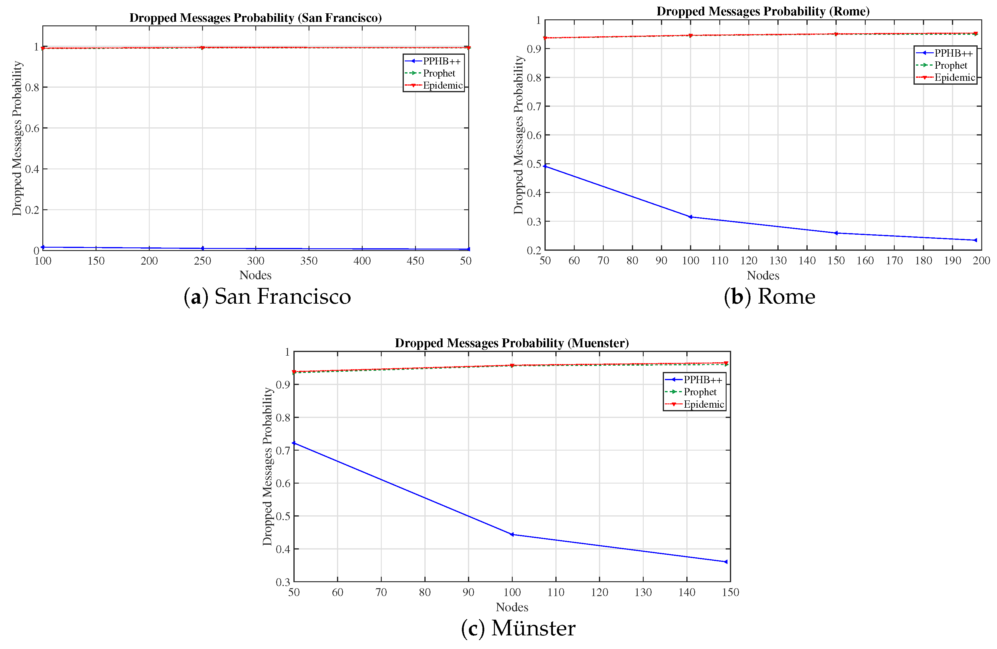
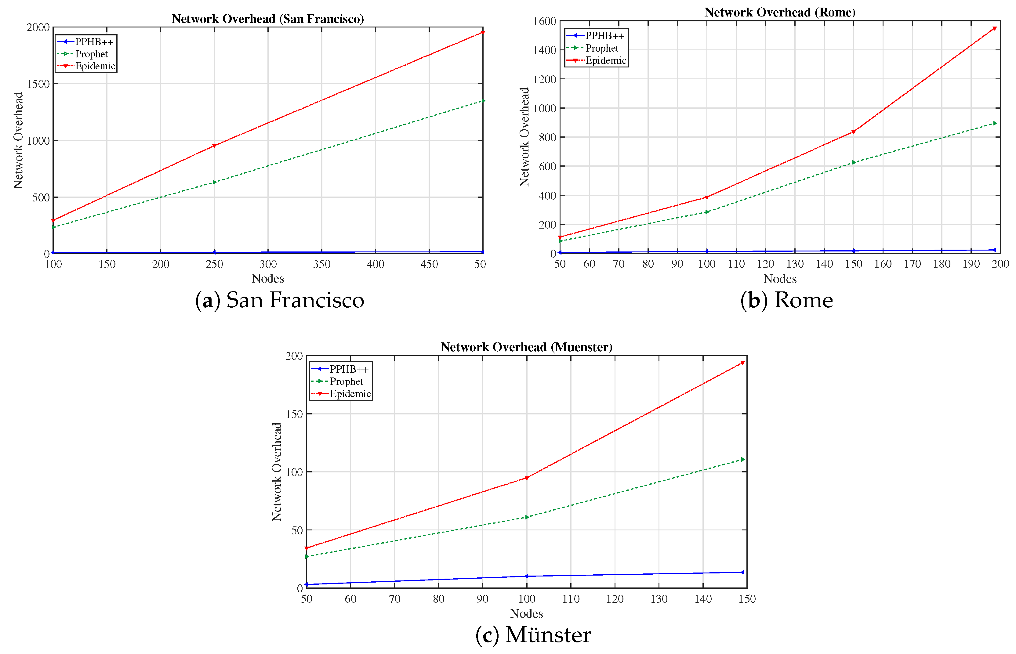
We have also simulated and calculated Decision Tree regression for Epidemic and Prophet algorithms based on these parameters. The results are illustrated in Figure 2. For PPHB++, Prophet, and Epidemic algorithms in Decision Tree regression, the average MDP is 80.2244 % , 25.1400 % , and 19.6533 % , respectively; the average DMP is 1.52 % , 99.9200 % , and 100.1644 % , respectively; and the average NetO is 12.8047 , 712.6886 , and 953.9167 , respectively. As the number of nodes increases, the number of messages in the network grows and, as a result, raises the network overhead in Prophet and Epidemic algorithms. The least overhead by PPHB++ is addressed by its fundamental difference with two other algorithms to avoid copying the message while forwarding it to a neighbor.

4.3. Network Performance

We evaluated the network performance for three concrete datasets by the optimized parameters obtained from the previous section. We also compared the network performance under three algorithms of PHHB++, Epidemic, and Prophet during the simulations.

4.3.1. Network Performance without the Malicious Nodes

Figure 3, Figure 4 and Figure 5 demonstrate the network’s performance without malicious nodes. We assumed all nodes were trusted and forwarded messages without any sabotage.
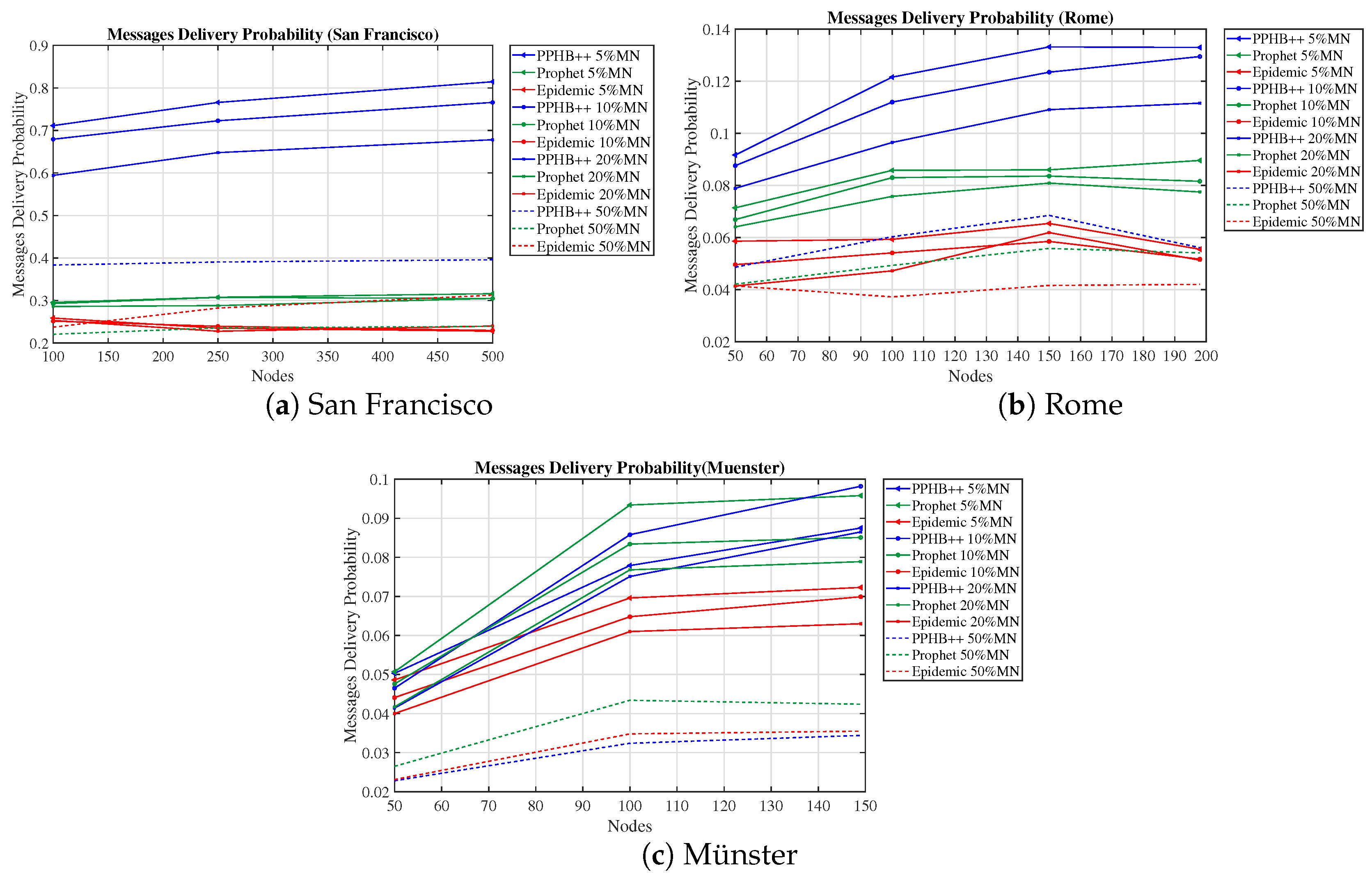
Figure 3 presents the MDP for all three datasets. The average MDP in different cities for PPHB++, Prophet, and Epidemic in San Francisco are 81 % , 31.17 % , and 23.70 % , respectively; in Rome, they are 9.9900 % , 8.6275 % , and 6.0975 % , respectively; in Münster, they are 7.19 % , 8 % , and 0.0635 % , respectively.
In San Francisco and Rome, the output patterns are relatively similar; the highest delivery is by the PPHB++ algorithm, followed by the Prophet and Epidemic. PPHB++ improved MDP compared to Prophet and Epidemic 159.9337 % and 241.9468 % , respectively, in San Francisco; and 15.7925 % and 63.8376 % respectively in Rome. The higher MDP of PPHB++ in San Francisco and Rome is due to the larger number and greater flexibility of taxis. This causes the chance of meeting two taxis to exchange a message to increase. Furthermore, in the Prophet algorithm, the messages are sent to the neighbors with higher MDP, but in the Epidemic algorithm, messages are broadcast blindly, which reduces MDP.
In Münster, the best MDP is delivered by the Prophet algorithm, then the PPHB++ and Epidemic algorithms. The Prophet algorithm yields a better result than PPHB++ ( 11.2193 % ) and Epidemic ( 25.9318 % ) in terms of MDP. Furthermore, Figure 3 supports the results in Table 3; in San Francisco, the MDP is between 23 % and 81 % due to a large number of active taxis with an extensive range of movement; in Rome, it is lower and between 6 % and 10 % because the number of active taxis and the mobility are smaller; in Münster, this value is between 7 % and 8 % because the type of node is changed to bus. Consequently, the number of buses is smaller than the other two previous scenarios, and their movement range in the city is limited.
A limited number of buses driving on particular routes following local public transportation regulations restricts mobility and flexibility. In contrast, the other two cities with taxis are more expansive in quantity, the radius of movement, and flexibility. As a result, messages have a better chance of reaching the destination directly or through intermediate nodes in San Francisco and Rome rather than Münster. Figure 4 represents the DMP for San Francisco, Rome, and Münster datasets. The average DMP in different cities for PPHB++, Prophet, and Epidemic are 1.15 % , 99.10 % , and 99.27 % , respectively, in San Francisco; they are 32.4975 % , 94.5500 % , and 94.7000 % , respectively, in Rome; and they are 50.8733 % , 95.0767 % , and 95.4100 % , respectively, in Münster.
The output patterns in all three cities are similar, with Epidemic and Prophet algorithms on top, giving the highest value of DMP, and PPHB++ with the least. Furthermore, Epidemic and Prophet behave the same way, giving an overlap output in Figure 4. Applying PPHB++ outperforms Prophet and Epidemic in DMP by 98.8396 % and 98.8416 % , respectively, in San Francisco; 65.6293 % and 65.6837 % , respectively, in Rome; and 46.4923 % and 46.6792 % , respectively, in Münster.
Under a high density of nodes, the PPHB++ algorithm delivers a better output, and with a low density of nodes, Prophet works better than the other two algorithms. The reason is the approach of forwarding the message from the source to a neighbor or destination in different algorithms. Having only one copy of a message in PPHB++ demands a higher density of the network, enabling message delivery. In contrast, in the Prophet algorithm, broadcasting the message to a neighbor or several is less restricted under certain conditions (higher probability of message delivery by a neighbor compared to the node itself). Therefore, MDP improves at the expense of NetO.
Figure 5 demonstrates the NetO for the San Francisco, Rome, and Münster datasets. The average NetO for PPHB++, Prophet, and Epidemic are 14.2523 , 738.2193 , and 1067.8 , respectively, in San Francisco; they are 14.4179 , 472.1325 , and 721.5618 , respectively, in Rome; and they are 8.9616 , 66.2785 , and 107.8029 , respectively, in Münster.
Epidemic in all three datasets has the highest NetO, while PPHP++ is at the bottom and Prophet is in between these two. The low DMP and NetO in the PPHB++ algorithm are due to minimal NumMC. Epidemic broadcasts the messages to all neighboring nodes and generates a copy message each iteration. This significantly increases the NetO by saturating the network and using the resources. Although in Prophet, the broadcasting is limited to specific nodes that satisfy the message probability requirements, the number of message copies is still noticeable. PPHB++ overcomes Prophet and Epidemic in NetO by 98.0694 % and 98.6653 % , respectively, in San Francisco; by 96.9462 % and 98.0018 % , respectively, in Rome; and by 86.4788 % and 91.6870 % , respectively, in Münster.

4.3.2. Network Performance with Malicious Nodes

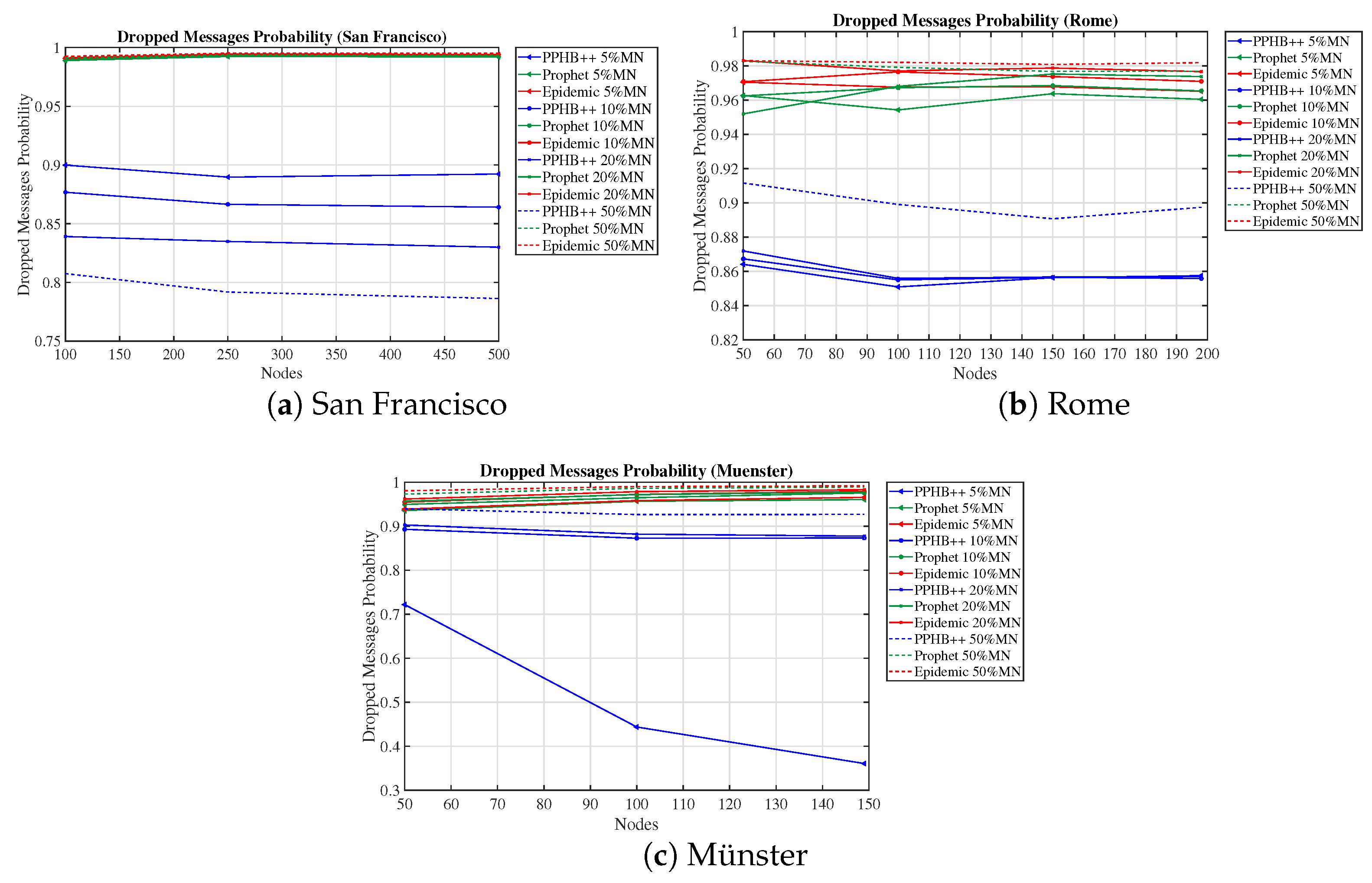
Figure 6, Figure 7 and Figure 8 present the network’s performance in the presence of the malicious nodes. We have considered the network with 5 % , 10 % , 20 % , and 50 % malicious nodes.
Figure 6 illustrates MDP for San Francisco, Rome, and Münster datasets. This figure confirms the results obtained from Figure 3. In San Francisco and Rome, the results are similar—the largest value is given by the PPHB++ algorithm, followed by the Prophet and Epidemic algorithms, respectively, for all cases with malicious nodes. In Münster, when 5 % of nodes are malicious, the best performance of MDP belongs to Prophet, PPHB++, and Epidemic algorithms, from top to bottom. When 10 % of nodes are malicious, this is rearranged to PPHB++, Prophet, and Epidemic algorithms. When the malicious nodes are 20 % , the best performance in MDP is for PPHB++, Prophet, and Epidemic algorithms, respectively. Finally, when 50 % of the nodes are malicious, Prophet, Epidemic, and PPHB++ algorithms work best, respectively.
When 10 % and 20 % of nodes are malicious, PPHB++ works more reliably than the other two. Whereas, in the case of 5 % and 50 % of nodes being malicious, the Prophet algorithm achieves a higher MDP.
Figure 7 shows DMP for San Francisco, Rome, and Münster datasets, and the results support Figure 4. PPHB++, Epidemic, and Prophet algorithms have the lowest DMP, respectively, in all scenarios.
Figure 8 displays the DMP for all three datasets. The lowest belongs to PPHB++, Prophet, and Epidemic algorithms in this figure. The reasons for these results are similar to what was mentioned in the previous section.

5. Discussion

5.1. Restrictions of the Study

We investigated the effect of NumMC, BuffS, MI, NumN, and NM as the influencing parameters on OppNets performance. We also evaluated the effect of the presence of malicious nodes on the network performance. Despite performing an extensive simulation study using three datasets, our work is limited in the number of datasets (restricted by node density and mobility), the number of nodes (maximum 500 nodes), and the amount of collected data (two days).

5.2. Influencing Parameters on the Network Performance

Our study shows that reducing NumMC has little effect on receiving or deleting messages, but it significantly reduces NetO. Compared to other algorithms, this reduction in the number of copies of messages has a notable impact on reducing DMP, NetO and increasing the MDP. Increasing node’s BuffS has little effect on MDP, DMP, and NetO.
Increasing the message generation interval, which produces fewer messages, can significantly reduce DMP, and increase MDP, but it has little effect on NetO.
Increasing the mobility of the nodes causes a notable increase in MDP and a significant reduction in DMP.
Increasing the network’s NumN causes more nodes’ interactions and enhances the MDP and DMP. It can also raise the NetO.
Therefore, as an output and application of our study in real world cases, we would suggest, for example, that in a VANET approach on a highway which is considered as a network with a low number of nodes and mobility where network overhead is not the case, and forwarding emergency and traffic messages has the priority, we should increase the message generation interval only to produce prioritized massages and increase the number of messages copy and buffer size in order to achieve the best network performance.
As the other scenario in real-world application, in which the network has a large number of nodes, low mobility, and a significant message generation, we can decrease the number of messages copied and prioritize the messages to increase message generation interval. Consequently, we can decrease the network overhead and improve message delivery in the network. An example of such a network might be an event such as a carnival in a city.

5.3. Machine Learning Techniques and Real Work Applications

By examining these parameters in various simulations and regression in ML (decision tree, multiple linear, polynomial, random forest, and support vector regressions), we found the optimized parameters for different networks. Utilizing three networks with different features represented by three datasets in the real world shows that the optimal results are obtained when NumMC is one, the NumN is 100, the BuffS is 10, and MI is 15 to 25 s. Since the buffer is one of the limited resources in each node and is considered a severe restriction in real-world applications, we also calculated the best result when the BuffS is 5. The optimized parameters under this conditions are obtained as BuffS = 5, the NumMC = 1, the number of nodes in the network = 100, and the MI = 55 to 65 s. We used these parameters to set the network. However, to improve the accuracy and efficiency of using the lower volume of memory, in particular, for the big data including a large number of inputs (i.e., if the number of datasets is significantly increased), where the training and testing speed and time, computational resources, classification, and prediction are crucial, the neural-like structure of non-iterative models such as the successive geometric transformations model (SGTM) can be used. These methods usually provide a lower error value for the regression task. Ito decomposition (Kolmogorov–Gabor polynomial) can be used in combination with SGTM to extend the inputs of the SGTM [42].
We evaluated the network performance in terms of MDP, DMP, NumN, NM, and NetO on three concrete datasets with PPHB++, Prophet, and Epidemic routing algorithms. The results show that PPHB++ has better MDP in San Francisco and Rome because of their free movement, and Prophet delivers a better MDP in the Münster dataset. PPHB++ is the best performer in terms of DMP and NetO, followed by the Prophet and Epidemic algorithms.
We also estimated the impact of malicious nodes on network performance. We studied three algorithms with the presence of different numbers of malicious nodes. Algorithm PPHB++ has the best performance in MDP, DMP, and NetO with malicious network nodes without restricting the nodes’ movement. When there are constraints on node paths, the Prophet algorithm only works better in MDP.
In the San Francisco scenarios, where there are more nodes in the network, they acted slightly differently in the presence of malicious nodes.
According to the results, each network parameter can be set efficiently to have the best performance according to the network’s conditions and needs and consider what percentage of network nodes may be malicious. Our comprehensive study shows that network performance influences parameters configured based on the applications and restrictions. Depending on the importance of the terms of performance in each application, the influencing parameters might be weighted to deliver the output. Using ML techniques for considering network behavior under various features, influencing parameters, and datasets representing a real-world application allowed us to extend the study by predicting different scenarios in a network significantly.

5.4. Comparison of ONE Default Setting with Optimized Parameters

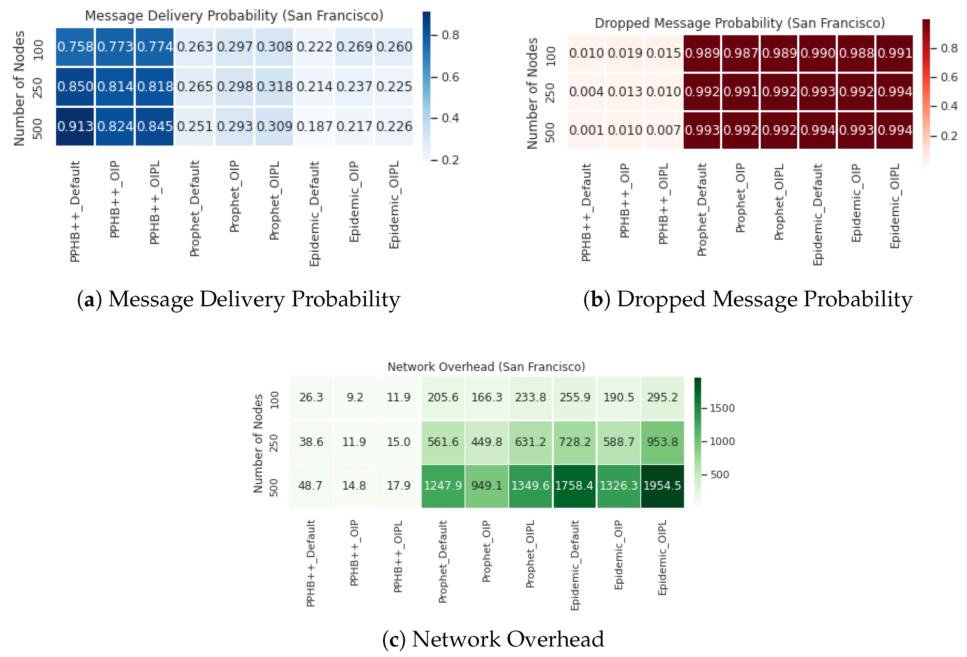
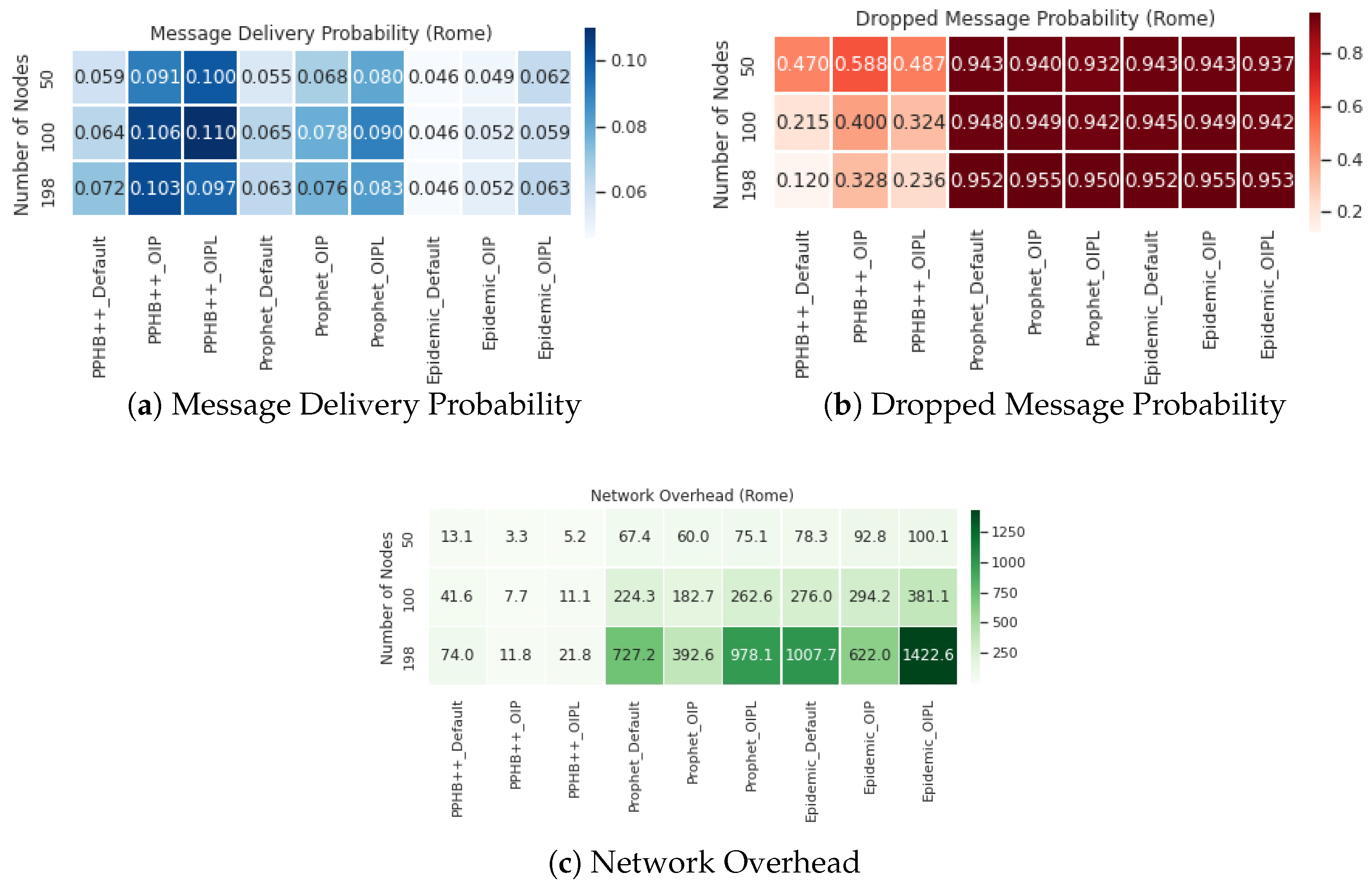
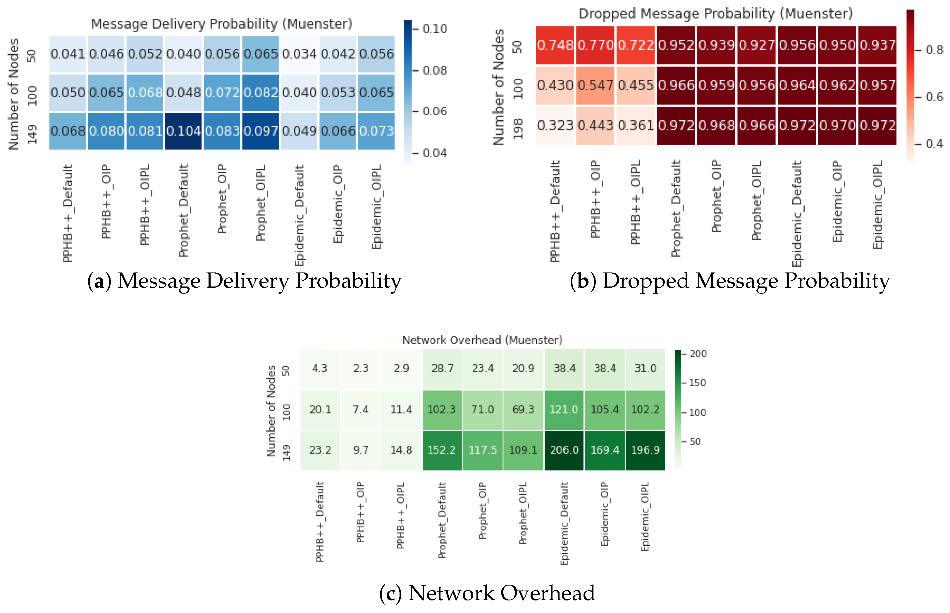
Figure 9, Figure 10 and Figure 11 present the results of ONE default setting, Optimized Influence Parameter (OIP), and Optimized Influencing Parameters with Limited resources (OIPL) under the specified conditions stated earlier. More details regarding these results are provided in Appendix A. Furthermore, we have compared OIP and OIPL results with the default setting to calculate the network performance’s enhancement (if any). We performed this experiment and compared all influencing parameters for the San Francisco, Rome, and Münster datasets. Thus, the results are represented as Improved OIP Improved OIPL for MDP, DMP, NetO.
For the Prophet algorithm, MDP increased by an average of 17 % in San Francisco and 32 % in the Rome and Münster datasets. For the Epidemic algorithm, increasing the number of nodes in all conditions reduces the MDP at different rates; however, in general, MDP increased by an average of 15 % in San Francisco and 34 % in the Rome and Münster dataset. OIP and OIPL are significantly positive in average improvement in all datasets under the Epidemic algorithm. Although OIP for 250 nodes in San Francisco delivers the lowest MDP, no meaningful pattern is observed.
The impact of DMP for OIP and OIPL is negligible in the Prophet and Epidemic algorithms in all datasets. This effect under PPHB++ has quite the inverse negative impact on San Francisco and Rome, and it is, on average, an increase of 20 % in the Münster dataset.
The results indicate an improvement of NetO in all datasets and algorithms; however, the improvement in the PPHB++ algorithm is greater (for example, 84 % in the Rome dataset). Under PPHB++, NetO decreased by an average of 18 % for OIP, but it also experienced an average of 15 % for OIPL in San Francisco. It presents an average of 60 % decrease in the San Francisco dataset. For the Prophet algorithm, NetO decreased by an average of 25 % for OIP, but increased by an average of 21 % for OIPL in Rome. NetO decreased by an average of 4 % for OIP, but increased by an average of 36 % for OIPL in Rome for the Epidemic algorithm. NetO is decreased by an average of 19 % for Prophet and Epidemic algorithms in the Münster dataset. Analyzing the results shows that the presented solution influences MDP and NetO significantly in all three datasets and algorithms (there are some exceptions) and remains neutral for DMP.

6. Conclusions

In real-world applications, wearable devices, taxis, and buses might be the nodes of opportunistic networks to save-carry-forward a message from the source to the destination, particularly when facing a lack of infrastructure or sending an emergency alert from an injured involved in an accident to a hospital or rescue team. Albeit with various weights, NumMC, BuffS, MI, NumN, and NM influence the network’s performance. To explore the real-world applications’ restrictions and impact of resources on the network performance, we deployed three datasets that differed in features and structures to represent the characteristics of such networks. Extensive simulations and analyses are required to show the impact of each factor on the network’s performance. We found that the nodes and the respective features are the most significant influences on the network performance represented by MDP, DMP, and NetO. This means that NumN, NM, and NumMC have greater weights than BuffS and MI. In the real world, this is mapped to the type of node (taxi or bus), its speed (NM), and the route it follows. All these factors are impacted by the route and regulation features determined by the dataset represented by the algorithm used in the simulation.
In a vast network, this requires specific configuration and tests. Thus, we used regressions techniques of machine learning to predict the optimized parameters for both networks with(out) resource restrictions.
We showed that obtaining the optimized parameters in each scenario rather than general configuration improves the network performance under different routine algorithms (i.e., PPHB++, Prophet, and Epidemic). Applying the optimized parameters to the network, MDP improved by an average of 17 % in San Francisco and 32 % in Rome and Münster (Prophet algorithm). In the same manner, MDP was enhanced by an average of 15 % in San Francisco and 34 % in Rome and Münster (Epidemic algorithm). In all datasets, the impact of DMP is negligible for the Prophet and Epidemic algorithms. Still, it has an inverse negative impact on PPHB++ in San Francisco and Rome and increases by 20 % in the Münster dataset. NetO was improved across all datasets and algorithms, although the PPHB++ algorithm gained the most.
A dense network may improve the probability of delivering a message, but increase the NetO. We concluded that public transportation could be used in OppNets depending on the purpose of the application. However, care must be taken to choose the appropriate means (wearables/taxis/bus) depending on the purpose and structure of the environment (city). Our study showed that buses with lower NetO are appropriate in OppNets if the message is time-tolerant.
The results indicated that using taxis in modern texture cities with a higher network overhead (e.g., several taxis in the same area and direction), greater speed (NM), and fewer restrictions on driving are suitable.
The datasets’ features restrict our work in terms of data acquisition (two days) and node characterizations (limited by node density and mobility and 500 nodes). For future work, we plan to consider pedestrians included in our dataset. Therefore, we plan to implement an OppNet on several wearable devices deployed in real situations with true-to-life scenarios. In addition, we would like to compare these results with the simulation outcomes and improve the ML algorithms in terms of performance, speed, and time to train.
Author Contributions

Conceptualization, S.R.; methodology, S.R. and T.H.; software, S.R.; validation, S.R. and T.H.; formal analysis, S.R. and T.H.; investigation, S.R.; resources, S.R.; data curation, S.R.; writing—original draft preparation, S.R. and T.H.; writing—review and editing, S.R. and T.H.; visualization, S.R.; supervision, T.H.; project administration, T.H.; funding acquisition, T.H. All authors have read and agreed to the published version of the manuscript.

Funding

We acknowledge support from the Open Access Publishing Fund of University of Muenster.

Institutional Review Board Statement

Not applicable.

Informed Consent Statement

Not applicable.

Data Availability Statement

Not applicable.

Acknowledgments

We acknowledge support from the Open Access Publishing Fund of University of Muenster.

Conflicts of Interest

The authors declare no conflict of interest.

Abbreviations

The following abbreviations are used in this manuscript:
OppNetOpportunistic Networks
MLMachine Learning
RegRegression
MDPMessage Delivery Probability
DMPDropped Message Probability
NetONetwork Overhead
ONEOpportunistic Network Environment
FIFOFirst In First Out
TTLTime To Live
NumMCNumber of Messages Copies
NumNNumber of Nodes
BuffSBuffer Size
MIMessages Interval
NMNode Mobility
OIPOptimized Influencing Parameters
OIPLOptimized Influencing Parameters with Limited resources

Appendix A

The detail of the results illustrated in Figure 9, Figure 10 and Figure 11 are provided in Table A1, Table A2 and Table A3, respectively, in the followings. The MDP and DMP parameters are normalized in these tables between 0 and 1.
Table A1. Comparison of ONE default setting with Optimized parameters for San Francisco dataset.
NumNRouting alg.ParametersMDPDMPNetO
100PPHB++Default 0.7577 0.0099 26.2536
OIP 0.7731 0.0193 9.2411
Improved OIP 2 % 95 % 65 %
OIPL 0.7740 0.0153 11.8901
Improved OIPL 2 % 55 % 55 %
ProphetDefault 0.2631 0.9891 205.5978
OIP 0.2970 0.9868 166.3056
Improved OIP 13 % 0.23 % 19 %
OIPL 0.3080 0.9888 233.8289
Improved OIPL 17 % 0.03 % 14 %
EpidemicDefault 0.2221 0.9903 255.9415
OIP 0.2685 0.9878 190.4832
Improved OIP 21 % 0.25 % 26 %
OIPL 0.2601 0.9907 295.1669
Improved OIPL 17 % 0.04 % 15 %
250PPHB++Default 0.8497 0.0038 38.5818
OIP 0.8144 0.0126 11.8671
Improved OIP 4 % 231 % 69 %
OIPL 0.8182 0.0098 14.9696
Improved OIPL 4 % 157 % 61 %
ProphetDefault 0.2647 0.9922 561.5886
OIP 0.2984 0.9907 449.7669
Improved OIP 13 % 0.15 % 20 %
OIPL 0.3177 0.9921 631.2182
Improved OIPL 20 % 0.01 % 12 %
EpidemicDefault 0.2142 0.9933 728.2462
OIP 0.2369 0.9919 588.7030
Improved OIP 11 % 0.16 % 19 %
OIPL 0.2246 0.9939 953.7604
Improved OIPL 5 % 0.06 % 30 %
500PPHB++Default 0.9135 0.0014 48.7044
OIP 0.8236 0.0100 14.7644
Improved OIP 10 % 614 % 70 %
OIPL 0.8451 0.0068 17.8872
Improved OIPL 7 % 385 % 63 %
ProphetDefault 0.2514 0.9933 1247.9009
OIP 0.2928 0.9916 949.0570
Improved OIP 16 % 0.17 % 24 %
OIPL 0.3095 0.9922 1349.6107
Improved OIPL 23 % 0.11 % 8 %
EpidemicDefault 0.1866 0.9943 1758.3541
OIP 0.2170 0.9926 1326.3259
Improved OIP 16 % 0.17 % 0.24 %
OIPL 0.2262 0.9936 1954.4749
Improved OIPL 21 % 0.07 % 11 %
Table A2. Comparison of ONE default setting with optimized parameters for Rome dataset.
NumNRouting alg.ParametersMDPDMPNetO
50PPHB++Default 0.0591 0.4697 13.0696
OIP 0.0911 0.5879 3.3213
Improved OIP 54 % 25 % 75 %
OIPL 0.1000 0.4866 5.2172
Improved OIPL 15 % 4 % 60 %
ProphetDefault 0.0553 0.9428 67.4149
OIP 0.0677 0.9401 60.0234
Improved OIP 22 % 0.28 % 11 %
OIPL 0.0804 0.9323 75.1202
Improved OIPL 45 % 1 % 11 %
EpidemicDefault 0.0459 0.9425 78.2687
OIP 0.0485 0.9432 92.7646
Improved OIP 6 % 0.07 % 19 %
OIPL 0.0624 0.9367 100.0608
Improved OIPL 36 % 0.61 % 28 %
100PPHB++Default 0.0643 0.2148 41.5878
OIP 0.1056 0.3997 7.6695
Improved OIP 64 % 86 % 82 %
OIPL 0.1099 0.3236 11.1034
Improved OIPL 71 % 51 % 73 %
ProphetDefault 0.0648 0.9476 224.3087
OIP 0.0780 0.9485 182.6512
Improved OIP 20 % 0.09 % 19 %
OIPL 0.0903 0.9417 262.5534
Improved OIPL 39 % 0.62 % 17 %
EpidemicDefault 0.0460 0.9446 276.0037
OIP 0.0523 0.9490 294.1793
Improved OIP 14 % 0.46 % 7 %
OIPL 0.0589 0.9422 381.0702
Improved OIPL 28 % 0.25 % 38 %
198PPHB++Default 0.0719 0.1203 74.0166
OIP 0.1032 0.3281 11.7825
Improved OIP 44 % 173 % 84 %
OIPL 0.0968 0.2358 21.8399
Improved OIPL 35 % 96 % 70 %
ProphetDefault 0.0633 0.9524 727.1995
OIP 0.0762 0.9554 392.5911
Improved OIP 20 % 0.31 % 46 %
OIPL 0.0830 0.9499 978.1411
Improved OIPL 31 % 0.26 % 34 %
EpidemicDefault 0.0463 0.9516 1007.6753
OIP 0.0519 0.9547 621.9957
Improved OIP 12 % 0.32 % 38 %
OIPL 0.0634 0.9527 1422.5815
Improved OIPL 37 % 0.11 % 41 %
Table A3. Comparison of ONE default setting with optimized parameters for Münster dataset.
NumNRouting alg.ParametersMDPDMPNetO
50PPHB++Default 0.0413 0.7478 4.3154
OIP 0.0459 0.7696 2.2808
Improved OIP 11 % 3 % 47 %
OIPL 0.0517 0.7222 2.9400
Improved OIPL 25 % 3 % 32 %
ProphetDefault 0.0397 0.9520 28.7069
OIP 0.0555 0.9389 23.3992
Improved OIP 40 % 1 % 18 %
OIPL 0.0648 0.9267 20.9415
Improved OIPL 63 % 3 % 27 %
EpidemicDefault 0.0337 0.9562 38.4416
OIP 0.0418 0.9500 38.3757
Improved OIP 24 % 0.64 % 0.17 %
OIPL 0.0555 0.9371 30.9627
Improved OIPL 65 % 2 % 19 %
100PPHB++Default 0.0499 0.4296 20.1438
OIP 0.0645 0.5474 7.4186
Improved OIP 29 % 27 % 63 %
OIPL 0.0682 0.4551 11.3838
Improved OIPL 37 % 6 % 43 %
ProphetDefault 0.0475 0.9658 102.2734
OIP 0.0725 0.9588 70.9595
Improved OIP 53 % 0.72 % 31 %
OIPL 0.0820 0.9558 69.2689
Improved OIPL 73 % 1 % 32 %
EpidemicDefault 0.0395 0.9642 121.0390
OIP 0.0529 0.9618 105.3774
Improved OIP 34 % 0.02 % 13 %
OIPL 0.0651 0.9572 102.2169
Improved OIPL 65 % 0.72 % 16 %
149PPHB++Default 0.0676 0.3226 23.2323
OIP 0.0802 0.4431 9.7300
Improved OIP 19 % 37 % 58 %
OIPL 0.0805 0.3613 14.8462
Improved OIPL 19 % 12 % 36 %
ProphetDefault 0.1043 0.9718 152.1774
OIP 0.0825 0.9676 117.5335
Improved OIP 21 % 0.43 % 23 %
OIPL 0.0974 0.9656 109.0989
Improved OIPL 7 % 0.63 % 28 %
EpidemicDefault 0.0488 0.9724 205.9755
OIP 0.0664 0.9695 169.3973
Improved OIP 36 % 0.29 % 18 %
OIPL 0.0726 0.9724 196.8863
Improved OIPL 49 % 0 % 4 %

References

  1. Pozza, R.; Nati, M.; Georgoulas, S.; Moessner, K.; Gluhak, A. Neighbor discovery for opportunistic networking in internet of things scenarios: A survey. IEEE Access 2015, 3, 1101–1131. [Google Scholar] [CrossRef]
  2. Haghi, M.; Neubert, S.; Geissler, A.; Fleischer, H.; Stoll, N.; Stoll, R.; Thurow, K. A flexible and pervasive IoT-based healthcare platform for physiological and environmental parameters monitoring. IEEE Internet Things J. 2020, 7, 5628–5647. [Google Scholar] [CrossRef]
  3. Orlowski, A.; Romanowska, P. Smart Cities Concept: Smart Mobility Indicator. Cybern. Syst. 2019, 50, 118–131. [Google Scholar] [CrossRef]
  4. Haghi, M.; Danyali, S.; Ayasseh, S.; Wang, J.; Aazami, R.; Deserno, T.M. Wearable devices in health monitoring from the environmental towards multiple domains: A survey. Sensors 2021, 21, 2130. [Google Scholar] [CrossRef]
  5. Sestino, A.; Prete, M.I.; Piper, L.; Guido, G. Internet of Things and Big Data as enablers for business digitalization strategies. Technovation 2020, 28, 102173. [Google Scholar] [CrossRef]
  6. Martín-Campillo, A.; Crowcroft, J.; Yoneki, E.; Martí, R. Evaluating opportunistic networks in disaster scenarios. J. Netw. Comput. Appl. 2013, 36, 870–880. [Google Scholar] [CrossRef]
  7. Cuka, M.; Elmazi, D.; Bylykbashi, K.; Spaho, E.; Ikeda, M.; Barolli, L. Implementation and performance evaluation of two fuzzy-based systems for selection of IoT devices in opportunistic networks. J. Ambient. Intell. Humaniz. Comput. 2019, 10, 519–529. [Google Scholar] [CrossRef]
  8. Conti, M.; Giordano, S.; May, M.; Passarella, A. From opportunistic networks to opportunistic computing. IEEE Commun. Mag. 2010, 48, 126–139. [Google Scholar] [CrossRef]
  9. Boldrini, C.; Lee, K.; Önen, M.; Ott, J.; Pagani, E. Opportunistic networks. Comput. Commun. 2014, 48, 1–4. [Google Scholar] [CrossRef]
  10. Aguilar, S.; Vidal, R.; Gomez, C. Opportunistic sensor data collection with bluetooth low energy. Sensors 2017, 17, 159. [Google Scholar] [CrossRef]
  11. Aloi, G.; Caliciuri, G.; Fortino, G.; Gravina, R.; Pace, P.; Russo, W.; Savaglio, C. Enabling IoT interoperability through opportunistic smartphone-based mobile gateways. J. Netw. Comput. Appl. 2017, 81, 74–84. [Google Scholar] [CrossRef]
  12. Pelusi, L.; Passarella, A.; Conti, M. Opportunistic networking: Data forwarding in disconnected mobile ad hoc networks. IEEE Commun. Mag. 2006, 44, 134–141. [Google Scholar] [CrossRef]
  13. Ferretti, S. Shaping opportunistic networks. Comput. Commun. 2013, 36, 481–503. [Google Scholar] [CrossRef]
  14. Huang, C.M.; Lan, K.C.; Tsai, C.Z. A survey of opportunistic networks. In Proceedings of the 22nd International Conference on Advanced Information Networking and Applications-Workshops (Aina Workshops 2008), Gino-wan, Japan, 25–28 March 2008; pp. 1672–1677. [Google Scholar]
  15. Ali, A.H.K.; Lenando, H.; Chaoui, S.; Alrfaay, M.; Tawfeek, M.A. A Dynamic Resource-Aware Routing Protocol in Resource-Constrained Opportunistic Networks. CMC Comput. Mater. Contin. 2022, 70, 4147–4167. [Google Scholar]
  16. Khalil, A.; Abou Haidar, N.; Bassil, G.; Chbeir, R. Adaptive Resource Management Solution for Ad-Hoc Opportunistic Networks. Wirel. Pers. Commun. 2021, 117, 1931–1958. [Google Scholar] [CrossRef]
  17. Garg, K.; Giordano, S.; Förster, A. A study to understand the impact of node density on data dissemination time in opportunistic networks. In Proceedings of the 2nd ACM Workshop on High Performance Mobile Opportunistic Systems, Barcelona Spain, 3–8 November 2013; pp. 9–16. [Google Scholar]
  18. Vahdat, A.; Becker, D. Epidemic routing for partially connected ad hoc networks. Tech. Rep. CS-200006 2000. [Google Scholar] [CrossRef]
  19. Jesús-Azabal, M.; Herrera, J.L.; Laso, S.; Galán-Jiménez, J. OPPNets and Rural Areas: An Opportunistic Solution for Remote Communications. Wirel. Commun. Mob. Comput. 2021, 1–11. [Google Scholar] [CrossRef]
  20. Kuppusamy, V. Performance analysis of epidemic routing in destination-less oppnets. In Proceedings of the 2018 IEEE 19th International Symposium on “A World of Wireless, Mobile and Multimedia Networks” (WoWMoM), Chania, Greece, 12–15 June 2018; pp. 1–3. [Google Scholar]
  21. Candra, R.A.; Ilham, D.N.; Suherman, S.; Sani, A.; Tarigan, D. The Impact of Buffer Queue Interface Size to The 802.11 Ad Hoc Network Performances. In Proceedings of the IOP Conference Series: Materials Science and Engineering; IOP Publishing: Bristol, UK, 2019; Volume 506, p. 012039. [Google Scholar]
  22. Shen, J.; Moh, S.; Chung, I.; Sun, X. Buffer scheme optimization of epidemic routing in delay tolerant networks. J. Commun. Netw. 2014, 16, 656–666. [Google Scholar] [CrossRef]
  23. Kang, M.W.; Seo, D.Y.; Chung, Y.W. An efficient delay tolerant networks routing protocol for information-centric networking. Electronics 2020, 9, 839. [Google Scholar] [CrossRef]
  24. Socievole, A.; Caputo, A.; De Rango, F.; Fazio, P. Routing in mobile opportunistic social networks with selfish nodes. Wirel. Commun. Mob. Comput. 2019, 2019, 1–15. [Google Scholar] [CrossRef]
  25. Ciobanu, R.I.; Dobre, C.; Dascalu, M.; Trausan-Matu, S.; Cristea, V. Collaborative selfish node detection with an incentive mechanism for opportunistic networks. In Proceedings of the 2013 IFIP/IEEE International Symposium on Integrated Network Management (IM 2013), Ghent, Belgium, 27–31 May 2013; pp. 1161–1166. [Google Scholar]
  26. Hossen, M.S. DTN routing protocols on two distinct geographical regions in an opportunistic network: An analysis. Wirel. Pers. Commun. 2019, 108, 839–851. [Google Scholar] [CrossRef]
  27. Xiao, Y.; Wu, J. Data transmission and management based on node communication in opportunistic social networks. Symmetry 2020, 12, 1288. [Google Scholar] [CrossRef]
  28. Huang, C.; Jiang, P. Message Cache Management Optimization Research for Community-based Opportunistic Network. In Proceedings of the 3rd International Conference on Computer Engineering, Information Science & Application Technology, Chongqing, China, 30–31 May 2019. [Google Scholar]
  29. Soares, V.N.; Farahmand, F.; Rodrigues, J.J. Evaluating the impact of storage capacity constraints on vehicular delay-tolerant networks. In Proceedings of the 2009 Second International Conference on Communication Theory, Reliability, and Quality of Service, Colmar, France, 20–25 July 2009; pp. 75–80. [Google Scholar]
  30. Goudar, G.; Batabyal, S. Optimizing bulk transfer size and scheduling for efficient buffer management in mobile opportunistic networks. IEEE Trans. Mob. Comput. 2021, 1–16. [Google Scholar] [CrossRef]
  31. Bylykbashi, K.; Spaho, E.; Barolli, L.; Xhafa, F. Impact of node density and TTL in vehicular delay tolerant networks: Performance comparison of different routing protocols. Int. J. Space-Based Situated Comput. 2017, 7, 136–144. [Google Scholar] [CrossRef]
  32. Garg, P.; Dixit, A.; Sethi, P.; Pinheiro, P.R. Impact of Node Density on the QoS Parameters of Routing Protocols in Opportunistic Networks for Smart Spaces. Mob. Inf. Syst. 2020, 1–18. [Google Scholar] [CrossRef]
  33. Ge, L.; Jiang, S. An Efficient Routing Scheme Based on Node Attributes for Opportunistic Networks in Oceans. Entropy 2022, 24, 607. [Google Scholar] [CrossRef]
  34. Herrera-Tapia, J.; Förster, A.; Hernández-Orallo, E.; Udugama, A.; Tomas, A.; Manzoni, P. Mobility as the main enabler of opportunistic data dissemination in urban scenarios. In Proceedings of the International Conference on Ad-Hoc Networks and Wireless; Springer: Cham, Switzerlands, 2017; pp. 107–120. [Google Scholar]
  35. Kandhoul, N.; Dhurandher, S.K. An efficient and secure data forwarding mechanism for opportunistic IoT. Wirel. Pers. Commun. 2021, 118, 217–237. [Google Scholar] [CrossRef]
  36. Piorkowski, M.; Sarafijanovic-Djuki, N.; Grossglauser, M. A Parsimonious Model of Mobile Partitioned Networks with Clustering. In Proceedings of the First International Conference on COMmunication Systems and NETworkS (COMSNETS), Bangalore, India, 5–10 January 2009. [Google Scholar] [CrossRef]
  37. Bracciale, L.; Bonola, M.; Loreti, P.; Bianchi, G.; Amici, R.; Rabuffi, A. CRAWDAD Dataset Roma/Taxi (v. 2014-07-17). 2014. Available online: https://crawdad.org/roma/taxi/20140717/ (accessed on 5 August 2022).
  38. Lindgren, A.; Doria, A.; Schelén, O. Poster: Probabilistic routing in intermittently connected networks. In Proceedings of the Fourth ACM International Symposium on Mobile Ad Hoc Networking and Computing, Annapolis, MD, USA, 1–3 June 2003; pp. 90–100. [Google Scholar]
  39. Rashidibajgan, S.; Hupperich, T.; Doss, R.; Förster, A. Secure and privacy-preserving structure in opportunistic networks. Comput. Secur. 2021, 104, 102208. [Google Scholar] [CrossRef]
  40. Keränen, A.; Ott, J.; Kärkkäinen, T. The ONE simulator for DTN protocol evaluation. In Proceedings of the 2nd International Conference on Simulation Tools and Techniques, Rome, Italy, 2–6 March 2009; p. 55. [Google Scholar]
  41. Rashidibajgan, S.; Hupperich, T.; Doss, R.; Pan, L. Opportunistic Tracking in Cyber-Physical Systems. In Proceedings of the 19th International Conference on Trust, Security and Privacy in Computing and Communications (TrustCom), Guangzhou, China, 29 December–1 January 2020; pp. 1672–1679. [Google Scholar]
  42. Tkachenko, R.; Izonin, I.; Vitynskyi, P.; Lotoshynska, N.; Pavlyuk, O. Development of the Non-Iterative Supervised Learning Predictor Based on the Ito Decomposition and SGTM Neural-Like Structure for Managing Medical Insurance Costs. Data 2018, 3, 46. [Google Scholar] [CrossRef] [Green Version]
Figure 1. The structure of the city of (a) San Francisco (b) Rome (c) Muenster.
Jsan 11 00061 g001
Figure 2. Decision Tree regression for PPHB++, Epidemic, and Prophet algorithms. (a) Messages Delivery Probability (MDP). (The y-axis parameter is normalized to a scale between 0 and 1). (b) Dropped Messages Probability (DMP). (The y-axis parameter is normalized to a scale between 0 and 1). (c) Network Overhead.
Jsan 11 00061 g002
Figure 3. Messages delivery probability (MDP) for the three cities of San Francisco, Rome, and Münster (The y-axis parameter is normalized to a scale between 0 and 1).
Jsan 11 00061 g003
Figure 4. Dropped message probability (DMP) for the three cities of San Francisco, Rome, and Münster (The y-axis parameter is normalized to a scale between 0 and 1).
Jsan 11 00061 g004
Figure 5. Network overhead (NetO) for the three cities of San Francisco, Rome, and Münster.
Jsan 11 00061 g005
Figure 6. Message delivery probability (MDP) for the three cities of San Francisco, Rome, and Münster with the presence of malicious nodes in the network (the y-axis parameter is normalized to a scale between 0 and 1).
Jsan 11 00061 g006
Figure 7. Dropped message probability (DMP) for the three cities of San Francisco, Rome, and Münster with the presence of malicious nodes in the network (the y-axis parameter is normalized to a scale between 0 and 1).
Jsan 11 00061 g007
Figure 8. Network overhead (NetO) for the three cities of San Francisco, Rome, and Münster with the presence of malicious nodes.
Jsan 11 00061 g008
Figure 9. Comparison of ONE default setting with Optimized parameters for San Francisco dataset (The MDP and DMP parameters are normalized to a scale between 0 and 1).
Jsan 11 00061 g009
Figure 10. Comparison of ONE default setting with optimized parameters for Rome dataset (The MDP and DMP parameters are normalized to a scale between 0 and 1).
Jsan 11 00061 g010
Figure 11. Comparison of ONE default setting with optimized parameters for Münster dataset (The MDP and DMP parameters are normalized to a scale between 0 and 1).
Jsan 11 00061 g011
Table 1. Configuring the effective parameters ONE.
ParameterAmount
NumMC[1, 5, 10, 50]
NumN[100, 250, 500]
BuffS[5, 10, 15]
MI[5 to 15, 15 to 25, 25 to 35]
Table 2. Parameter setting for regression algorithms.
ParameterAmount
NumMC[1, 2, 3, …, 50]
(from 1 to 50 and step is 1)
NumN[100, 150, 200, …, 500]
(from 100 to 500 and step is 50)
BuffS[5, 10, 15]
MI[5 to 15, 15 to 25, 25 to 35, 35 to 45, 45 to 55, 55 to 65]
Table 3. Influencing parameters and the network performance.
ParameterAmount/CityMDP (%)DMP (%)NetO
Number of
messages copy
(NumMC)
175.592.179.905
573.882.1311.52
1072.032.2312.74
5074.851.1323.7
No limited74.581.1323.7
Buffer size
(BuffS)
575.592.179.905
1076.441.879.968
1576.441.839.968
Message
Interval
(MI)
5 to 1568.343.649.425
15 to 2574.962.489.302
25 to 3575.592.179.905
Number
of Nodes
(NumN)
10075.592.179.905
25077.021.613.22
50078.971.1616.57
Nodes
Movement
(NM)
San Francisco76.921.6311.47
Rome10.4131.5212.53
Münster7.7944.3710.19
Table 4. Evaluating the models performance.
RegressionMDPDMPNetO
Decision tree reg. 0.9698 0.9194 0.9918
Multiple linear reg. 0.6456 0.6337 0.8254
Polynomial reg. 0.9092 0.9195 0.9903
Random forest reg. 0.9192 0.8987 0.9901
Support vector reg. 0.8861 0.9066 0.9141
Table 5. The optimal results based on Algorithms 1 and 2 for different regression algorithms.
Regression Num MCNumNBuffSMIMDPDMPNetO
Decision
tree Reg
Alg 111001015 0.7679 0.0229 9.0613
Alg 212001515 0.8125 0.0125 10.7556
Multiple
linear Reg
Alg 111001515 0.7818 0.0194 10.5568
Alg 215001555 0.9257 0.0055 16.4405
Polynomial
Reg
Alg 111001015 0.7747 0.0217 9.0857
Alg 265001535 0.0010 0.1740 20.3078
Random
forest Reg
Alg 11100155 0.7532 0.0275 8.5692
Alg 214001525 0.8384 0.0089 15.1324
Support
vector Reg
Alg 111001015 0.7669 0.0225 9.1527
Alg 253501025 0.8407 0.0082 14.6739
Table 6. The optimal results by BuffS = 5 based on Algorithms 1 and 2 for regression algorithms.
Regression NumMCNumMBuffSMIMDPDMPNetO
Decision
tree Reg
Alg 11100555 0.7496 0.02360 9.968
Alg 21400525 0.8266 0.0108 15.2620
Multiple
linear Reg
Alg 11100555 0.8169 0.0108 13.4976
Alg 21500555 0.8787 0.0007 16.7598
Polynomial
Reg
Alg 150500535 0.3305 0.2048 21.0490
Alg 228450535 0.0062 0.1793 16.5158
Random
forest Reg
Alg 11100555 0.7359 0.0278 9.8348
Alg 21400525 0.8264 0.0107 15.2470
Support
vector Reg
Alg 121200535 0.7768 0.01561 16.0337
Alg 21400525 0.8295 0.01001 14.8948
Publisher’s Note: MDPI stays neutral with regard to jurisdictional claims in published maps and institutional affiliations.