Author Contributions
Conceptualization, A.J.P., Y.D.K. and S.P.; methodology, A.J.P. and Y.D.K.; software, A.A. and S.B.; validation, A.J.P. and Y.D.K.; formal analysis, A.A., S.B. and S.P.; investigation, Y.D.K. and S.P.; resources, Y.D.K. and S.P.; data curation, A.J.P., A.A and S.B; writing—original draft preparation, A.J.P., A.M.J., A.A. and Y.D.K.; writing—review and editing, A.J.P., A.M.J., Y.D.K. and G.N; supervision, Y.D.K. and S.P.; project administration, Y.D.K., S.P, G.N. and S.S., funding acquisition, nil. All authors have read and agreed to the published version of the manuscript.
Figure 1.
Solution Architecture of the ensemble Machine Learning algorithms.
Figure 1.
Solution Architecture of the ensemble Machine Learning algorithms.
Figure 2.
Force plate session analysis graph and parameter description.
Figure 2.
Force plate session analysis graph and parameter description.
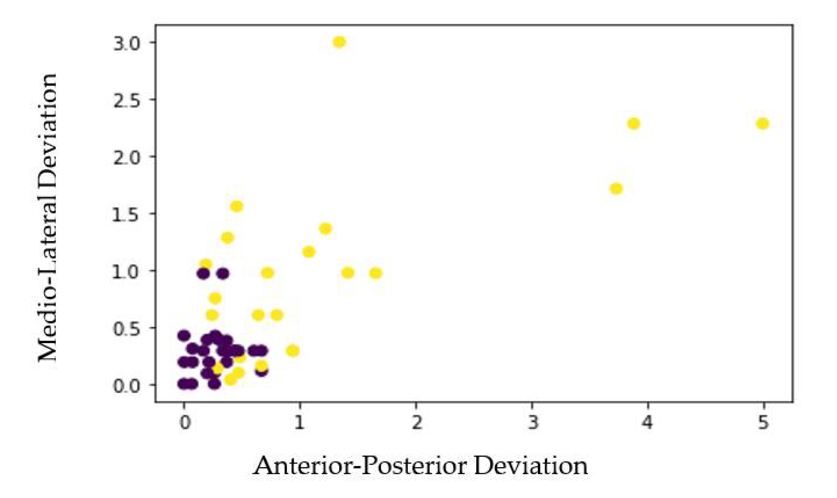
Figure 3.
Data distribution.
Figure 3.
Data distribution.
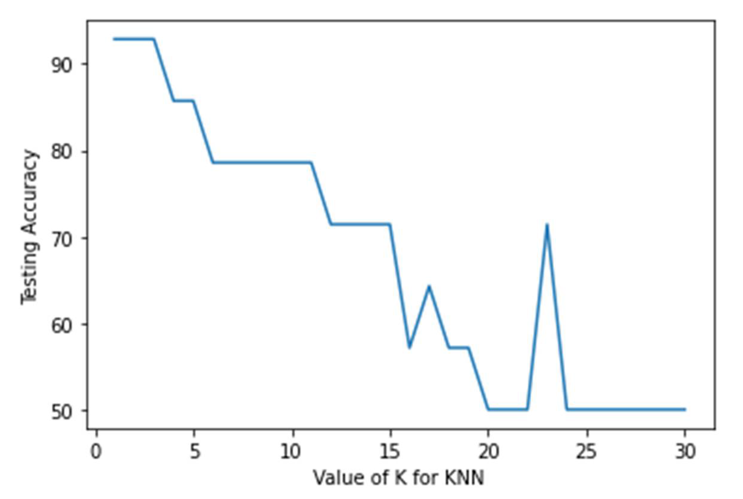
Figure 4.
Variation of testing accuracy vs. value of K.
Figure 4.
Variation of testing accuracy vs. value of K.
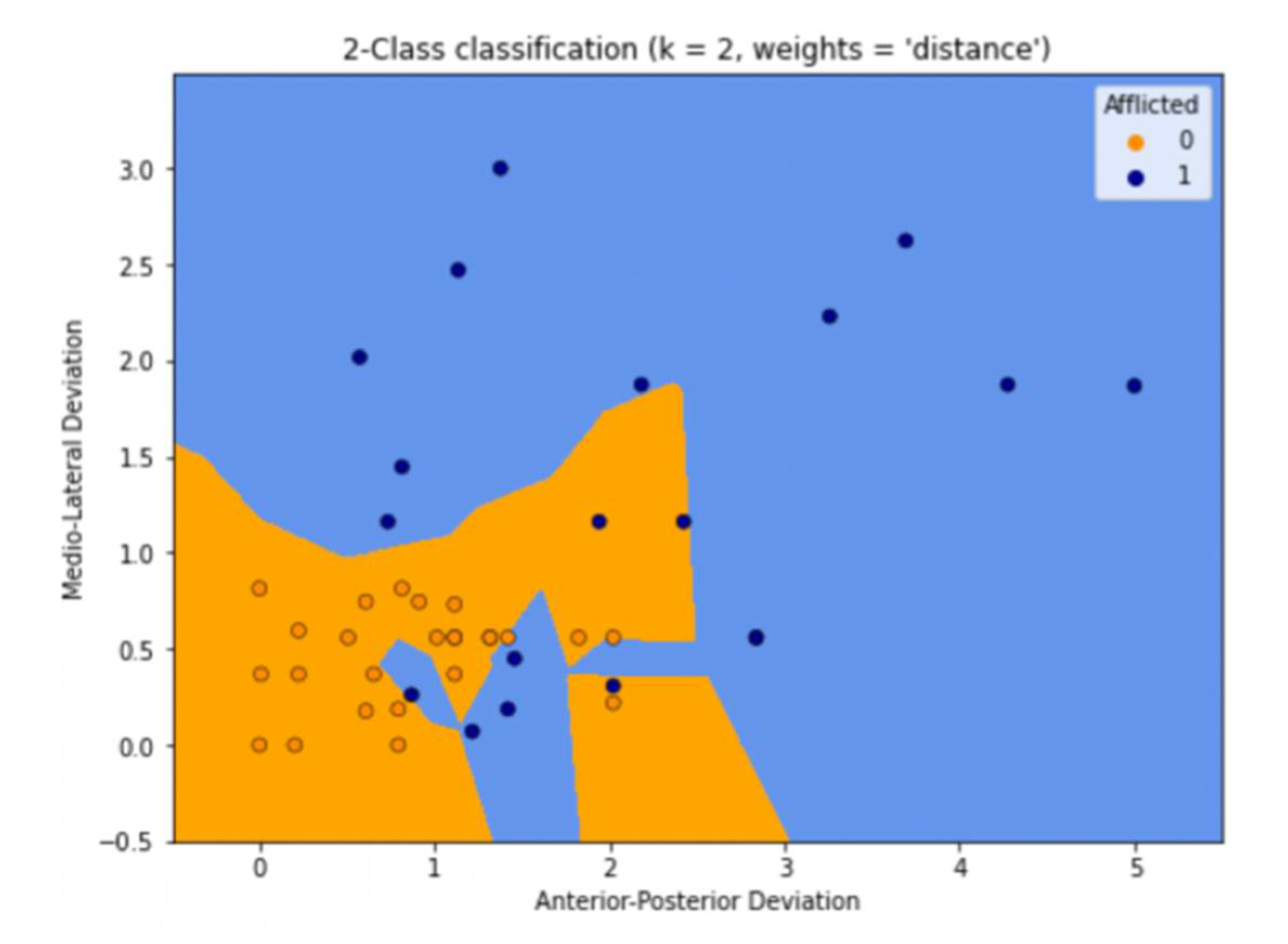
Figure 5.
Prediction using K = 2.
Figure 5.
Prediction using K = 2.
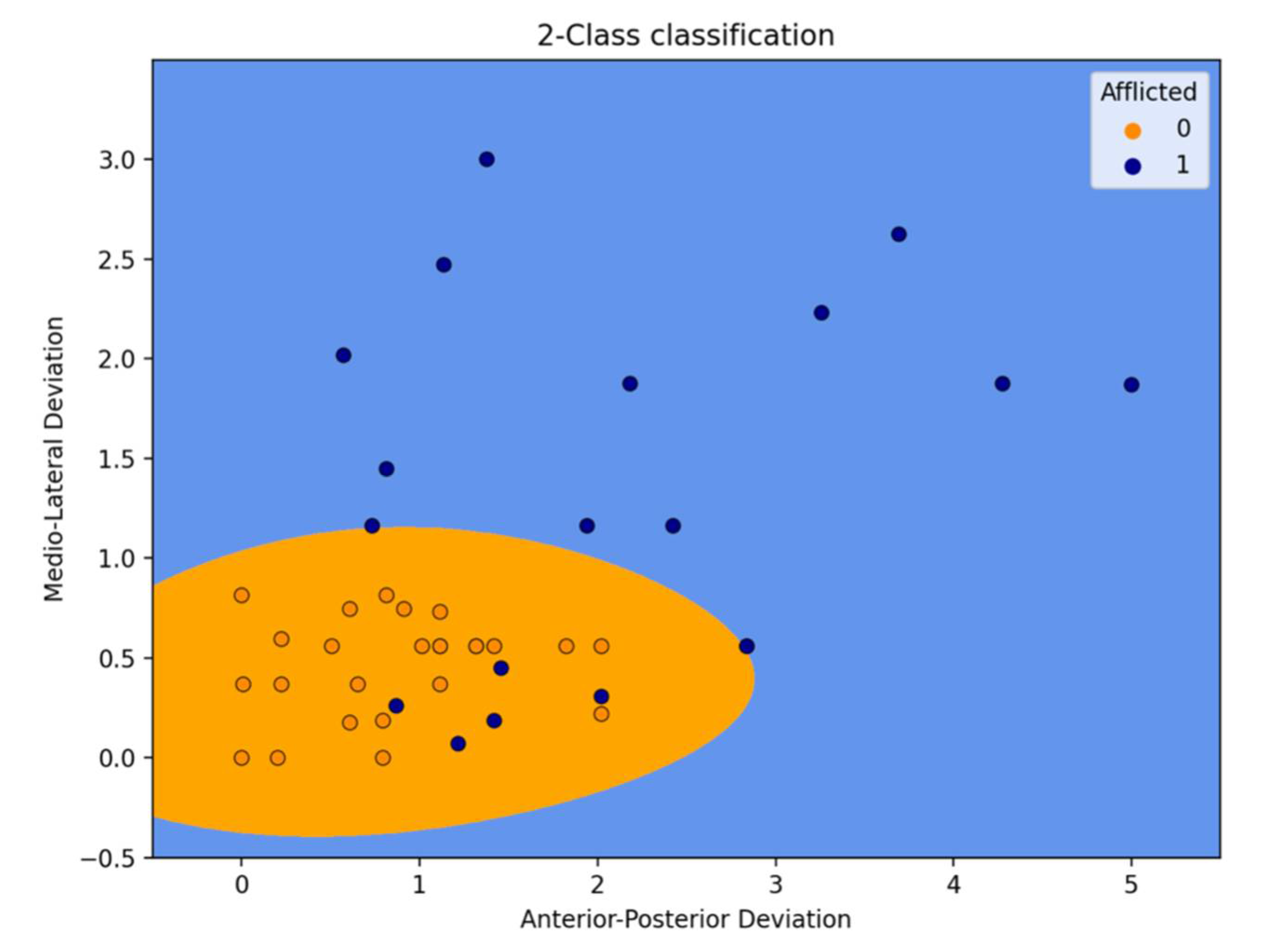
Figure 6.
Prediction as seen on a graph.
Figure 6.
Prediction as seen on a graph.
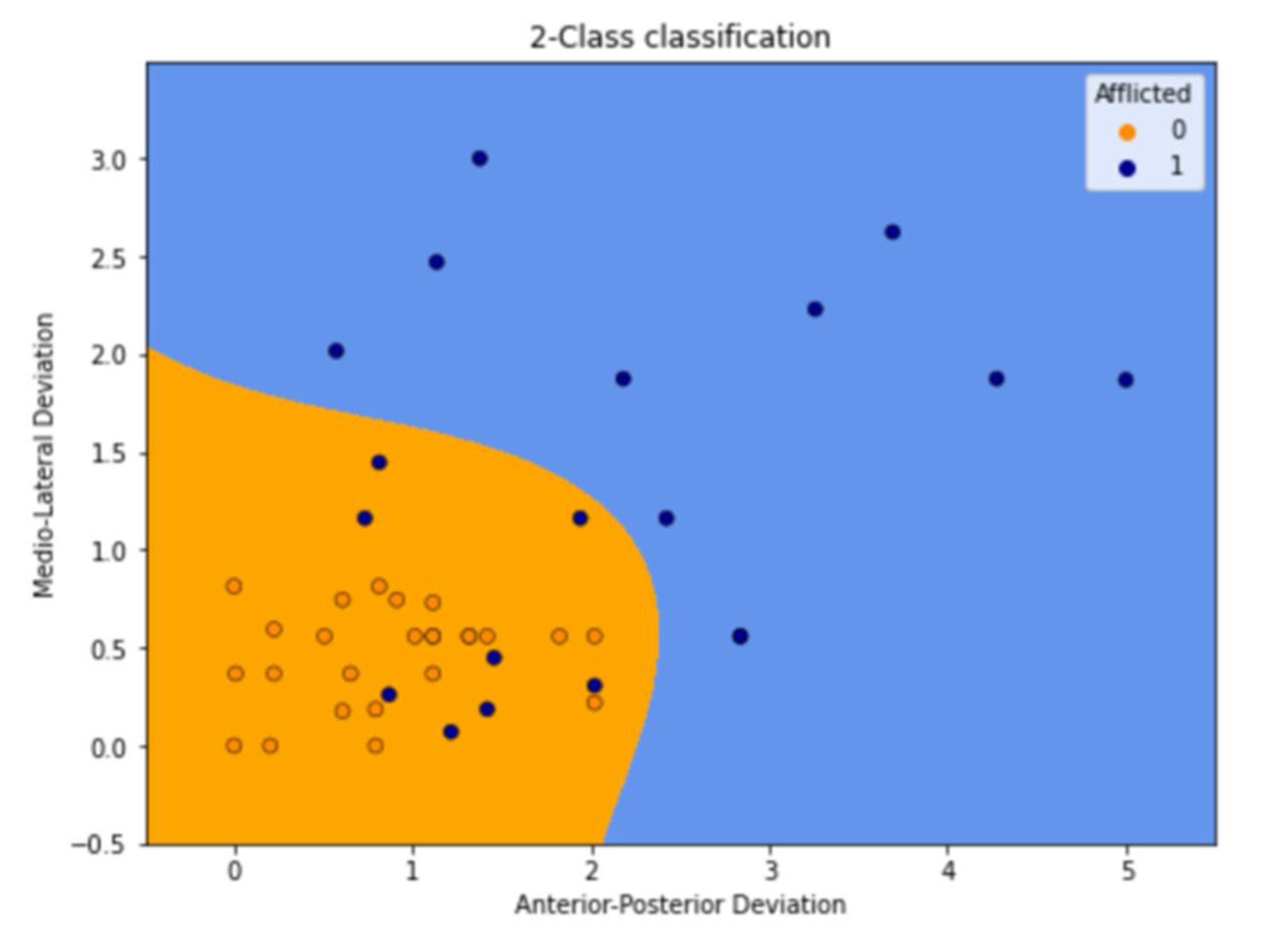
Figure 7.
Prediction as seen on a graph.
Figure 7.
Prediction as seen on a graph.
Figure 8.
Prediction as seen on a graph.
Figure 8.
Prediction as seen on a graph.
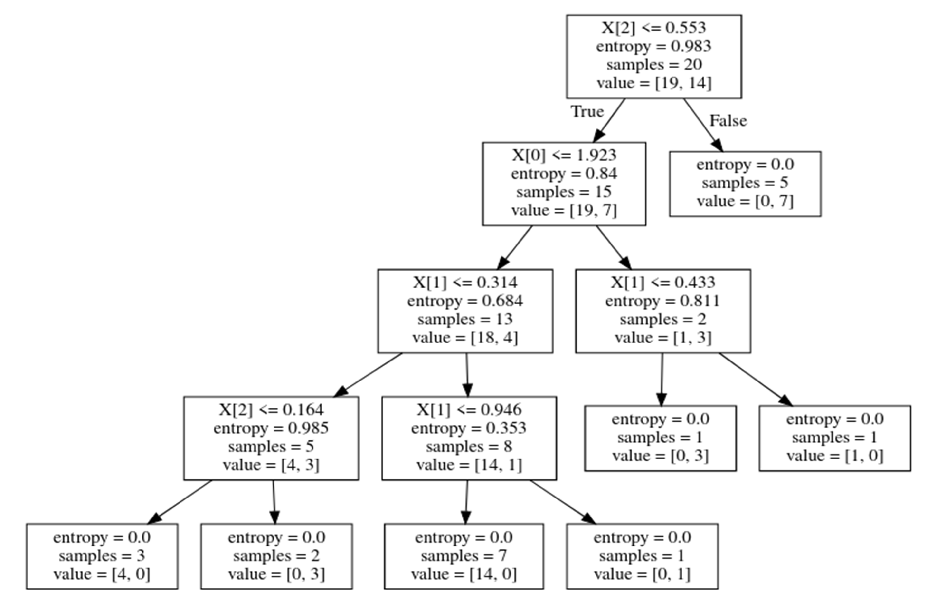
Figure 9.
The Decision Tree with entropy values, where X [0] is AP, X [1] is ML, and X [2] is area under the square.
Figure 9.
The Decision Tree with entropy values, where X [0] is AP, X [1] is ML, and X [2] is area under the square.
Figure 10.
Sample tree 1.
Figure 10.
Sample tree 1.
Figure 11.
Sample tree 2.
Figure 11.
Sample tree 2.
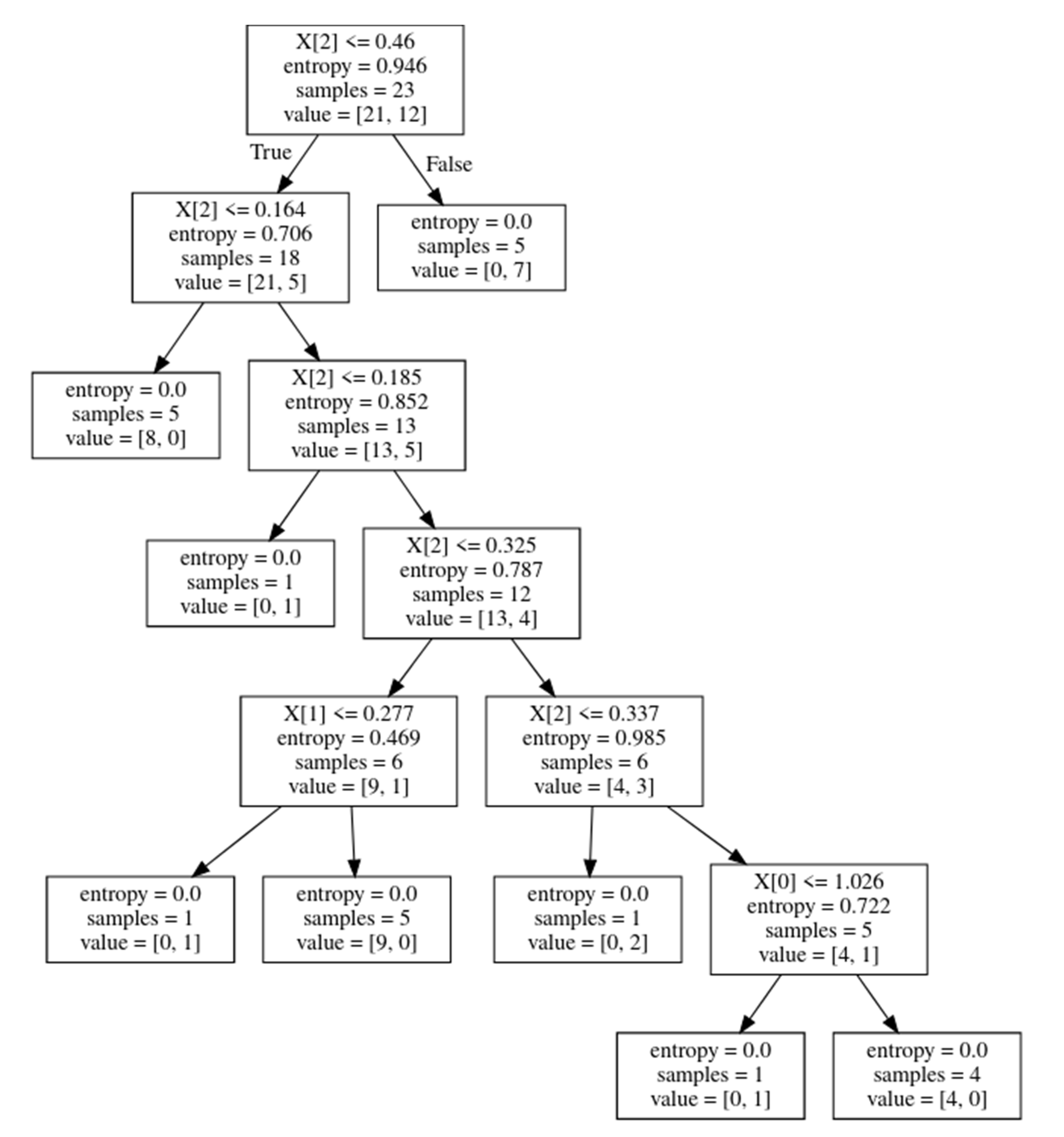
Figure 12.
Sample tree 3, where X [0] is AP, X [1] is ML, and X [2] is area under the square.
Figure 12.
Sample tree 3, where X [0] is AP, X [1] is ML, and X [2] is area under the square.
Table 1.
Performance Metrics for Testing Data.
Table 1.
Performance Metrics for Testing Data.
| | Precision | Recall | F1-Score |
|---|
| 0 | 0.86 | 1.00 | 0.92 |
| 1 | 1.00 | 0.80 | 0.89 |
Table 2.
Performance Metrics for Training Data.
Table 2.
Performance Metrics for Training Data.
| | Precision | Recall | F1-Score |
|---|
| 0 | 1.00 | 1.00 | 0.92 |
| 1 | 1.00 | 0.80 | 0.89 |
Table 3.
Performance Metrics for Testing Data.
Table 3.
Performance Metrics for Testing Data.
| | Precision | Recall | F1-Score |
|---|
| 0 | 0.86 | 1.00 | 0.92 |
| 1 | 1.00 | 0.80 | 0.89 |
Table 4.
Performance Metrics for Training Data.
Table 4.
Performance Metrics for Training Data.
| | Precision | Recall | F1-Score |
|---|
| 0 | 0.79 | 1.00 | 0.88 |
| 1 | 1.00 | 0.64 | 0.78 |
Table 5.
Performance Metrics for Testing Data.
Table 5.
Performance Metrics for Testing Data.
| | Precision | Recall | F1-Score |
|---|
| 0 | 0.86 | 1.00 | 0.92 |
| 1 | 1.00 | 0.80 | 0.89 |
Table 6.
Performance Metrics for Training Data.
Table 6.
Performance Metrics for Training Data.
| | Precision | Recall | F1-Score |
|---|
| 0 | 0.83 | 1.00 | 0.90 |
| 1 | 1.00 | 0.71 | 0.83 |
Table 7.
Performance Metrics for Testing Data.
Table 7.
Performance Metrics for Testing Data.
| | Precision | Recall | F1-Score |
|---|
| 0 | 0.75 | 1.00 | 0.86 |
| 1 | 1.00 | 0.60 | 0.75 |
Table 8.
Performance Metrics for Training Data.
Table 8.
Performance Metrics for Training Data.
| | Precision | Recall | F1-Score |
|---|
| 0 | 0.76 | 1.00 | 0.86 |
| 1 | 1.00 | 0.57 | 0.73 |
Table 9.
Performance Metrics for Testing Data.
Table 9.
Performance Metrics for Testing Data.
| | Precision | Recall | F1-Score |
|---|
| 0 | 1.00 | 0.83 | 0.91 |
| 1 | 0.83 | 1.00 | 0.91 |
Table 10.
Performance Metrics for Training Data.
Table 10.
Performance Metrics for Training Data.
| | Precision | Recall | F1-Score |
|---|
| 0 | 1.00 | 1.00 | 1.00 |
| 1 | 1.00 | 1.00 | 1.00 |
Table 11.
Performance Metrics for Testing Data.
Table 11.
Performance Metrics for Testing Data.
| | Precision | Recall | F1-Score |
|---|
| 0 | 0.86 | 1.00 | 0.92 |
| 1 | 1.00 | 0.80 | 0.89 |
Table 12.
Performance Metrics for Training Data.
Table 12.
Performance Metrics for Training Data.
| | Precision | Recall | F1-Score |
|---|
| 0 | 1.00 | 1.00 | 1.00 |
| 1 | 1.00 | 1.00 | 1.00 |
Table 13.
Validation Accuracy.
Table 13.
Validation Accuracy.
| Classifier | KNN | Logistic Regression | Gaussian Naive Bayes | Support Vector Machine | Decision Tree | Random Forest Classifier |
|---|
| Accuracy | 91% | 91% | 91% | 82% | 91% | 91% |
Table 14.
Training Accuracy.
Table 14.
Training Accuracy.
| Classifier | KNN | Logistic Regression | Gaussian Naive Bayes | Support Vector Machine | Decision Tree | Random Forest Classifier |
|---|
| Accuracy | 100% | 85% | 88% | 82% | 100% | 100% |
Table 15.
Recall based on validation set.
Table 15.
Recall based on validation set.
| Classifier | KNN | Logistic Regression | Gaussian Naive Bayes | Support Vector Machine | Decision Tree | Random Forest Classifier |
|---|
| Recall(0) | 1 | 1 | 1 | 1 | 0.83 | 1 |
| Recall(1) | 0.8 | 0.8 | 0.8 | 0.6 | 1 | 0.8 |


 ,
, 


