Article

Use of Machine Learning for Early Detection of Knee Osteoarthritis and Quantifying Effectiveness of Treatment Using Force Platform

by
Ashish John Prabhakar
1,
Srikanth Prabhu
2,*,
Aayush Agrawal
2,
Siddhisa Banerjee
3,
Abraham M. Joshua
1,
Yogeesh Dattakumar Kamat
4,
Gopal Nath
5 and
Saptarshi Sengupta
6
1
Department of Physiotherapy, Kasturba Medical College, Mangalore, Manipal Academy of Higher Education, Manipal, India
2
Department of Computer Science & Engineering, Manipal Institute of Technology, Manipal Academy of Higher Education, Manipal, India
3
Department of Information Technology, Manipal Institute of Technology, Manipal Academy of Higher Education, Manipal, India
4
Consultant Knee & Hip Surgeon, KMC Hospital, Ambedkar Circle, Mangaluru, Department of Orthopedics, KMC Mangalore MAHE, Manipal, India
5
Department of Mathematics and Statistics, Murray State University, Murray, KY, USA
6
Department of Computer Science, San José State University, San José, CA, USA
*
Author to whom correspondence should be addressed.
J. Sens. Actuator Netw. 2022, 11(3), 48; https://doi.org/10.3390/jsan11030048
Submission received: 24 June 2022 / Revised: 27 July 2022 / Accepted: 27 July 2022 / Published: 23 August 2022

Abstract

:
Knee osteoarthritis is one of the most prevalent chronic diseases. It leads to pain, stiffness, decreased participation in activities of daily living and problems with balance recognition. Force platforms have been one of the tools used to analyse balance in patients. However, identification in early stages and assessing the severity of osteoarthritis using parameters derived from a force plate are yet unexplored to the best of our knowledge. Combining artificial intelligence with medical knowledge can provide a faster and more accurate diagnosis. The aim of our study is to present a novel algorithm to classify the occurrence and severity of knee osteoarthritis based on the parameters derived from a force plate. Forty-four sway movements graphs were measured. The different machine learning algorithms, such as K-Nearest Neighbours, Logistic Regression, Gaussian Naive Bayes, Support Vector Machine, Decision Tree Classifier and Random Forest Classifier, were implemented on the dataset. The proposed method achieves 91% accuracy in detecting sway variation and would help the rehabilitation specialist to objectively identify the patient’s condition in the initial stage and educate the patient about disease progression.

1. Introduction

Knee Osteoarthritis (OA) is one of the most prevalent chronic diseases. It leads to pain, stiffness and decreased participation in activities of daily living [1]. Muscle strength and bony alignment are altered as the joints become deformed, thereby leading to problems with balance recognition (proprioceptive sensory deficit) [2]. Balance involves numerous neuromuscular interactions between the visual, vestibular and neural systems. Any variation in these systems can hence cause balance alterations [3]. Force platforms have been one of the tools used to analyse sway/balance in patients. However, identification of OA in early stages and assessing the severity of OA using parameters derived from force plates are yet unexplored to the best of our knowledge. An accurate and early diagnosis of knee OA by a feature detection algorithm using a force platform, followed by appropriate therapeutic strategies, may help to prevent the progression of the condition.
A force platform, also known as a force plate, is a device that is used to assess dynamic and static posture control and associated gait parameters [4]. There are two types of force platforms: (1) with monoaxial load cells that detect the vertical component of the ground reaction force (FZ), and (2) with load cells that detect the three components of the ground reaction force (FX, FY and FZ) along with the moment of force acting on the multiaxial plates (MX, MY and MZ). Uni- and multiaxial plates can be used to assess the anterior-posterior (AP) and medio-lateral (ML) time series of the centre of pressure (which is a point of application of vertical ground reaction force) over time during a postural test. The Centre of Pressure (COP) is the most commonly used parameter for evaluating postural function. Variations in Centre of Mass (COM) displacements are referred to as body sway, whereas changes in COP position are often referred to as postural sway [5].
Though non-instrumental tests can be used to diagnose motor and sensory disorders, they only provide an overall understanding of how well the posture can be controlled. Instrumented tests such as force plates are required for a thorough and detailed examination of postural balance [5]. For the purpose of this study, the authors employed a dual-axis force plate to measure static postural balance. The aim of our study is to present a novel algorithm to classify the occurrence and severity of knee OA based on the parameters derived from a force plate.

2. Methodology

2.1. Postural Balance Measurement

The subjects required for the present research work were recruited from the specialist department for knee and hip care at KMC Hospital, Ambedkar Circle, Mangalore, India. The study was approved by the institutional ethics committee (ref. no: IECKMCMLR-10/2020/290). Following the recruitment of the subjects based on the inclusion and exclusion criteria, the participants were instructed to stand on the force plate with as much stability as feasible. The inclusion and exclusion criteria are given below:
Inclusion criteria for subjects with EOA:
  • Age ≥20 and <45 years.
  • Satisfying four out of six clinical symptoms criteria (Recurrent pain, Pain following a duration of rest, Discomfort at rest, Swelling, Instability, Reduced range of motion).
  • Subject with clinically and radiologically (Kellgren Lawrence grade 1 or 2) confirmed diagnosis of EOA by an Orthopaedist or a Rheumatologist.
Exclusion criteria:
  • If patient demonstrates any neurological, neuromuscular or musculoskeletal condition other than EOA, RA or other inflammatory arthritis.
  • Obesity (BMI > 30 kg/m2).
  • Subjects with a history of vertigo (vestibular dysfunction).
  • Patients with hypertension.
  • K and L grade 3 and above.
  • Recent surgeries and significant injuries of a lower limb.
The participants were asked to fix their gaze on a mark placed in front of the wall at a distance of 3 m for the open-eye scenario, and the same posture was advocated for the closed-eye scenario. The test was done three times for 30 s each time, with a one-minute break between each attempt [6]. Figure 1 illustrates the entire solution pipeline. Figure 2 represents the session analysis graph and description.

2.2. Pre-Processing

Forty subjects’ sway movements were measured, with twenty-three being afflicted with OA and seventeen without OA.
The following procedure was followed on each of the subjects to formulate the dataset. The AP excursion was found as the absolute difference between the front-most and backward-most points on the graph Figure 2, in terms of percentage over time, with frontward movement as positive and backward movement as negative.
The ML excursion was found as the absolute difference between the leftmost and rightmost points on the graph in terms of percentage over time, with rightward movement as positive and leftward movement as negative. The area under the square was found as the product of the AP and the ML excursions.
Further, the data were augmented by ten non-afflicted points by randomly selecting AP and ML deviations of two unique, non-afflicted subjects. Six outliers were removed from the data to improve accuracy (Figure 3). The data were normalized using maximum–minimum scaling, i.e., the minimum value of a feature was subtracted from that feature of every data point, and the result was divided by the difference between the maximum and minimum values within that feature.
X n e w = X o l d X m i n X m a x X m i n  
Before running the models, the AP excursion, ML excursion and area under the square were given initial weightages in the ratio of 5:3:2, respectively.
The data from the 44 samples were then randomly split into train and test sets in the ratio of 3:1. An additional constant feature called Bias was added to all the data points, with the weightage of 0.5.

3. Results

The following different machine learning algorithms were implemented on the newly augmented dataset.

3.1. K-Nearest Neighbours (KNN)

KNN is a non-parametric supervised machine learning algorithm. The results are approximated locally by only considering k-nearest datasets (based on Euclidean distance) at input each time and predicting their class label (based on the mode of the class labels of the k datasets) [7]. Here, it was used to classify whether the patient suffers from osteoarthritis or not. This algorithm was run for values of k varying from 1 to 30 (number of train samples).
Here, we had three features:
Anterior-posterior (X).
Medio-lateral (Y).
Area under the square (Z).
For a test data sample (X0, Y0, Z0).
The training data sample was as follows: (X0, Y0, Z0),..., (Xn, Yn, Zn).
We calculated the Euclidean distances:
D 1 = ( X 0 X 1 ) 2 + ( Y 0 Y 1 ) 2   + ( Z 0 Z 1 ) 2  
D n   = ( X 0 X n ) 2 + ( Y 0 Y n ) 2   + ( Z 0 Z n ) 2  
Our answer was the class of the dependent variable that had the least Euclidean distance value for k = 1 (wherein we considered only one neighbour).
Similarly, our answer was the class that was the most common in the dependent variables with minimum values of Euclidean distance. The number of values we considered depended on the value of the k set.
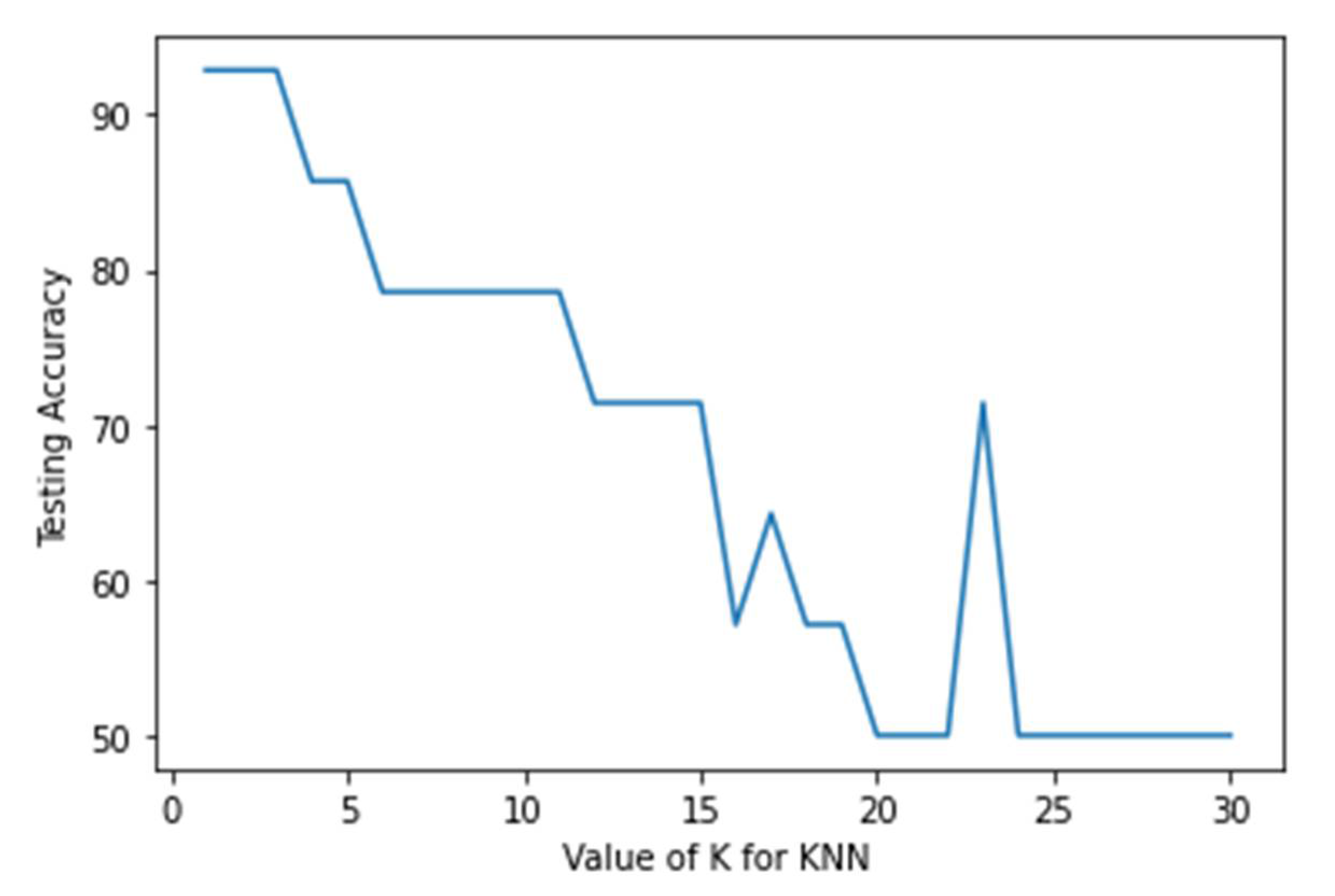
The best results were observed for k = 1, 2, 3 with an accuracy of 92.86%; k = 4, 5 gave an accuracy of 85.71%. The accuracy further decreased with increase in k. the same has been described in Figure 4.
The KNN model performance metrics for the testing and training data are provided below (Table 1 and Table 2). The metrics used for the precision, recall and F1 score is mentioned in Appendix A.
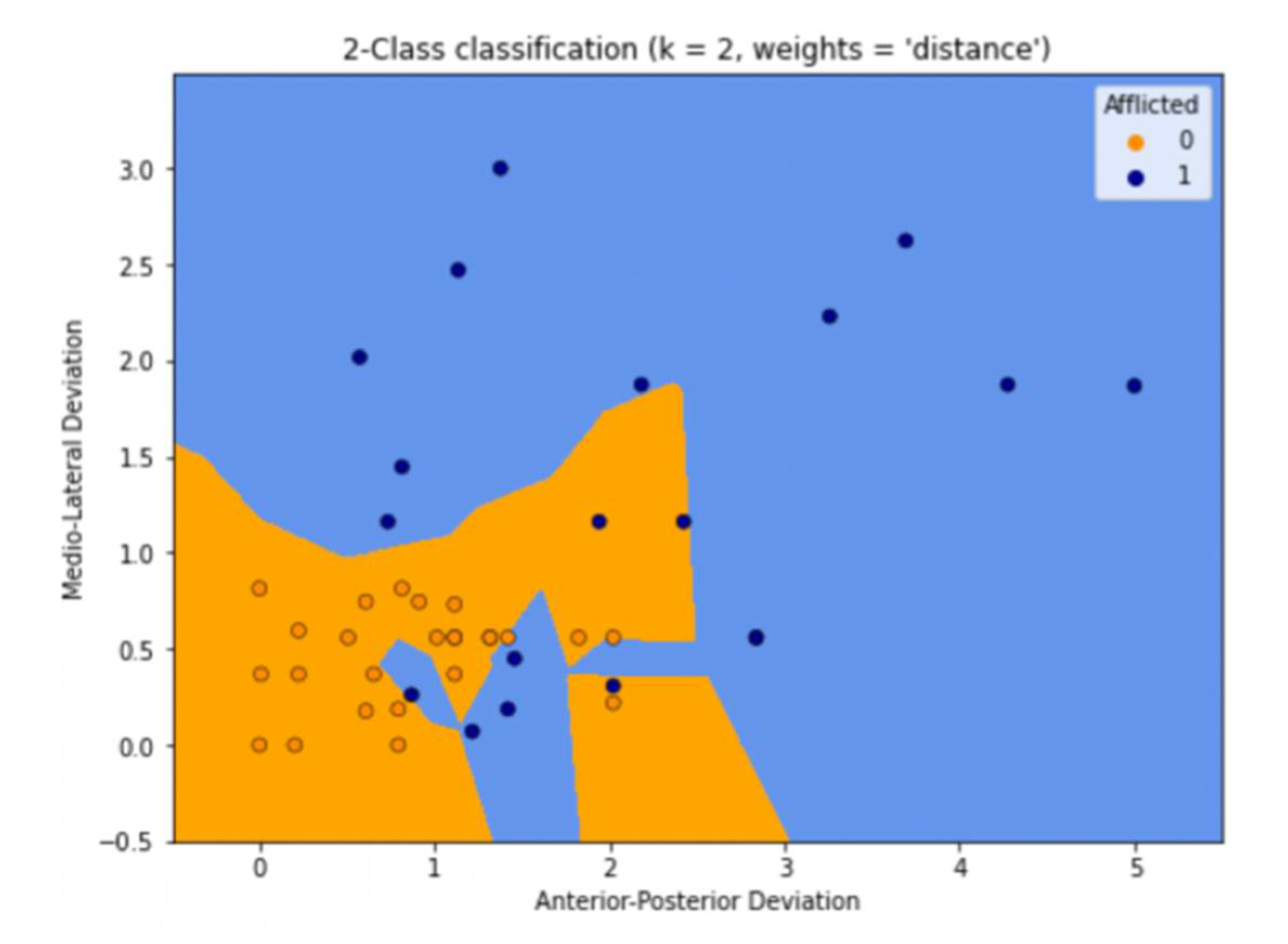
The blue area in Figure 5 indicates what would be predicted as non-afflicted by the machine, and the orange area would be predicted as afflicted.

3.2. Logistic Regression

Logistic Regression (LR) is a statistical machine learning algorithm that is used to model the probability of a particular class. It basically models a logistic or sigmoidal function that best fits our dataset and helps us in classifying [8]. Here, that output was whether the given patient is afflicted by Osteoarthritis or not.
A model was fitted against our dataset, and it gave us the following optimal weights:
AP = 0.73931048 × 5 = 3.6965524.
ML = 1.29462838 × 3 = 3.88388514.
Area = 0.47345805 × 2 = 0.9469161.
Bias = −2.5340467737146395.
The LR model performance metrics for the testing and training data are provided below (Table 3 and Table 4).
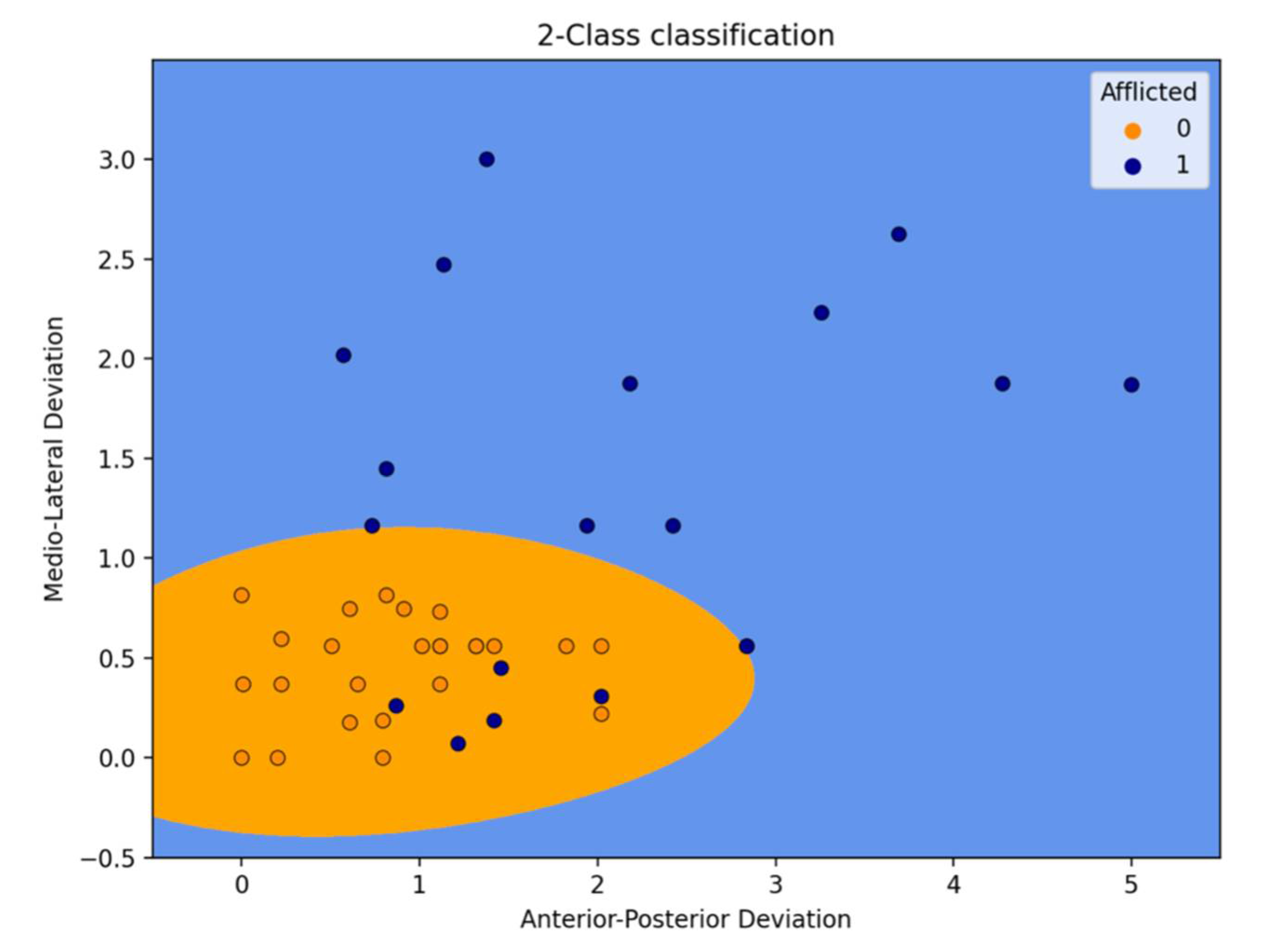
The blue area in Figure 6 indicates what would be predicted as non-afflicted by the machine, and the orange area would be predicted as afflicted.

3.3. Gaussian Naive Bayes

Naive Bayes classifiers are a collection of simple probabilistic classifiers based on applying Bayes’ theorem with strong (naïve) independence assumptions between the features. This is a probabilistic approach towards machine learning. Gaussian Naive Bayes (GNB) is a variant of Naive Bayes. It follows the Gaussian normal distribution and supports continuous data [9].
Data are standardized before implementation, as GNB expects normally distributed data.
The standardization process is given by:
X n e w = X o l d μ σ
where μ = 1 n s a m p l e s   x i = 1 n s a m p l e s X i   is the mean of each feature, and σ = i = 1 n s a m p l e s ( X i μ ) 2 N s a m p l e s   is the standard deviation of that feature.
The GNB model performance metrics for the testing and training data are provided below (Table 5 and Table 6).
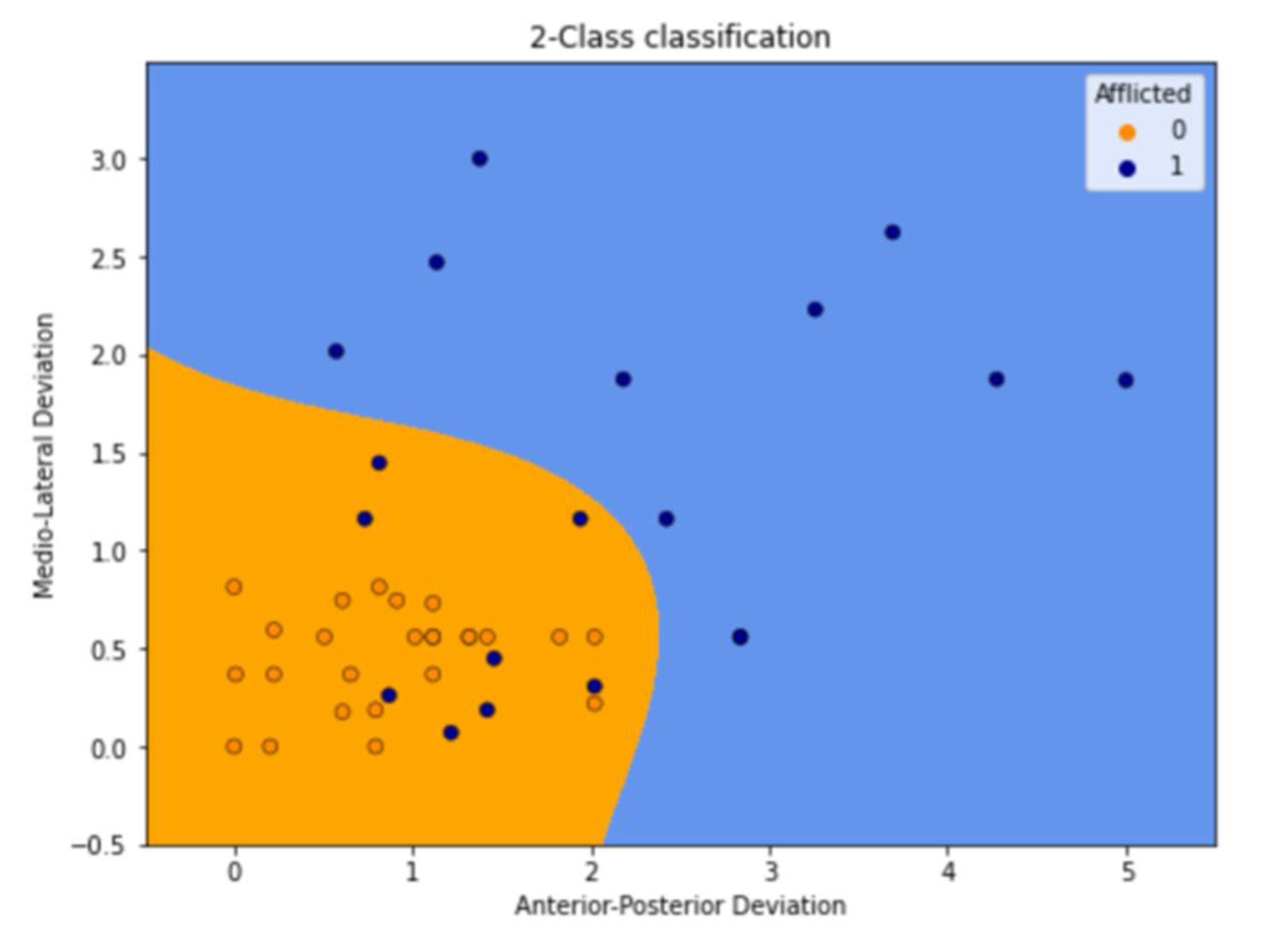
The blue area in Figure 7 indicates what would be predicted as non-afflicted by the machine, and the orange area would be predicted as afflicted.

3.4. Support Vector Machine (SVM)

SVM is an extension of logistic regression concept, but it helps optimise answers for extreme cases. It takes the data point of the extreme cases and uses it as a support. The other training examples become ignorable. Therefore, taking the extreme cases from two different classes, a function is defined that lies at an equal distance from both the extremes, thus increasing the margin for classification so that all the points can be classified as accurately as possible [10]. In the present study, we used a polynomial kernel with the SVM as it yields the best accuracy for the given dataset.
The SVM model performance metrics for the testing and training data are provided below (Table 7 and Table 8).
The blue area in Figure 8 indicates what would be predicted as non-afflicted by the machine, and the orange area would be predicted as afflicted.

3.5. Decision Tree Classifier (DT)

DT is a machine learning algorithm wherein we make the use of tree-like structure to classify the data point. We have nodes that represent certain statements, also known as features (internal nodes), and the lines represent the conditions on those statements (features). Then, the final answer is published on the leaf node [11]. Say, in this case, that it takes AP and asks whether it is over a certain value; then, it creates two branches, and on both branches or on either branch, it either publishes the class or checks another condition on another feature according to the dataset. This continues until the answer is final, and we may or may not exhaust checking all the features. It works best for a large dataset.
The DT model performance metrics for the testing and training data are provided below (Table 9 and Table 10).
The Decision Tree split for our model is represented in Figure 9.

3.6. Random Forest Classifier

A Random Forest (RF) is made up of several individual decision trees that work together to form an ensemble. Each tree in the random forest predicts a class, and the class with the maximum votes is selected as our model’s prediction [12]. It is a meta-estimator that employs averaging to increase predicted accuracy and control over-fitting by fitting a number of decision tree classifiers on various subsamples of the dataset. As it uses multiple trees, the overall accuracy of the algorithm is greater than one decision tree alone [13]. The RF model performance metrics for the testing and training data are provided below (Table 11 and Table 12).
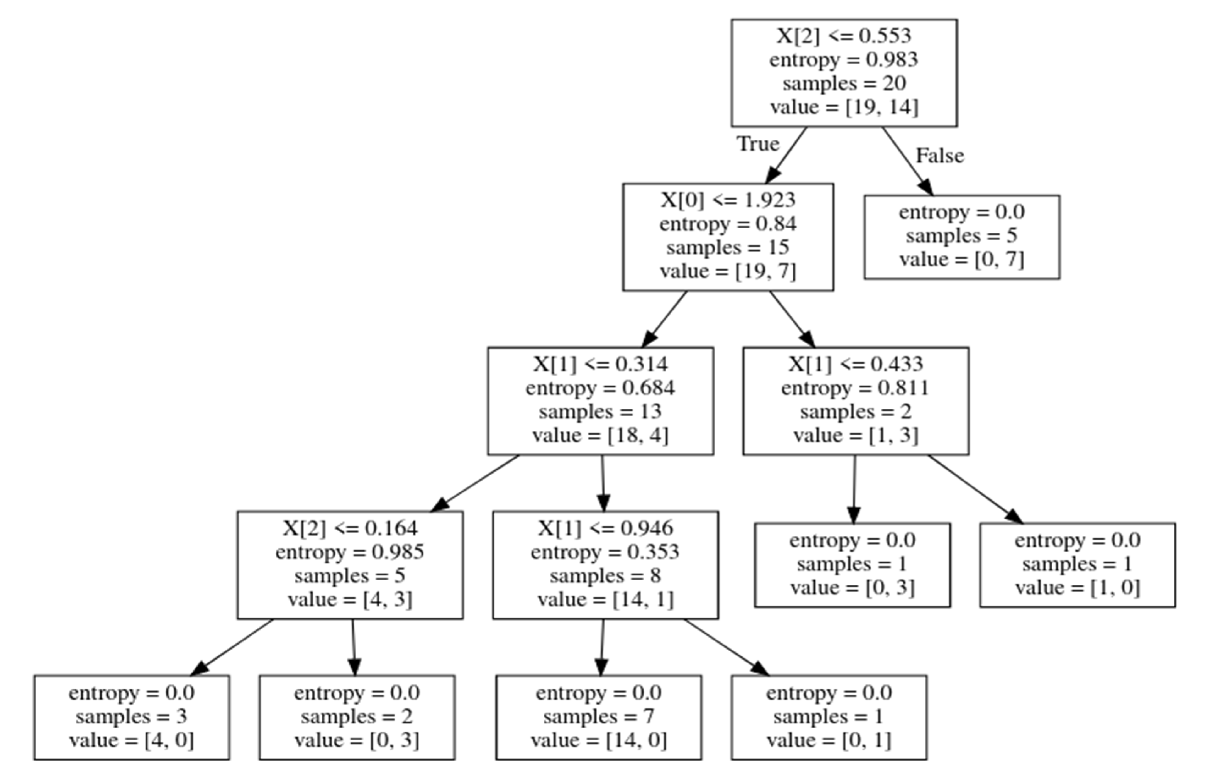
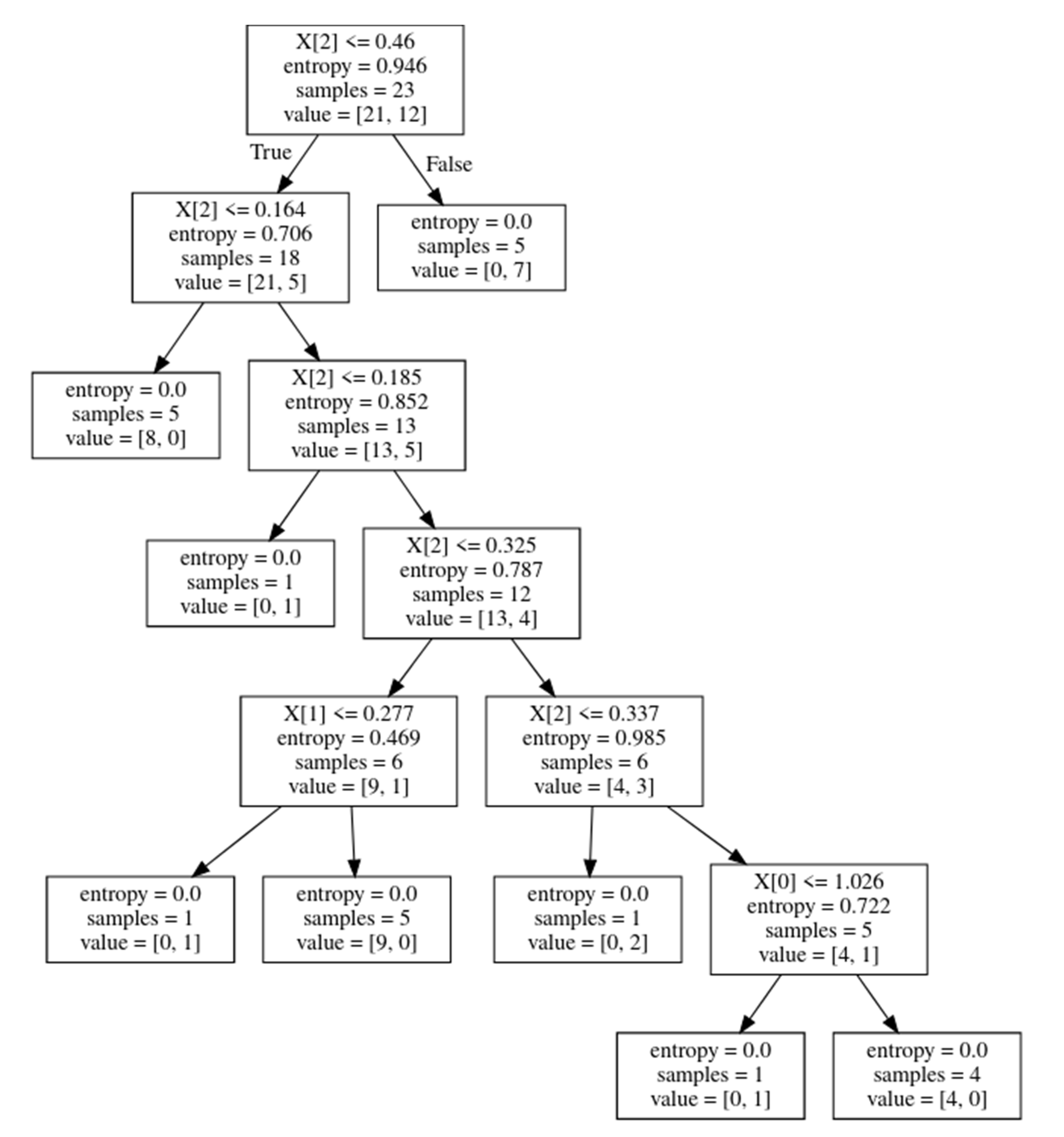
Three sample tree splits from our RF model are represented in Figure 10, Figure 11 and Figure 12. Sample Trees from the Forest:

3.7. Accuracy Summary

The accuracy of the models is compared in the following tables (Table 13 and Table 14).
The recall of the models is compared in the Table 15.

4. Discussion

Importance of Force Plate

A force plate is a mechanical sensing system that is designed to measure ground reaction forces and human moments. Other information that can be procured includes the centre of pressure, the centre of force, and the moment around each of the axes [14]. Current investigative procedures such as Magnetic Resonance Imaging (MRI) and X-rays help to identify the signs of arthritis only after the patient starts showing structural changes. Newer treatments in regenerative medicine are focusing on possibilities of reversing early structural changes to the cartilage tissue that lines the bones within joints [15]. Though MRI can detect early changes by using specific sequences, the availability of such sequences is extremely restricted. Treatment solutions, too, are currently in the research and development phase, and hence, the interventions have not received wide approval.
A force plate being a hyper-sensitive device, it picks up early balance alterations that happen before structural changes develop in patients with early symptoms of the disease. Balance alterations can be rectified with the development of muscular strength using simple exercise techniques at the earlier stages, thereby avoiding operative intervention. It has a potentially huge scope for detecting and preventing progression of one of the commonest diseases—a solution with tremendous public health importance. The entire process consisted mainly of three major steps: Firstly, the collection of osteoarthritic and non-osteoarthritic patients’ data from the hospital; secondly, extracting three main features from the graphical data; and thirdly, running machine learning algorithms on the dataset to come up with the best performing model. The machine learning models have vast applications throughout various fields. According to the findings of the present study, we were able to find that the best models for the early detection of knee osteoarthritis are the KNN Classifier and GNB Classifier. Points on the graph that are nearby are of the same class. The KNN works on the basis of clustering, and hence, it labels nearby points the same, which is the reason for its great performance. GNB is a model that works purely on the basis of probability. Along with giving good results, this model also has the added benefit of giving us an insight, which is that since the model runs well, it is possible that the data of all people are Gaussian in nature (or distributed normally).

5. Conclusions

We propose this method for early detection of knee osteoarthritis. The datasets included a total of 44 graphs. The proposed method achieved 91% accuracy in detecting sway variation. The proposed system would help the rehabilitation specialist to objectively identify the patient’s condition in the initial stage and to educate the patient about disease progression. As a future work, it can be considered to improvise the accuracy of the system towards classifying the patient’s condition into different stages and different compartment involvement as well.

Author Contributions

Conceptualization, A.J.P., Y.D.K. and S.P.; methodology, A.J.P. and Y.D.K.; software, A.A. and S.B.; validation, A.J.P. and Y.D.K.; formal analysis, A.A., S.B. and S.P.; investigation, Y.D.K. and S.P.; resources, Y.D.K. and S.P.; data curation, A.J.P., A.A and S.B; writing—original draft preparation, A.J.P., A.M.J., A.A. and Y.D.K.; writing—review and editing, A.J.P., A.M.J., Y.D.K. and G.N; supervision, Y.D.K. and S.P.; project administration, Y.D.K., S.P, G.N. and S.S., funding acquisition, nil. All authors have read and agreed to the published version of the manuscript.

Funding

The authors received no direct funding for this research.

Institutional Review Board Statement

The Institutional Ethics Committee, Kasturba Medical College, Mangalore (ref. no: IECKMCMLR-10/2020/290. Date of approval: 22 October 2020).

Informed Consent Statement

Informed consent was obtained from all subjects involved in the study.

Conflicts of Interest

The authors declare no conflict of interest.

Abbreviation

OAOsteoarthritis
MLMedio-lateral
APAnterior-posterior
COPCentre of pressure
KNNK-Nearest Neighbours
LRLogistic Regression
SVMSupport Vector Machine
GNBGaussian Naive Bayes
DTDecision Tree Classifier
TPTrue positive
FPFalse positive
TNTrue negative
FNFalse negative

Appendix A

Metrics Used:
ref: TP = True positive; FP = False positive; TN = True negative; FN = False negative
Accuracy: Accuracy is a metric for evaluating classification models. Accuracy is the fraction of predictions that our model correctly predicted. It also has the following definition:
Accuracy = (Number of correct predictions)/ (Total number of predictions)
In the case of binary classification, accuracy is also calculated in terms of positives and negatives, which is given as follows:
Accuracy = (TP + TN)/(TP + TN + FP + FN)
Precision: Precision (positive predictive value) gives the proportion of positive identifications that are actually correct.
Precision = (TP)/(TP + FP)
Recall: Recall gives the proportion of actual positives that were identified correctly.
Recall = (TP)/(TP + FN)
F1 score: In the calculation of F-score/F1-score, the precision and recall of the model are combined, and it is defined as the harmonic mean of the model’s precision and recall. The formula for the standard F1-score is
F1-score = 2/((1/recall) + (1/precision)) = 2 × ((recall × precision)/(recall + precision)) = TP/(TP + 0.5 × (FP + FN))
Support: The support is the number of samples of the true response that lie in that class.
Macro avg: The method is straightforward, where we simply have to take the average of the precision and recall of the system on various different sets. The Macro-average F-Score is the harmonic mean of these two figures. Macro-average method can be used when we want to know the overall performance of the system across various sets of data. No specific decision is drawn from this average.
Weighted avg: Weighted average takes into consideration the number of each class present in its calculation. The lower the number of one class, the lower the impact its precision/recall/F1 score has on the weighted average for each of those things.

References

  1. Lawson, T.; Morrison, A.; Blaxland, S.; Wenman, M.; Schmidt, C.G.; Hunt, M.A. Laboratory-based measurement of standing balance in individuals with knee osteoarthritis: A systematic review. Clin. Biomech. 2015, 30, 330–342. [Google Scholar] [CrossRef] [PubMed]
  2. Hatfield, G.L.; Morrison, A.; Wenman, M.; Hammond, C.A.; Hunt, M.A. Clinical Tests of Standing Balance in the Knee Osteoarthritis Population: Systematic Review and Meta-analysis. Phys. Ther. 2016, 96, 324–337. [Google Scholar] [CrossRef] [PubMed] [Green Version]
  3. Liu, C.; Wan, Q.; Zhou, W.; Feng, X.; Shang, S. Factors associated with balance function in patients with knee osteoarthritis: An integrative review. Int. J. Nurs. Sci. 2017, 4, 402–409. [Google Scholar] [CrossRef] [PubMed]
  4. Whittle, M. Gait Analysis: An Introduction, 4th ed.; Butterworth-Heinemann: Oxford, UK, 2007; p. 160. [Google Scholar]
  5. Paillard, T.; Noé, F. Techniques and Methods for Testing the Postural Function in Healthy and Pathological Subjects. BioMed Res. Int. 2015, 2015, 891390. [Google Scholar] [CrossRef] [PubMed] [Green Version]
  6. Taglietti, M.; Bela, L.F.D.; Dias, J.M.; Pelegrinelli, A.R.M.; Nogueira, J.F.; Júnior, J.P.B.; da Sivla Carvalho, R.G.; McVeigh, J.G.; Facci, L.M.; Moura, F.A.; et al. Postural Sway, Balance Confidence, and Fear of Falling in Women with Knee Osteoarthritis in Comparison to Matched Controls. PM R J. Inj. Funct. Rehabil. 2017, 9, 774–780. [Google Scholar] [CrossRef] [PubMed]
  7. Peterson, L.E. K-nearest neighbor. Scholarpedia 2009, 4, 1883. [Google Scholar] [CrossRef]
  8. Wright, R.E. Logistic regression. In Reading and Understanding Multivariate Statistics; Grimm, L.G., Yarnold, P.R., Eds.; American Psychological Association: Washington, DC, USA, 1995; pp. 217–244. [Google Scholar]
  9. Rish, I.; An empirical study of the naive bayes classifier. In IJCAI, Workshop on Empirical Methods in Artificial Intelligence; 2001; Volume 3, pp. 41–46. Available online: http://citeseerx.ist.psu.edu/viewdoc/summary?doi=10.1.1.330.2788 (accessed on 23 June 2022).
  10. Noble, W.S. What is a support vector machine? Nat. Biotechnol. 2006, 24, 1565–1567. [Google Scholar] [CrossRef] [PubMed]
  11. Safavian, S.R.; Landgrebe, D. A survey of decision tree classifier methodology. IEEE Trans. Syst. Man Cybern. 1991, 21, 660–674. [Google Scholar] [CrossRef] [Green Version]
  12. Pal, M. Random forest classifier for remote sensing classification. Int. J. Remote Sens. 2007, 26, 217–222. [Google Scholar] [CrossRef]
  13. Prajwala, T.R. A Comparative Study on Decision Tree and Random Forest Using R Tool. Int. J. Adv. Res. Comput. Commun. Eng. 2015, 4, 196–199. [Google Scholar] [CrossRef]
  14. Lamkin-Kennard, K.A.; Popovic, M.B. 4-Sensors: Natural and Synthetic Sensors in Biomechanics, 1st ed.; Academic Press: Cambridge, MA, USA, 2019; pp. 81–107. [Google Scholar] [CrossRef]
  15. Duffell, L.D.; Southgate, D.F.L.; Gulati, V.; McGregor, A.H. Balance and gait adaptations in patients with early knee osteoarthritis. Gait Posture 2014, 39, 1057–1061. [Google Scholar] [CrossRef] [Green Version]
Figure 1. Solution Architecture of the ensemble Machine Learning algorithms.
Jsan 11 00048 g001
Figure 2. Force plate session analysis graph and parameter description.
Jsan 11 00048 g002
Figure 3. Data distribution.
Jsan 11 00048 g003
Figure 4. Variation of testing accuracy vs. value of K.
Jsan 11 00048 g004
Figure 5. Prediction using K = 2.
Jsan 11 00048 g005
Figure 6. Prediction as seen on a graph.
Jsan 11 00048 g006
Figure 7. Prediction as seen on a graph.
Jsan 11 00048 g007
Figure 8. Prediction as seen on a graph.
Jsan 11 00048 g008
Figure 9. The Decision Tree with entropy values, where X [0] is AP, X [1] is ML, and X [2] is area under the square.
Jsan 11 00048 g009
Figure 10. Sample tree 1.
Jsan 11 00048 g010
Figure 11. Sample tree 2.
Jsan 11 00048 g011
Figure 12. Sample tree 3, where X [0] is AP, X [1] is ML, and X [2] is area under the square.
Jsan 11 00048 g012
Table 1. Performance Metrics for Testing Data.
PrecisionRecallF1-Score
00.861.000.92
11.000.800.89
Testing Accuracy: 91%.
Table 2. Performance Metrics for Training Data.
PrecisionRecallF1-Score
01.001.000.92
11.000.800.89
Training Accuracy: 100%.
Table 3. Performance Metrics for Testing Data.
PrecisionRecallF1-Score
00.861.000.92
11.000.800.89
Testing Accuracy: 91%.
Table 4. Performance Metrics for Training Data.
PrecisionRecallF1-Score
00.791.000.88
11.000.640.78
Training Accuracy: 85%.
Table 5. Performance Metrics for Testing Data.
PrecisionRecallF1-Score
00.861.000.92
11.000.800.89
Testing Accuracy: 91%.
Table 6. Performance Metrics for Training Data.
PrecisionRecallF1-Score
00.831.000.90
11.000.710.83
Training Accuracy: 88%.
Table 7. Performance Metrics for Testing Data.
PrecisionRecallF1-Score
00.751.000.86
11.000.600.75
Testing Accuracy: 82%.
Table 8. Performance Metrics for Training Data.
PrecisionRecallF1-Score
00.761.000.86
11.000.570.73
Training Accuracy: 88%.
Table 9. Performance Metrics for Testing Data.
PrecisionRecallF1-Score
01.000.830.91
10.831.000.91
Testing Accuracy: 91%.
Table 10. Performance Metrics for Training Data.
PrecisionRecallF1-Score
01.001.001.00
11.001.001.00
Training Accuracy: 100%.
Table 11. Performance Metrics for Testing Data.
PrecisionRecallF1-Score
00.861.000.92
11.000.800.89
Testing Accuracy: 91%.
Table 12. Performance Metrics for Training Data.
PrecisionRecallF1-Score
01.001.001.00
11.001.001.00
Training Accuracy: 100%.
Table 13. Validation Accuracy.
ClassifierKNNLogistic RegressionGaussian Naive BayesSupport Vector MachineDecision TreeRandom Forest Classifier
Accuracy91%91%91%82%91%91%
Table 14. Training Accuracy.
ClassifierKNNLogistic RegressionGaussian Naive BayesSupport Vector MachineDecision TreeRandom Forest Classifier
Accuracy100%85%88%82%100%100%
Table 15. Recall based on validation set.
ClassifierKNNLogistic RegressionGaussian Naive BayesSupport Vector MachineDecision TreeRandom Forest Classifier
Recall(0)11110.831
Recall(1)0.80.80.80.610.8
Publisher’s Note: MDPI stays neutral with regard to jurisdictional claims in published maps and institutional affiliations.