
Multi-Camera Extrinsic Calibration for Real-Time Tracking in Large Outdoor Environments

 ,
,  , , ,
, , ,  and
and
Abstract
:1. Introduction
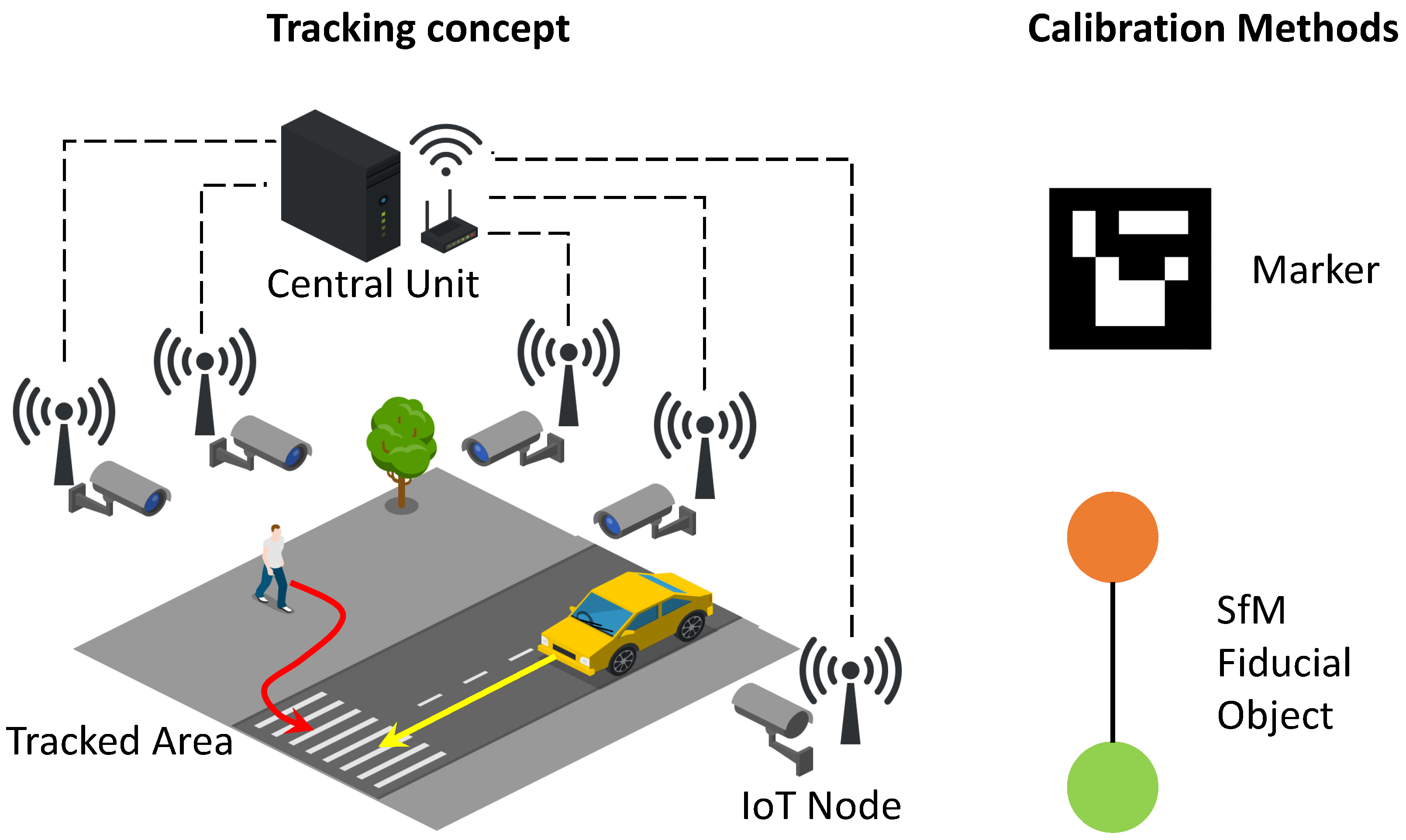
- Distributed IoT node architecture for synchronized visual perception of the environment;
- A comparison of camera calibration algorithms, the former marker-based and the latter based on SfM;
- A novel and simple calibration tool for the SfM technique.
2. State of the Art
Problem Statement
3. Background on Camera Models
3.1. Intrinsic Calibration with Pinhole Cameras
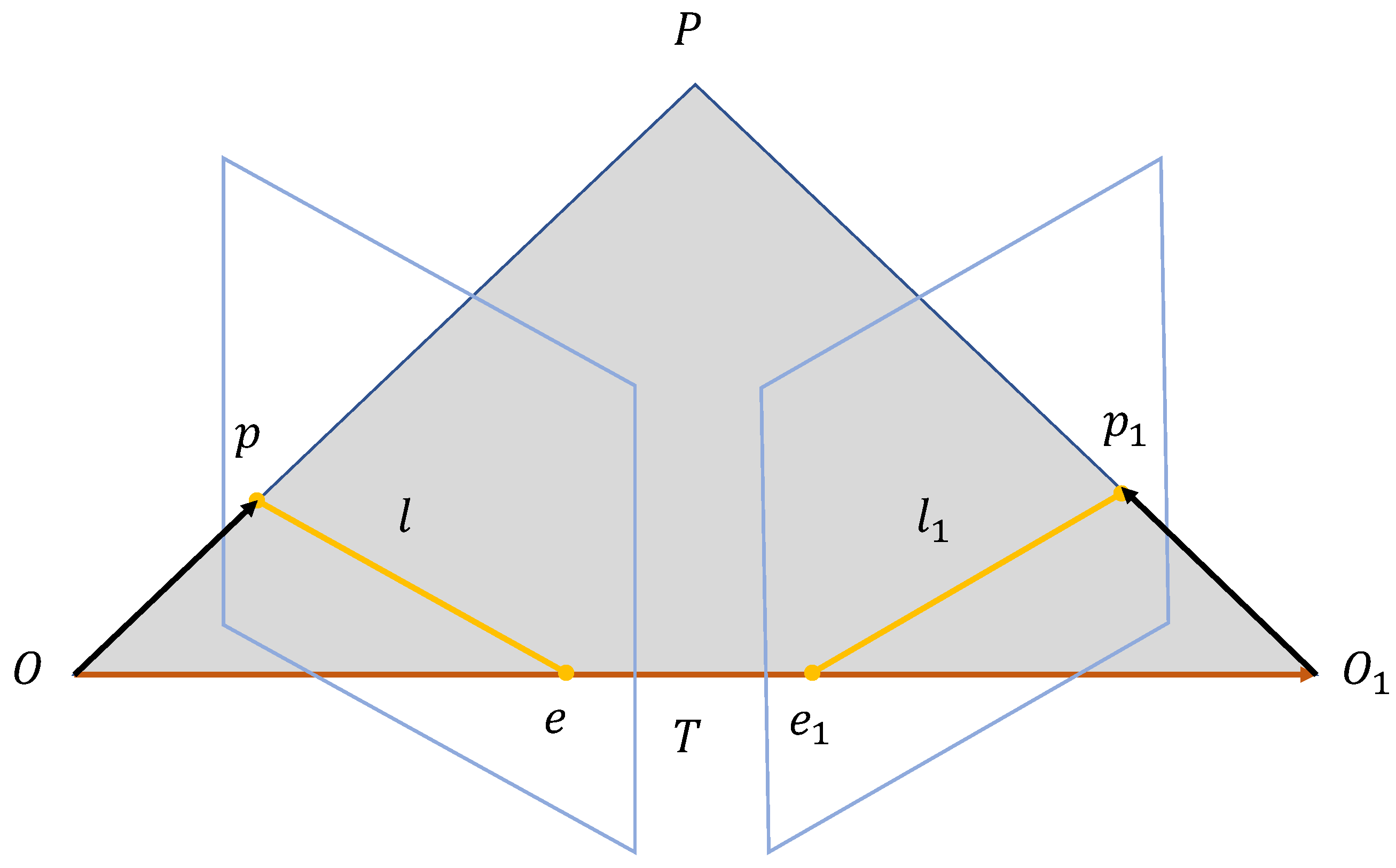
3.2. Epipolar Geometry and Essential Matrices
3.3. Outliers Removal with RANSAC
3.4. Motion Estimation
- and
- and
- and
- and
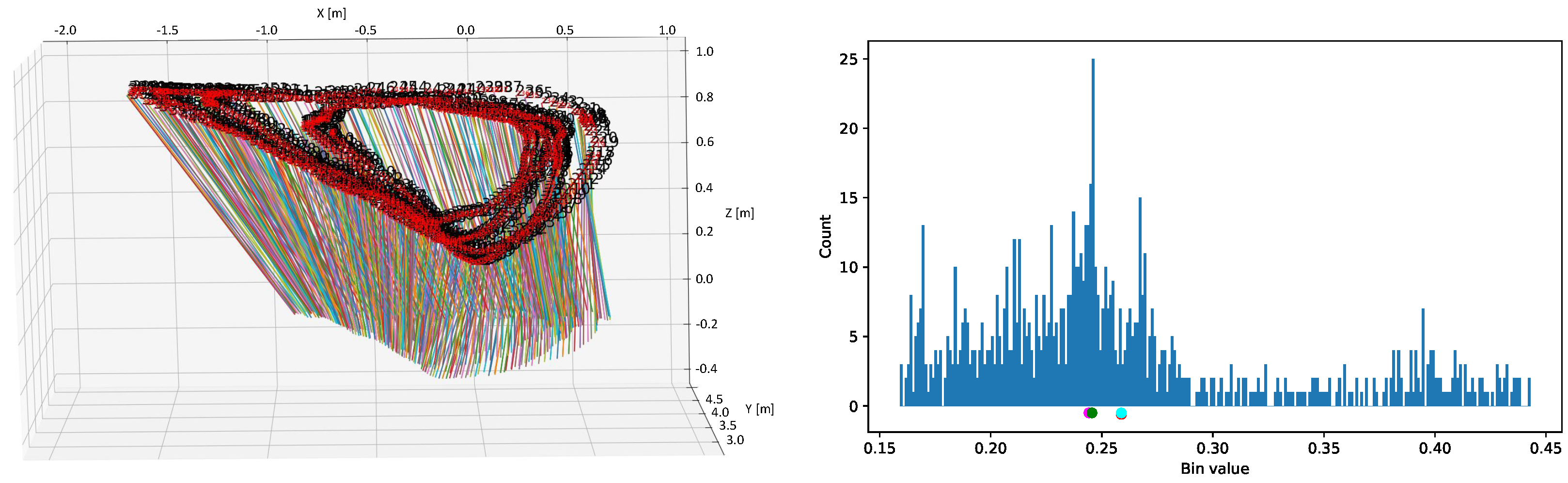
3.5. Scale Determination
4. Methods
4.1. Marker-Based Camera Pose Estimation
4.2. SFM-Based Camera Pose Estimation
- Feature extraction
- Feature matching/tracking
- Outlier removal
- Motion/Pose estimation
- Bundle adjustments
4.2.1. Feature Extraction
4.2.2. Feature Matching
4.2.3. Pose Estimation
4.2.4. Bundle Adjustments
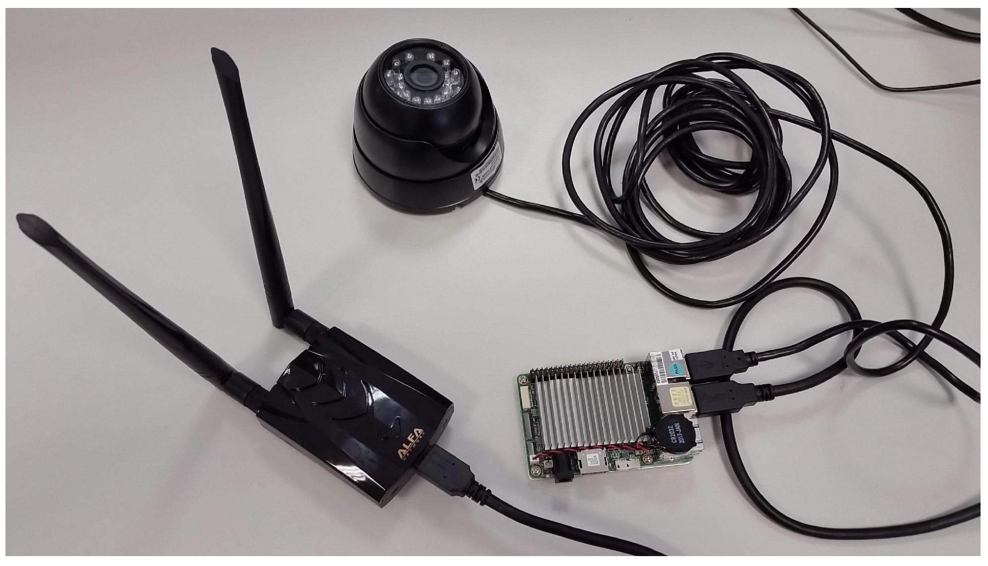
4.3. IoT Camera Nodes
4.3.1. Software System
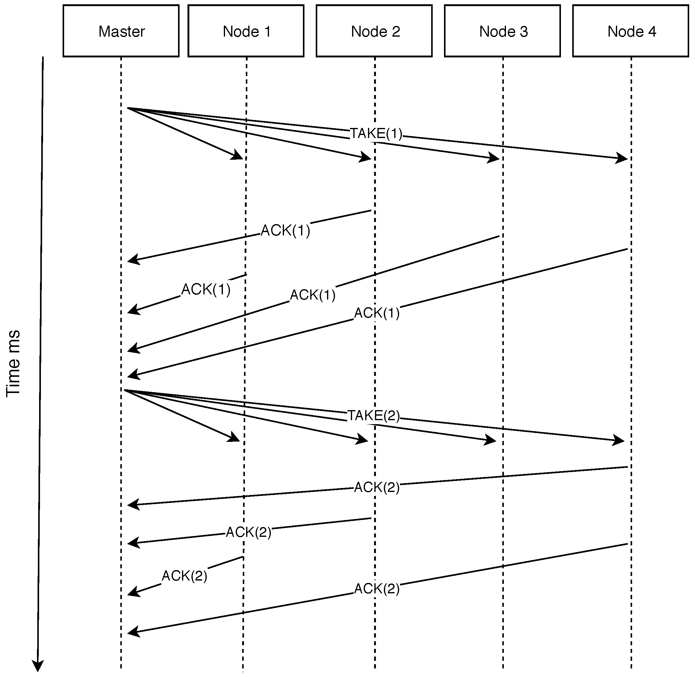
4.3.2. Synchronization Algorithm
- The user sets a number N of images requested to be taken by each camera;
- A TAKE(i) message is broadcast from the master to the nodes, triggering the acquisition of a frame;
- An acknowledgment message (ACK) is sent by each node to the master after the acquisition;
- The master waits for the ACK message to be received from each node, then it broadcasts a TAKE(i+1) message;
- Steps 2 to 4 are repeated until N desired number of acquisitions are reached.
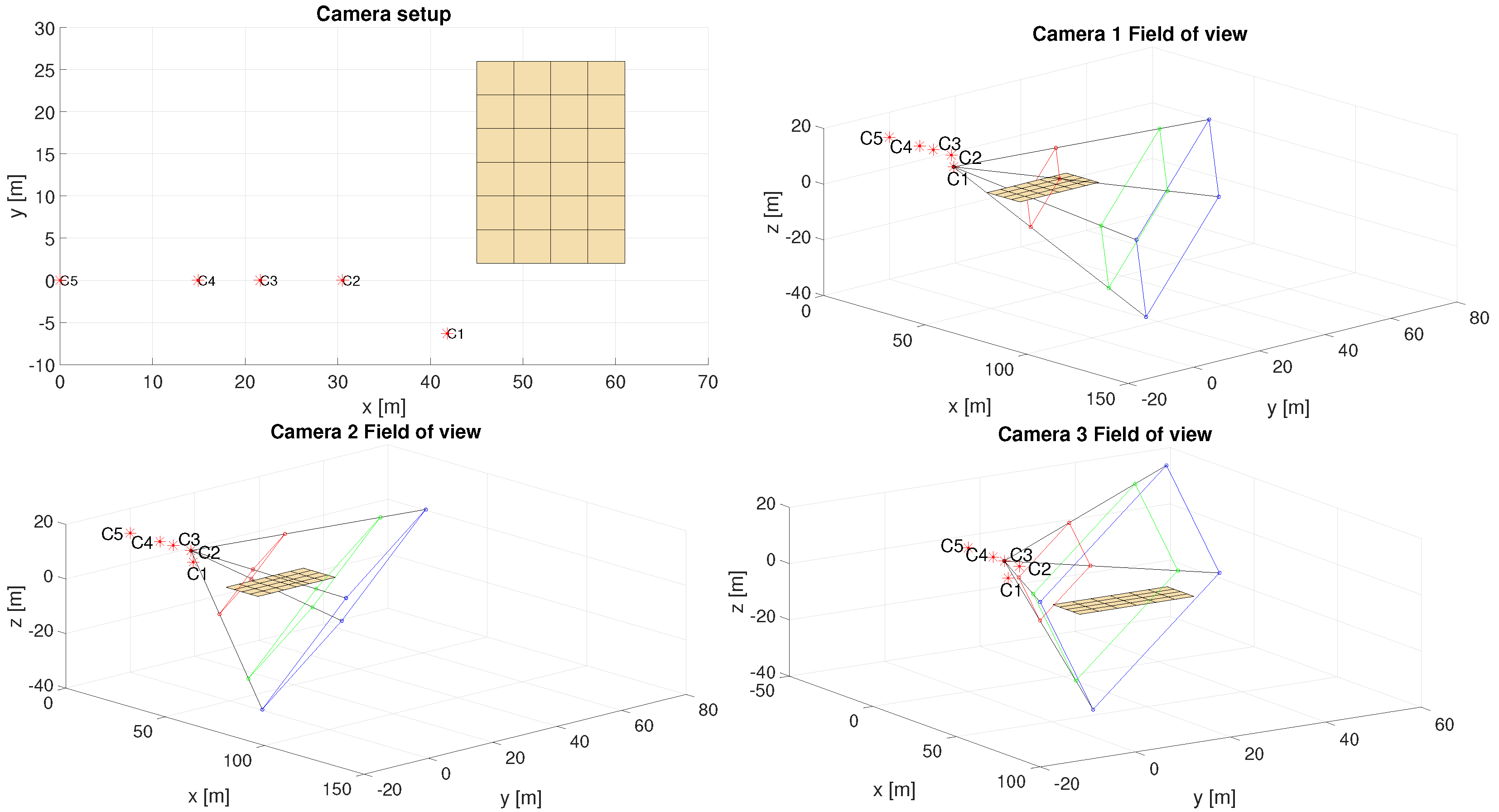
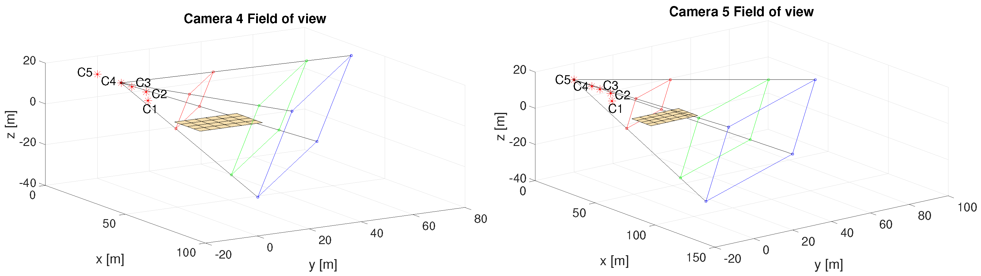
5. Testing Environments and Setups
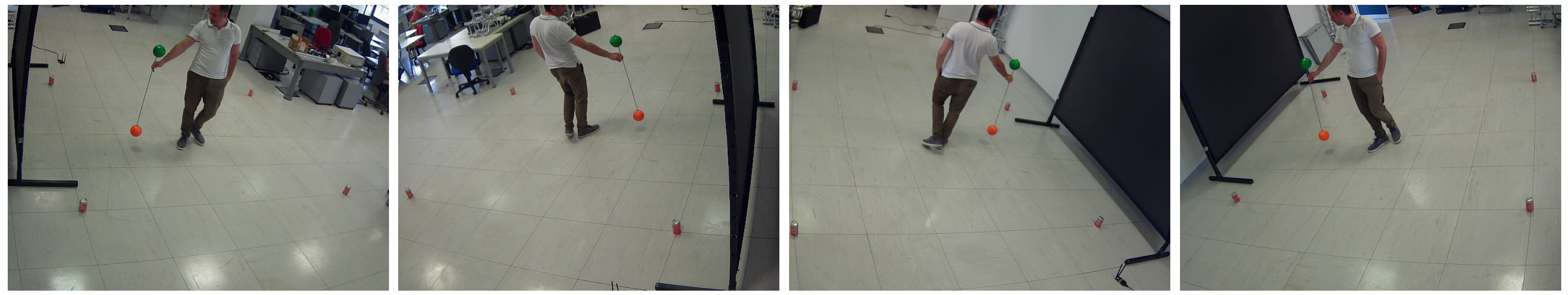
5.1. Indoor Setup
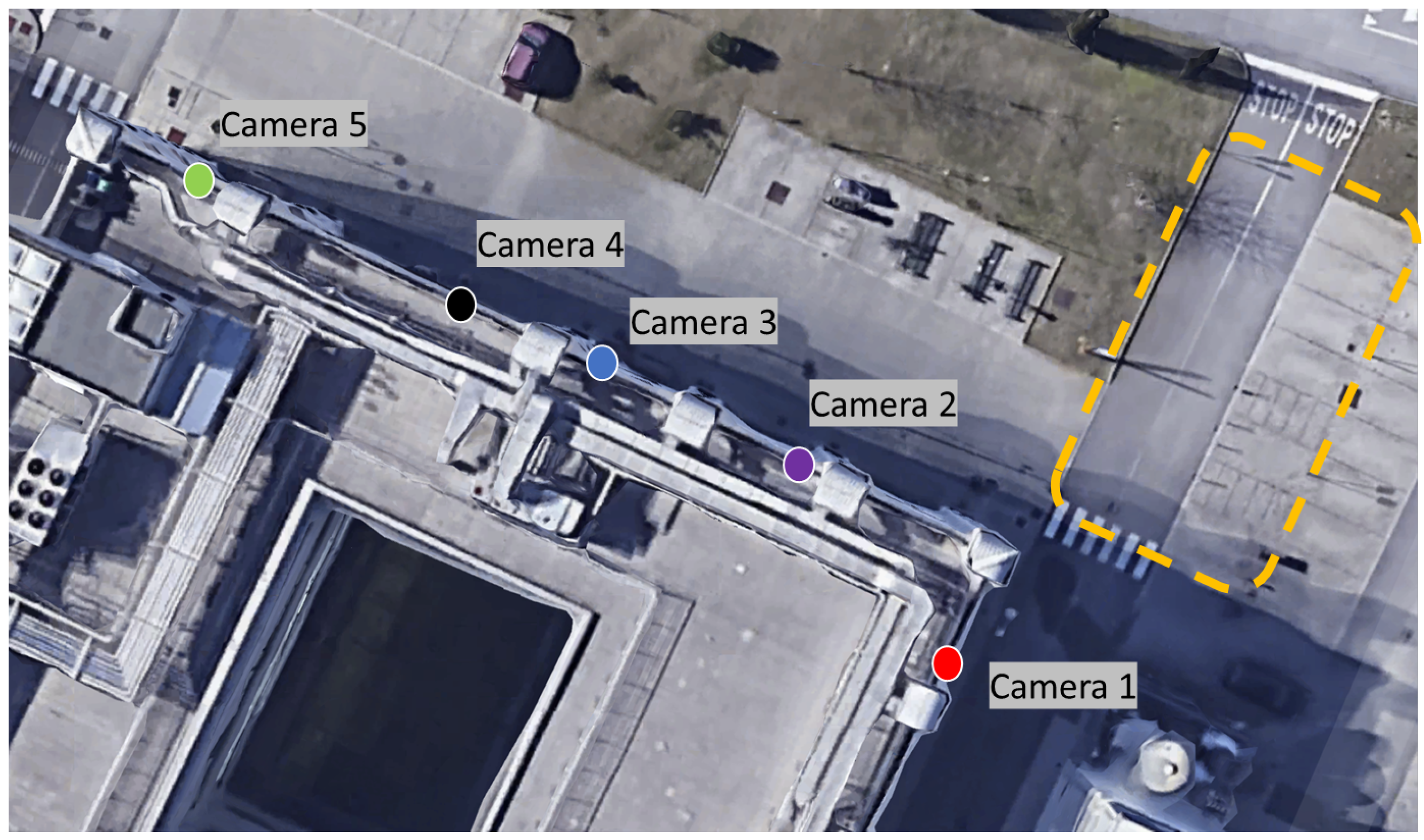
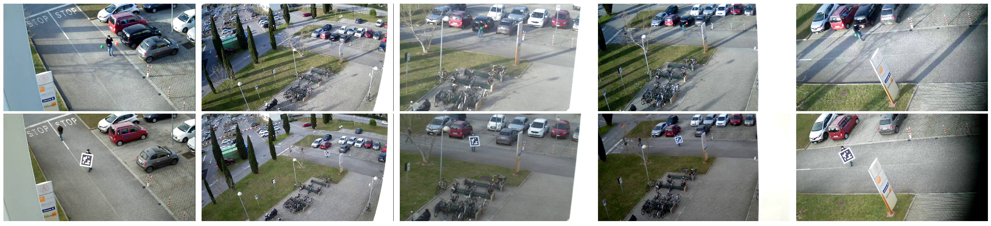
5.2. Outdoor Setup
6. Results
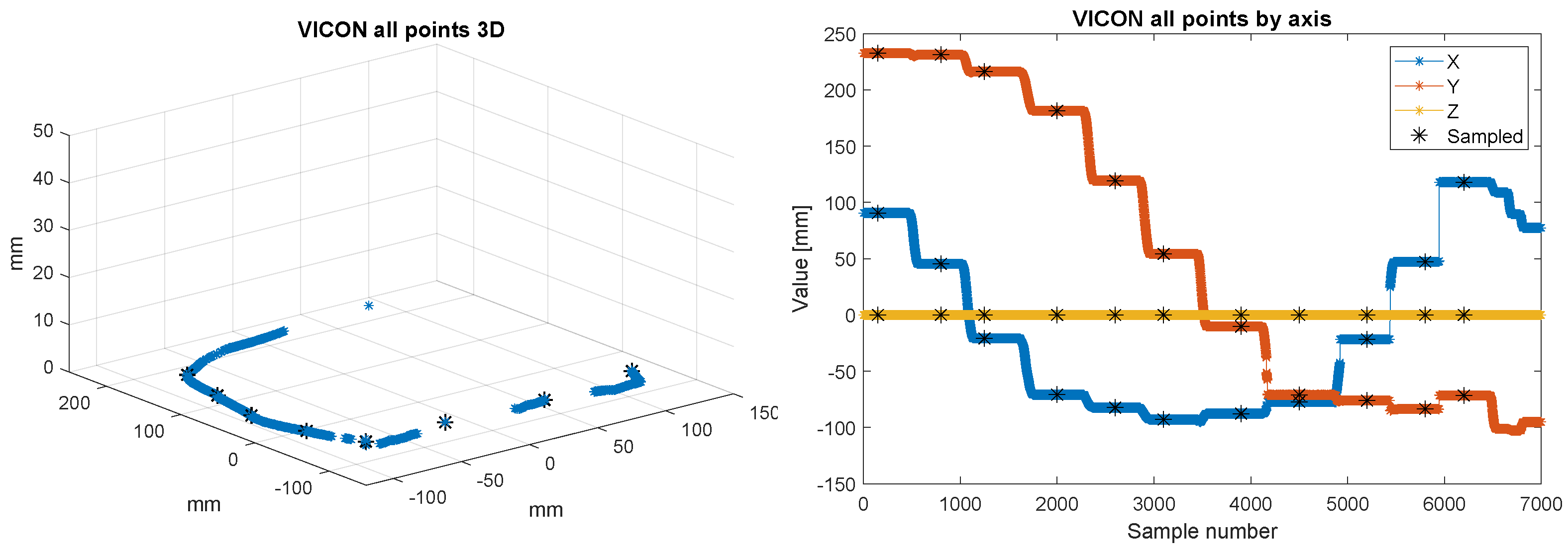
6.1. Ground Truth
6.2. Indoor Setup
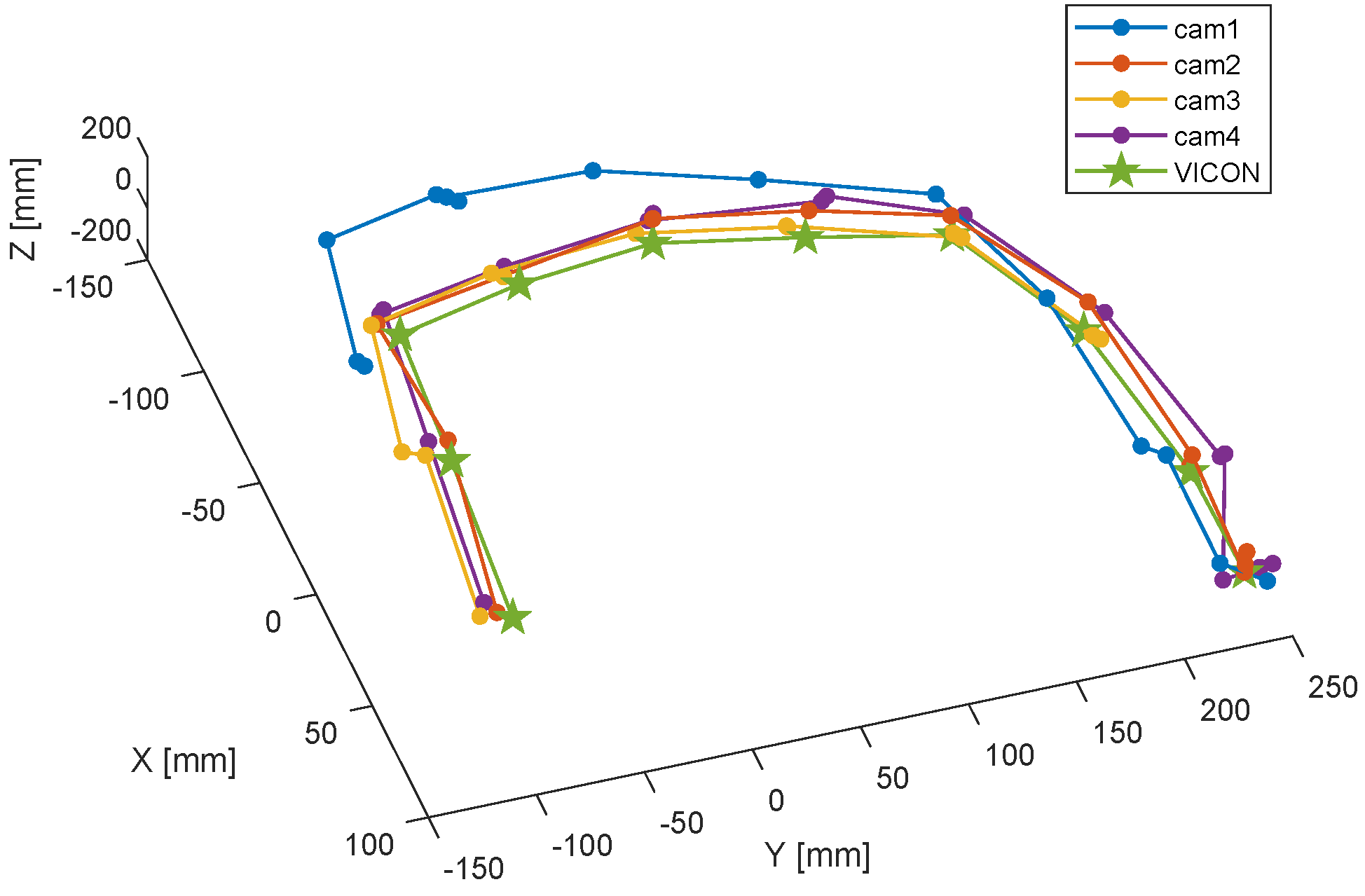
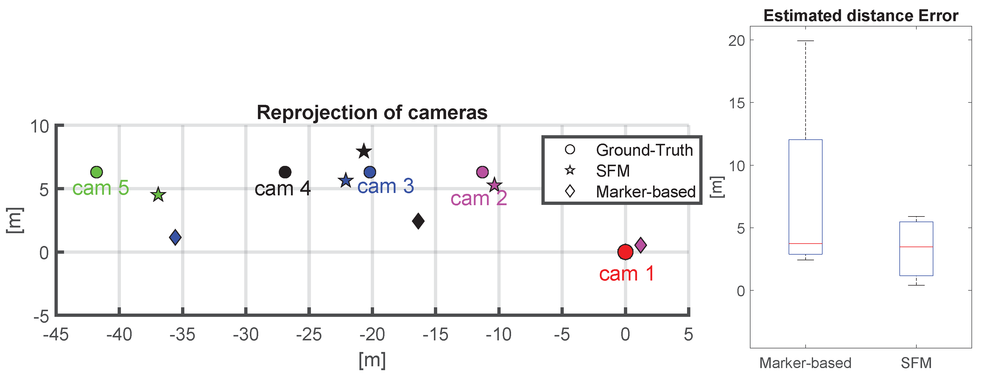
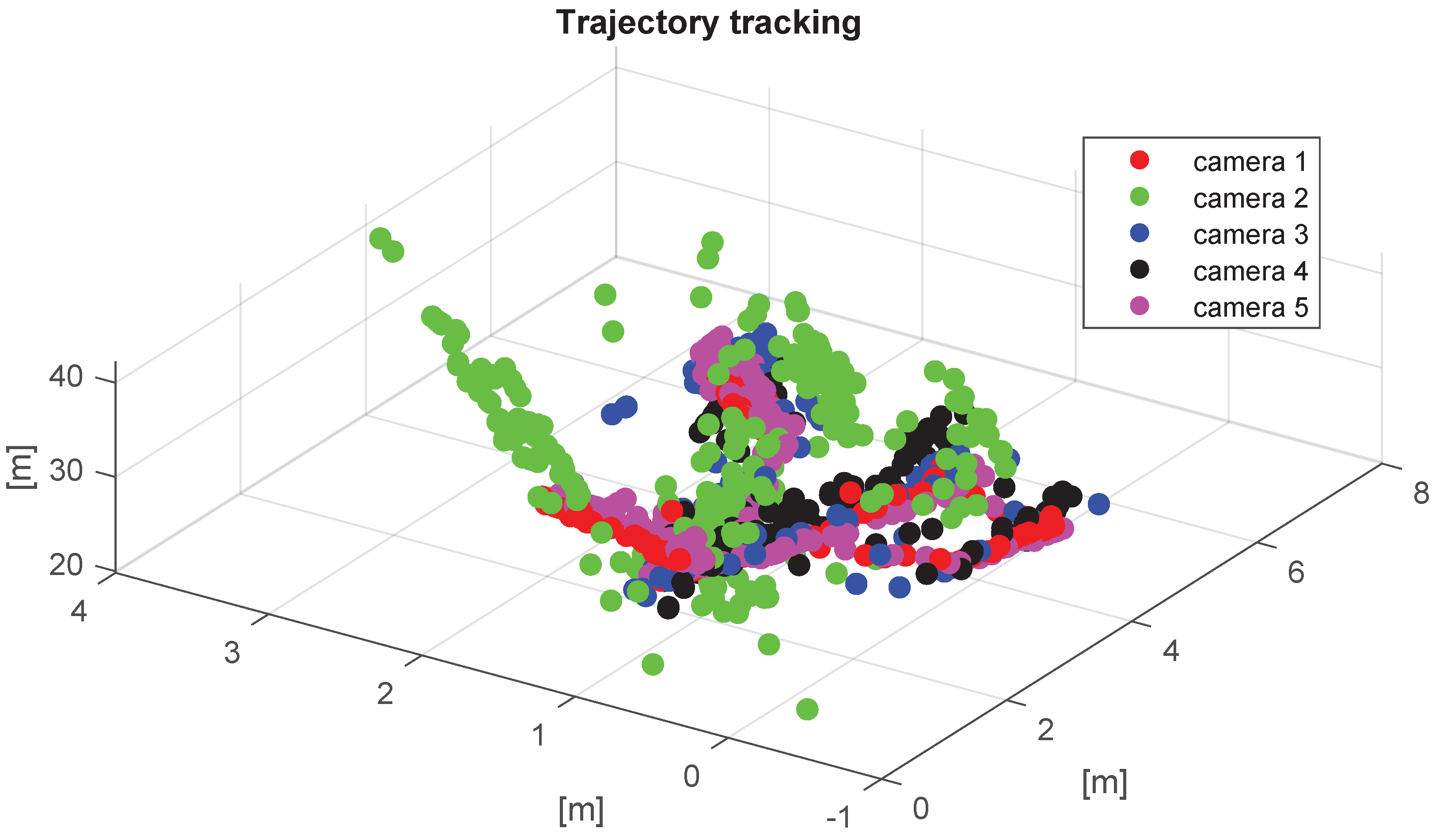
6.3. Outdoor Setup
7. Discussion
Limitations
8. Conclusions
Author Contributions
Funding
Institutional Review Board Statement
Informed Consent Statement
Data Availability Statement
Conflicts of Interest
References
- D’Avella, S.; Tripicchio, P.; Avizzano, C.A. A study on picking objects in cluttered environments: Exploiting depth features for a custom low-cost universal jamming gripper. Robot. Comput.-Integr. Manuf. 2020, 63, 101888. [Google Scholar] [CrossRef]
- Tripicchio, P.; Camacho-Gonzalez, G.; D’Avella, S. Welding defect detection: Coping with artifacts in the production line. Int. J. Adv. Manuf. Technol. 2020, 111, 1659–1669. [Google Scholar] [CrossRef]
- Filippeschi, A.; Pellicci, M.; Vanni, F.; Forte, G.; Bassani, G.; Landolfi, L.; De Merich, D.; Campo, G.; Avizzano, C.A.; Bergamasco, M. The Sailport Project: A Trilateral Approach to the Improvement of Workers’ Safety and Health in Ports. In Advances in Safety Management and Human Factors, Proceedings of the International Conference on Applied Human Factors and Ergonomics, Washington, DC, USA, 24–28 July 2019; Springer: Berlin/Heidelberg, Germany, 2019; pp. 69–80. [Google Scholar]
- Zhang, Z. Flexible camera calibration by viewing a plane from unknown orientations. In Proceedings of the Seventh IEEE International Conference on Computer Vision, Kerkyra, Greece, 20–27 September 1999; Volume 1, pp. 666–673. [Google Scholar]
- Luong, Q.T.; Faugeras, O.D. Self-calibration of a moving camera from point correspondences and fundamental matrices. Int. J. Comput. Vis. 1997, 22, 261–289. [Google Scholar] [CrossRef]
- Garrido-Jurado, S.; Muñoz Salinas, R.; Madrid-Cuevas, F.; Marín-Jiménez, M. Automatic Generation and Detection of Highly Reliable Fiducial Markers Under Occlusion. Pattern Recognit. 2014, 47, 2280–2292. [Google Scholar] [CrossRef]
- Olson, E. AprilTag: A robust and flexible visual fiducial system. In Proceedings of the 2011 IEEE International Conference on Robotics and Automation, Shanghai, China, 9–13 May 2011; pp. 3400–3407. [Google Scholar]
- Sagitov, A.; Shabalina, K.; Sabirova, L.; Li, H.; Magid, E. ARTag, AprilTag and CALTag Fiducial Marker Systems: Comparison in a Presence of Partial Marker Occlusion and Rotation. In Proceedings of the 14th International Conference on Informatics in Control, Automation and Robotics (ICINCO), Madrid, Spain, 26–28 July 2017; pp. 182–191. [Google Scholar] [CrossRef]
- Daftry, S.; Maurer, M.; Wendel, A.; Bischof, H. Flexible and User-Centric Camera Calibration using Planar Fiducial Markers. In Proceedings of the British Machine Vision Conference, Bristol, UK, 9–13 September 2013. [Google Scholar]
- Scaramuzza, D.; Fraundorfer, F. Visual odometry [tutorial]. IEEE Robot. Autom. Mag. 2011, 18, 80–92. [Google Scholar] [CrossRef]
- Yousif, K.; Bab-Hadiashar, A.; Hoseinnezhad, R. An Overview to Visual Odometry and Visual SLAM: Applications to Mobile Robotics. Intell. Ind. Syst. 2015, 1, 289–311. [Google Scholar] [CrossRef]
- Tripicchio, P.; Unetti, M.; Giordani, N.; Avizzano, C.A.; Satler, M. A lightweight slam algorithm for indoor autonomous navigation. In Proceedings of the Australasian Conference on Robotics and Automation (ACRA 2014), Melbourne, Australia, 2–4 December 2014. [Google Scholar]
- Hartley, R.I.; Zisserman, A. Multiple View Geometry in Computer Vision, 2nd ed.; Cambridge University Press: Cambridge, UK, 2004; ISBN 0521540518. [Google Scholar]
- Konolige, K.; Agrawal, M.; Solà, J. Large-Scale Visual Odometry for Rough Terrain. In Robotics Research: The 13th International Symposium ISRR; Kaneko, M., Nakamura, Y., Eds.; Springer: Berlin/Heidelberg, Germany, 2011; pp. 201–212. [Google Scholar] [CrossRef] [Green Version]
- Corke, P.; Strelow, D.; Singh, S. Omnidirectional visual odometry for a planetary rover. In Proceedings of the 2004 IEEE/RSJ International Conference on Intelligent Robots and Systems (IROS) (IEEE Cat. No.04CH37566), Sendai, Japan, 28 September–2 October 2004; Volume 4, pp. 4007–4012. [Google Scholar] [CrossRef] [Green Version]
- Forster, C.; Pizzoli, M.; Scaramuzza, D. SVO: Fast semi-direct monocular visual odometry. In Proceedings of the 2014 IEEE International Conference on Robotics and Automation (ICRA), Hong Kong, China, 31 May–7 June 2014; pp. 15–22. [Google Scholar]
- Yi, G.; Jianxin, L.; Hangping, Q.; Bo, W. Survey of structure from motion. In Proceedings of the 2014 International Conference on Cloud Computing and Internet of Things, Changchun, China, 13–14 December 2014; pp. 72–76. [Google Scholar] [CrossRef]
- Korthals, T.; Wolf, D.; Rudolph, D.; Hesse, M.; Rückert, U. Fiducial Marker based Extrinsic Camera Calibration for a Robot Benchmarking Platform. In Proceedings of the 2019 European Conference on Mobile Robots (ECMR), Prague, Czech Republic, 4–6 September 2019; pp. 1–6. [Google Scholar] [CrossRef]
- Harris, C.; Stephens, M. A combined corner and edge detector. In Proceedings of the Alvey Vision Conference, Manchester, UK, 31 August–2 September 1988; Volume 15, pp. 10–5244. [Google Scholar]
- Rosten, E.; Drummond, T. Machine learning for high-speed corner detection. In Proceedings of the European Conference on Computer Vision; Springer: Berlin/Heidelberg, Germany, 2006; pp. 430–443. [Google Scholar]
- Lowe, D.G. Distinctive image features from scale-invariant keypoints. Int. J. Comput. Vis. 2004, 60, 91–110. [Google Scholar] [CrossRef]
- Rublee, E.; Rabaud, V.; Konolige, K.; Bradski, G. ORB: An efficient alternative to SIFT or SURF. In Proceedings of the 2011 International Conference on Computer Vision, Barcelona, Spain, 6–13 November 2011; pp. 2564–2571. [Google Scholar]
- Jakubović, A.; Velagić, J. Image feature matching and object detection using brute-force matchers. In Proceedings of the 2018 International Symposium ELMAR, Zadar, Croatia, 16–19 September 2018; pp. 83–86. [Google Scholar]
- Muja, M.; Lowe, D. Flann-Fast Library for Approximate Nearest Neighbors User Manual; Computer Science Department, University of British Columbia: Vancouver, BC, Canada, 2009; Volume 5. [Google Scholar]
- DeTone, D.; Malisiewicz, T.; Rabinovich, A. Superpoint: Self-supervised interest point detection and description. In Proceedings of the IEEE Conference on Computer Vision and Pattern Recognition Workshops, Salt Lake City, UT, USA, 18–22 June 2018; pp. 224–236. [Google Scholar]
- Yang, T.Y.; Nguyen, D.K.; Heijnen, H.; Balntas, V. Ur2kid: Unifying retrieval, keypoint detection, and keypoint description without local correspondence supervision. arXiv 2020, arXiv:2001.07252. [Google Scholar]
- Dusmanu, M.; Rocco, I.; Pajdla, T.; Pollefeys, M.; Sivic, J.; Torii, A.; Sattler, T. D2-net: A trainable cnn for joint description and detection of local features. In Proceedings of the IEEE/CVF Conference on Computer Vision and Pattern Recognition, Long Beach, CA, USA, 15–20 June 2019; pp. 8092–8101. [Google Scholar]
- Li, H.; Hartley, R. Five-point motion estimation made easy. In Proceedings of the 18th International Conference on Pattern Recognition (ICPR’06), Hong Kong, China, 20–24 August 2006; Volume 1, pp. 630–633. [Google Scholar]
- Nistér, D. An efficient solution to the five-point relative pose problem. IEEE Trans. Pattern Anal. Mach. Intell. 2004, 26, 756–770. [Google Scholar] [CrossRef] [PubMed]
- Fischler, M.A.; Bolles, R.C. Random Sample Consensus: A Paradigm for Model Fitting with Applications to Image Analysis and Automated Cartography. Commun. ACM 1981, 24, 381–395. [Google Scholar] [CrossRef]
- Georgiev, G.H.; Radulov, V. A practical method for decomposition of the essential matrix. Appl. Math. Sci. 2014, 8, 8755–8770. [Google Scholar] [CrossRef]
- Triggs, B.; McLauchlan, P.F.; Hartley, R.I.; Fitzgibbon, A.W. Bundle adjustment—A modern synthesis. In Proceedings of the International Workshop on Vision Algorithms, Corfu, Greece, 21–22 September 1999; pp. 298–372. [Google Scholar]
- Balntas, V.; Li, S.; Prisacariu, V. Relocnet: Continuous metric learning relocalisation using neural nets. In Proceedings of the European Conference on Computer Vision (ECCV), Munich, Germany, 8–14 September 2018; pp. 751–767. [Google Scholar]
- Ding, M.; Wang, Z.; Sun, J.; Shi, J.; Luo, P. CamNet: Coarse-to-fine retrieval for camera re-localization. In Proceedings of the IEEE/CVF International Conference on Computer Vision, Seoul, Korea, 27 October–2 November 2019; pp. 2871–2880. [Google Scholar]
- Kendall, A.; Grimes, M.; Cipolla, R. Posenet: A convolutional network for real-time 6-dof camera relocalization. In Proceedings of the IEEE International Conference on Computer Vision, Santiago, Chile, 11–18 December 2015; pp. 2938–2946. [Google Scholar]
- Gu, J.; Wang, Z.; Kuen, J.; Ma, L.; Shahroudy, A.; Shuai, B.; Liu, T.; Wang, X.; Wang, G.; Cai, J.; et al. Recent advances in convolutional neural networks. Pattern Recognit. 2018, 77, 354–377. [Google Scholar] [CrossRef] [Green Version]
- Ullman, S. The interpretation of structure from motion. Proc. R. Soc. Lond. Ser. B Biol. Sci. 1979, 203, 405–426. [Google Scholar]
- Melekhov, I.; Ylioinas, J.; Kannala, J.; Rahtu, E. Relative camera pose estimation using convolutional neural networks. In Proceedings of the International Conference on Advanced Concepts for Intelligent Vision Systems, Auckland, New Zealand, 10–14 February 2017; pp. 675–687. [Google Scholar]
- Walch, F.; Hazirbas, C.; Leal-Taixe, L.; Sattler, T.; Hilsenbeck, S.; Cremers, D. Image-based localization using lstms for structured feature correlation. In Proceedings of the IEEE International Conference on Computer Vision, Venice, Italy, 22–29 October 2017; pp. 627–637. [Google Scholar]
- Kendall, A.; Cipolla, R. Geometric loss functions for camera pose regression with deep learning. In Proceedings of the IEEE Conference on Computer Vision and Pattern Recognition, Honolulu, HI, USA, 21–26 July 2017; pp. 5974–5983. [Google Scholar]
- Rocco, I.; Arandjelovic, R.; Sivic, J. Convolutional neural network architecture for geometric matching. In Proceedings of the IEEE Conference on Computer Vision and Pattern Recognition, Honolulu, HI, USA, 21–26 July 2017; pp. 6148–6157. [Google Scholar]
- Yi, K.M.; Trulls, E.; Ono, Y.; Lepetit, V.; Salzmann, M.; Fua, P. Learning to find good correspondences. In Proceedings of the IEEE Conference on Computer Vision and Pattern Recognition, Salt Lake City, UT, USA, 18–22 June 2018; pp. 2666–2674. [Google Scholar]
- Shavit, Y.; Ferens, R. Introduction to camera pose estimation with deep learning. arXiv 2019, arXiv:1907.05272. [Google Scholar]
- Xu, Y.; Li, Y.J.; Weng, X.; Kitani, K. Wide-Baseline Multi-Camera Calibration using Person Re-Identification. In Proceedings of the IEEE/CVF Conference on Computer Vision and Pattern Recognition, Nashville, TN, USA, 20–25 June 2021; pp. 13134–13143. [Google Scholar]
- Luong, Q.T.; Faugeras, O.D. The fundamental matrix: Theory, algorithms, and stability analysis. Int. J. Comput. Vis. 1996, 17, 43–75. [Google Scholar] [CrossRef]
- Nister, D. An efficient solution to the five-point relative pose problem. In Proceedings of the Computer Vision and Pattern Recognition, Madison, WI, USA, 16–22 June 2003; Volume 2, pp. 195–202. [Google Scholar] [CrossRef]
- Lourakis, M.L.A.; Argyros, A.A. Is Levenberg-Marquardt the most efficient optimization algorithm for implementing bundle adjustment? In Proceedings of the Tenth IEEE International Conference on Computer Vision (ICCV’05), Beijing, China, 17–21 October 2005; Volume 2, pp. 1526–1531. [Google Scholar] [CrossRef] [Green Version]
- Tsai, R. A versatile camera calibration technique for high-accuracy 3D machine vision metrology using off-the-shelf TV cameras and lenses. IEEE J. Robot. Autom. 1987, 3, 323–344. [Google Scholar] [CrossRef] [Green Version]
- Bazeille, S.; Filliat, D. Combining Odometry and Visual Loop-Closure Detection for Consistent Topo-Metrical Mapping. RAIRO—Oper. Res. 2011, 44, 365–377. [Google Scholar] [CrossRef] [Green Version]
- Fette, I.; Melnikov, A. The WebSocket Protocol. RFC 6455, RFC Editor. 2011. Available online: http://www.rfc-editor.org/rfc/rfc6455.txt (accessed on 12 June 2022).
- Dahl, R. Node. js: Evented I/O for v8 Javascript. Available online: https://www.nodejs.org (accessed on 12 June 2022).

| Name | Method | Features | N Cameras | Motion | Scalability |
|---|---|---|---|---|---|
| Korthals et al. [18] | Marker | Aruco | Multiple | Fixed | yes |
| based | indoor only | ||||
| RelocNet [33] | DNN | Frustum | 2 | Moving | yes |
| overlap | |||||
| CamNet [34] | DNN | Frustum | 2 | Moving | yes |
| overlap | |||||
| Yi et al. [42] | MLP | SIFT | 2 | Moving | yes |
| Xu et al. [44] | SfM | people | 2 | Fixed | no |
| bounding box | |||||
| This Paper | Marker | Aruco | Multiple | Fixed | yes |
| SfM | Wand |
| Type | Name |
|---|---|
| Computing node | Up Board with Intel(R) Atom(TM) x5-Z8350 |
| Camera | ELP-usbfhd04h-dl36 |
| Wifi dongle | ALFA AWUS036ACH |
| Wifi router | NETGEAR XR500 |
| Master node | Desktop with Intel(R) i7-5930K |
| Camera 1 | Camera 2 | Camera 3 | Camera 4 | Camera 5 | |
|---|---|---|---|---|---|
| Optics [mm] | 8 | 8 | 12 | 6 | 3.6 |
Publisher’s Note: MDPI stays neutral with regard to jurisdictional claims in published maps and institutional affiliations. |
© 2022 by the authors. Licensee MDPI, Basel, Switzerland. This article is an open access article distributed under the terms and conditions of the Creative Commons Attribution (CC BY) license (https://creativecommons.org/licenses/by/4.0/).
Share and Cite
Tripicchio, P.; D’Avella, S.; Camacho-Gonzalez, G.; Landolfi, L.; Baris, G.; Avizzano, C.A.; Filippeschi, A. Multi-Camera Extrinsic Calibration for Real-Time Tracking in Large Outdoor Environments. J. Sens. Actuator Netw. 2022, 11, 40. https://doi.org/10.3390/jsan11030040
Tripicchio P, D’Avella S, Camacho-Gonzalez G, Landolfi L, Baris G, Avizzano CA, Filippeschi A. Multi-Camera Extrinsic Calibration for Real-Time Tracking in Large Outdoor Environments. Journal of Sensor and Actuator Networks. 2022; 11(3):40. https://doi.org/10.3390/jsan11030040
Chicago/Turabian StyleTripicchio, Paolo, Salvatore D’Avella, Gerardo Camacho-Gonzalez, Lorenzo Landolfi, Gabriele Baris, Carlo Alberto Avizzano, and Alessandro Filippeschi. 2022. "Multi-Camera Extrinsic Calibration for Real-Time Tracking in Large Outdoor Environments" Journal of Sensor and Actuator Networks 11, no. 3: 40. https://doi.org/10.3390/jsan11030040
APA StyleTripicchio, P., D’Avella, S., Camacho-Gonzalez, G., Landolfi, L., Baris, G., Avizzano, C. A., & Filippeschi, A. (2022). Multi-Camera Extrinsic Calibration for Real-Time Tracking in Large Outdoor Environments. Journal of Sensor and Actuator Networks, 11(3), 40. https://doi.org/10.3390/jsan11030040