Impact of Image Compression on the Performance of Steel Surface Defect Classification with a CNN

 ,
, 
Abstract
:1. Introduction
- Identifying the parameters that can be used to compress images as much as possible, without losing the accuracy of classification with a CNN;
- Evaluating the impact of image compression on the classification performance of a CNN that is trained and tested using compressed image datasets with the same parameters;
- Investigating the impact of image compression on the classification performance of a trained and tested CNN using compressed image datasets with different parameters;
- Studying the benefit of compression-based data augmentation on the classification performance of a CNN.
2. Related Work
3. Theoretical Background
4. Methodology
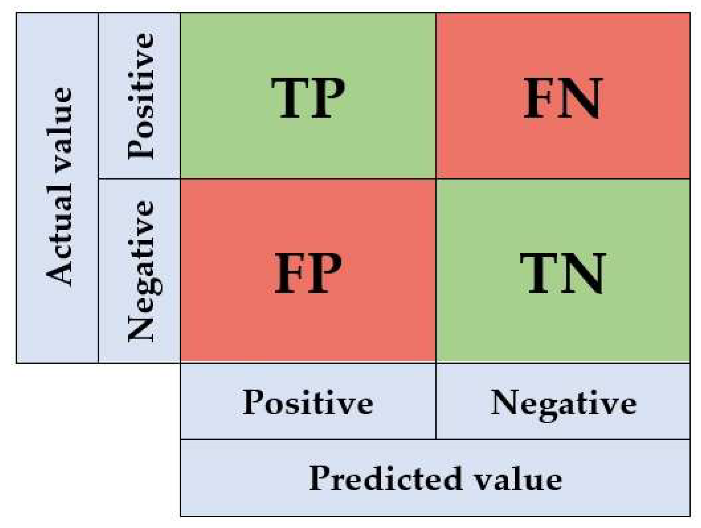
- True Positive (TP): predicted a positive class as positive;
- False Positive (FP): predicted a negative class as positive;
- False Negative (FN): predicted a positive class as negative;
- True Negative (TN): predicted a negative class as negative.
- is the average of x and is the average of y;
- is the variance of x and is the variance of y;
- is the covariance of x and y;
- and are two variables to stabilize the division with a weak denominator;
- L is the dynamic range of the pixel values (typically, this is );
- k1 = 0.01 and k2 = 0.03 by default.
5. Results and Discussion
6. Conclusions
Author Contributions
Funding
Institutional Review Board Statement
Informed Consent Statement
Data Availability Statement
Conflicts of Interest
References
- Ghobakhloo, M.; Fathi, M.; Iranmanesh, M.; Maroufkhani, P.; Morales, M.E. Industry 4.0 ten years on: A bibliometric and systematic review of concepts, sustainability value drivers, and success determinants. J. Clean. Prod. 2021, 302, 127052. [Google Scholar] [CrossRef]
- Bousdekis, A.; Lepenioti, K.; Apostolou, D.; Mentzas, G. A Review of Data-Driven Decision-Making Methods for Industry 4.0 Maintenance Applications. Electronics 2021, 10, 828. [Google Scholar] [CrossRef]
- Elsisi, M.; Mahmoud, K.; Lehtonen, M.; Darwish, M.M.F. Reliable Industry 4.0 Based on Machine Learning and IoT for Analyzing, Monitoring, and Securing Smart Meters. Sensors 2021, 21, 487. [Google Scholar] [CrossRef]
- Khairnar, V.; Kolhe, L.; Bhagat, S.; Sahu, R.; Kumar, A.; Shaikh, S. Industrial Automation of Process for Transformer Monitoring System Using IoT Analytics. In Inventive Communication and Computational Technologies; Springer: Singapore, 2020; pp. 1191–1200. [Google Scholar] [CrossRef]
- Theissler, A.; Pérez-Velázquez, J.; Kettelgerdes, M.; Elger, G. Predictive maintenance enabled by machine learning: Use cases and challenges in the automotive industry. Reliab. Eng. Syst. Saf. 2021, 215, 107864. [Google Scholar] [CrossRef]
- Devasthali, A.S.; Chaudhari, A.J.; Bhutada, S.S.; Doshi, S.R.; Suryawanshi, V.P. IoT Based Inventory Management System with Recipe Recommendation Using Collaborative Filtering. In Evolutionary Computing and Mobile Sustainable Networks; Springer: Singapore, 2020; pp. 543–550. [Google Scholar] [CrossRef]
- Shahbazi, Z.; Byun, Y.-C. Integration of Blockchain, IoT and Machine Learning for Multistage Quality Control and Enhancing Security in Smart Manufacturing. Sensors 2021, 21, 1467. [Google Scholar] [CrossRef]
- Silva, R.L.; Junior, O.C.; Rudek, M. A road map for planning-deploying machine vision artifacts in the context of industry 4.0. J. Ind. Prod. Eng. 2021, 1–14. [Google Scholar] [CrossRef]
- Banda, T.; Jie, B.Y.W.; Farid, A.A.; Lim, C.S. Machine Vision and Convolutional Neural Networks for Tool Wear Identification and Classification. In Recent Trends in Mechatronics Towards Industry 4.0; Springer: Singapore, 2021; pp. 737–747. [Google Scholar] [CrossRef]
- Pundir, M.; Sandhu, J.K. A Systematic Review of Quality of Service in Wireless Sensor Networks using Machine Learning: Recent Trend and Future Vision. J. Netw. Comput. Appl. 2021, 188, 103084. [Google Scholar] [CrossRef]
- Benbarrad, T.; Salhaoui, M.; Kenitar, S.; Arioua, M. Intelligent Machine Vision Model for Defective Product Inspection Based on Machine Learning. J. Sens. Actuator Netw. 2021, 10, 7. [Google Scholar] [CrossRef]
- Luo, Y.; Li, S.; Li, D. Intelligent Perception System of Robot Visual Servo for Complex Industrial Environment. Sensors 2020, 20, 7121. [Google Scholar] [CrossRef] [PubMed]
- Mou, H.R.; Lu, R.; An, J. Research on Machine Vision Technology of High Speed Robot Sorting System based on Deep Learning. J. Physics Conf. Ser. 2021, 1748, 022029. [Google Scholar] [CrossRef]
- Luo, Q.; Fang, X.; Su, J.; Zhou, J.; Zhou, B.; Yang, C.; Liu, L.; Gui, W.; Tian, L. Automated Visual Defect Classification for Flat Steel Surface: A Survey. IEEE Trans. Instrum. Meas. 2020, 69, 9329–9349. [Google Scholar] [CrossRef]
- Chu, M.-X.; Feng, Y.; Yang, Y.-H.; Deng, X. Multi-class classification method for steel surface defects with feature noise. J. Iron Steel Res. Int. 2020, 28, 303–315. [Google Scholar] [CrossRef]
- Wang, S.; Xia, X.; Ye, L.; Yang, B. Automatic Detection and Classification of Steel Surface Defect Using Deep Convolutional Neural Networks. Metals 2021, 11, 388. [Google Scholar] [CrossRef]
- Konovalenko, I.; Maruschak, P.; Brezinová, J.; Viňáš, J.; Brezina, J. Steel Surface Defect Classification Using Deep Residual Neural Network. Metals 2020, 10, 846. [Google Scholar] [CrossRef]
- Benbarrad, T.; Salhaoui, M.; Arioua, M. On the Performance of Deep Learning in the Full Edge and the Full Cloud Architectures. In Proceedings of the 4th International Conference on Networking, Information Systems & Security, New York, NY, USA, 1–4 April 2021. [Google Scholar] [CrossRef]
- Bouakkaz, F.; Ali, W.; Derdour, M. Forest Fire Detection Using Wireless Multimedia Sensor Networks and Image Compression. Instrum. Mes. Métrologie 2021, 20, 57–63. [Google Scholar] [CrossRef]
- Hussain, A.J.; Al-Fayadh, A.; Radi, N. Image compression techniques: A survey in lossless and lossy algorithms. Neurocomputing 2018, 300, 44–69. [Google Scholar] [CrossRef]
- Song, K.; Yan, Y. A noise robust method based on completed local binary patterns for hot-rolled steel strip surface defects. Appl. Surf. Sci. 2013, 285, 858–864. [Google Scholar] [CrossRef]
- Jo, Y.-Y.; Choi, Y.S.; Park, H.W.; Lee, J.H.; Jung, H.; Kim, H.-E.; Ko, K.; Lee, C.W.; Cha, H.S.; Hwangbo, Y. Impact of image compression on deep learning-based mammogram classification. Sci. Rep. 2021, 11, 7924. [Google Scholar] [CrossRef]
- Bouderbal, I.; Amamra, A.; Benatia, M.A. How Would Image Down-Sampling and Compression Impact Object Detection in the Context of Self-driving Vehicles. In Advances in Computing Systems and Applications; Springer: Cham, Switzerland, 2021; pp. 25–37. [Google Scholar] [CrossRef]
- Poyser, M.; Atapour-Abarghouei, A.; Breckon, T.P. On the Impact of Lossy Image and Video Compression on the Performance of Deep Convolutional Neural Network Architectures. In Proceedings of the 2020 25th International Conference on Pattern Recognition (ICPR), Milan, Italy, 10–15 January 2021; pp. 2830–2837. [Google Scholar] [CrossRef]
- Steffens, C.R.; Messias, L.R.V.; Drews, P., Jr.; Botelho, S.S.D.C. Can Exposure, Noise and Compression Affect Image Recognition? An Assessment of the Impacts on State-of-the-Art ConvNets. In Proceedings of the 2019 Latin American Robotics Symposium (LARS), 2019 Brazilian Symposium on Robotics (SBR) and 2019 Workshop on Robotics in Education (WRE), Rio Grande, Brazil, 23–25 October 2019; pp. 61–66. [Google Scholar] [CrossRef]
- Zanjani, F.G.; Zinger, S.; Piepers, B.; Mahmoudpour, S.; Schelkens, P. Impact of JPEG 2000 compression on deep convolutional neural networks for metastatic cancer detection in histopathological images. J. Med. Imaging 2019, 6, 027501. [Google Scholar] [CrossRef]
- Aydin, I.; Akin, E.; Karakose, M. Defect classification based on deep features for railway tracks in sustainable transportation. Appl. Soft Comput. 2021, 111, 107706. [Google Scholar] [CrossRef]
- Chen, K.; Zeng, Z.; Yang, J. A deep region-based pyramid neural network for automatic detection and multi-classification of various surface defects of aluminum alloys. J. Build. Eng. 2021, 43, 102523. [Google Scholar] [CrossRef]
- He, Y.; Song, K.; Meng, Q.; Yan, Y. An End-to-End Steel Surface Defect Detection Approach via Fusing Multiple Hierarchical Features. IEEE Trans. Instrum. Meas. 2019, 69, 1493–1504. [Google Scholar] [CrossRef]
- Abu, M.; Amir, A.; Lean, Y.H.; Zahri, N.A.H.; Azemi, S.A. The Performance Analysis of Transfer Learning for Steel Defect Detection by Using Deep Learning. J. Phys. Conf. Ser. 2021, 1755. [Google Scholar] [CrossRef]
- Zhang, J.; Li, Z.; Hao, R.; Wang, X.; Du, X.; Yan, B.; Ni, G.; Liu, J.; Liu, L.; Liu, Y. Classification of Microscopic Laser Engraving Surface Defect Images Based on Transfer Learning Method. Electronics 2021, 10, 1993. [Google Scholar] [CrossRef]
- Wan, X.; Zhang, X.; Liu, L. An Improved VGG19 Transfer Learning Strip Steel Surface Defect Recognition Deep Neural Network Based on Few Samples and Imbalanced Datasets. Appl. Sci. 2021, 11, 2606. [Google Scholar] [CrossRef]
- Konovalenko, I.; Maruschak, P.; Brevus, V.; Prentkovskis, O. Recognition of Scratches and Abrasions on Metal Surfaces Using a Classifier Based on a Convolutional Neural Network. Metals 2021, 11, 549. [Google Scholar] [CrossRef]
- Fu, P.; Hu, B.; Lan, X.; Yu, J.; Ye, J. Simulation and quantitative study of cracks in 304 stainless steel under natural magnetization field. NDT E Int. 2021, 119, 102419. [Google Scholar] [CrossRef]
- Alzubaidi, L.; Zhang, J.; Humaidi, A.J.; Al-Dujaili, A.; Duan, Y.; Al-Shamma, O.; Santamaría, J.; Fadhel, M.A.; Al-Amidie, M.; Farhan, L. Review of deep learning: Concepts, CNN architectures, challenges, applications, future directions. J. Big Data 2021, 8, 53. [Google Scholar] [CrossRef]
- Yeganeh, A.; Pourpanah, F.; Shadman, A. An ANN-based ensemble model for change point estimation in control charts. Appl. Soft Comput. 2021, 110, 107604. [Google Scholar] [CrossRef]
- Chai, Q. Research on the Application of Computer CNN in Image Recognition. J. Phys. Conf. Ser. 2021, 1915, 032041. [Google Scholar] [CrossRef]
- Ban, H.; Ning, J. Design of English Automatic Translation System Based on Machine Intelligent Translation and Secure Internet of Things. Mob. Inf. Syst. 2021, 2021, 8670739. [Google Scholar] [CrossRef]
- Muhammad, K.; Ullah, A.; Lloret, J.; Del Ser, J.; de Albuquerque, V.H.C. Deep Learning for Safe Autonomous Driving: Current Challenges and Future Directions. IEEE Trans. Intell. Transp. Syst. 2020, 22, 4316–4336. [Google Scholar] [CrossRef]
- Meng, L.; Yuesong, W.; Jinqi, L. Design of an Intelligent Service Robot based on Deep Learning. In Proceedings of the ICIT 2020: 2020 The 8th International Conference on Information Technology: IoT and Smart City, Xi’an, China, 25–27 December 2020. [Google Scholar] [CrossRef]
- Yu, T.; Jin, H.; Tan, W.-T.; Nahrstedt, K. SKEPRID. ACM Trans. Multimed. Comput. Commun. Appl. 2018, 14, 1–24. [Google Scholar] [CrossRef]
- Yang, Q.; Li, C.; Dai, W.; Zou, J.; Qi, G.-J.; Xiong, H. Rotation Equivariant Graph Convolutional Network for Spherical Image Classification. In Proceedings of the IEEE/CVF Conference on Computer Vision and Pattern Recognition (CVPR), Seattle, WA, USA, 13–19 June 2020; pp. 4302–4311. [Google Scholar] [CrossRef]
- Ling, J.; Xue, H.; Song, L.; Xie, R.; Gu, X. Region-aware Adaptive Instance Normalization for Image Harmonization. In Proceedings of the IEEE/CVF Conference on Computer Vision and Pattern Recognition (CVPR), Nashville, TN, USA, 20–25 June 2021; pp. 9357–9366. [Google Scholar] [CrossRef]
- Pavlova, M.T. A Comparison of the Accuracies of a Convolution Neural Network Built on Different Types of Convolution Layers. In Proceedings of the 2021 56th International Scientific Conference on Information, Communication and Energy Systems and Technologies (ICEST), Sozopol, Bulgaria, 16–18 June 2021; pp. 81–84. [Google Scholar] [CrossRef]
- El Jaafari, I.; Ellahyani, A.; Charfi, S. Rectified non-linear unit for convolution neural network. J. Phys. Conf. Ser. 2021, 1743, 012014. [Google Scholar] [CrossRef]
- Wu, L.; Perin, G. On the Importance of Pooling Layer Tuning for Profiling Side-Channel Analysis. In Applied Cryptography and Network Security Workshops; Springer: Cham, Switzerland, 2021; pp. 114–132. [Google Scholar] [CrossRef]
- Matsumura, N.; Ito, Y.; Nakano, K.; Kasagi, A.; Tabaru, T. A novel structured sparse fully connected layer in convolutional neural networks. Concurr. Comput. Pract. Exp. 2021, e6213. [Google Scholar] [CrossRef]
- Semenov, A.; Boginski, V.; Pasiliao, E.L. Neural Networks with Multidimensional Cross-Entropy Loss Functions. In Computational Data and Social Networks; Springer: Cham, Switzerland, 2019; pp. 57–62. [Google Scholar] [CrossRef]
- Jayasankar, U.; Thirumal, V.; Ponnurangam, D. A survey on data compression techniques: From the perspective of data quality, coding schemes, data type and applications. J. King Saud Univ. Comput. Inf. Sci. 2021, 33, 119–140. [Google Scholar] [CrossRef]
- Qasim, A.J.; Din, R.; Alyousuf, F.Q.A. Review on techniques and file formats of image compression. Bull. Electr. Eng. Inform. 2020, 9, 602–610. [Google Scholar] [CrossRef]
- Iqbal, Y.; Kwon, O.-J. Improved JPEG Coding by Filtering 8 × 8 DCT Blocks. J. Imaging 2021, 7, 117. [Google Scholar] [CrossRef]
- Xiao, W.; Wan, N.; Hong, A.; Chen, X. A Fast JPEG Image Compression Algorithm Based on DCT. In Proceedings of the 2020 IEEE International Conference on Smart Cloud (SmartCloud), Washington, DC, USA, 6–8 November 2020; pp. 106–110. [Google Scholar] [CrossRef]
- Araujo, L.C.; Sansao, J.P.H.; Junior, M.C.S. Effects of Color Quantization on JPEG Compression. Int. J. Image Graph. 2020, 20, 2050026. [Google Scholar] [CrossRef]
- Bharadwaj, N.A.; Rao, C.S.; Rahul; Gururaj, C. Optimized Data Compression through Effective Analysis of JPEG Standard. In Proceedings of the 2021 International Conference on Emerging Smart Computing and Informatics (ESCI), Pune, India, 5–7 March 2021; pp. 110–115. [Google Scholar] [CrossRef]
- Ghaffari, A. Image compression-encryption method based on two-dimensional sparse recovery and chaotic system. Sci. Rep. 2021, 11, 1–19. [Google Scholar] [CrossRef]
- Simonyan, K.; Zisserman, A. Very Deep Convolutional Networks for Large-Scale Image Recognition. arXiv 2014, arXiv:1409.1556. Available online: https://arxiv.org/abs/1409.1556 (accessed on 6 August 2021).
- Howard, A.G.; Zhu, M.; Chen, B.; Kalenichenko, D.; Wang, W.; Weyand, T.; Andreetto, M.; Adam, H. MobileNets: Efficient Convolutional Neural Networks for Mobile Vision Applications. arXiv 2017, arXiv:1704.04861. Available online: http://arxiv.org/abs/1704.04861 (accessed on 10 August 2021).
- Kingma, D.; Ba, J. Adam: A Method for Stochastic Optimization. arXiv 2014, arXiv:1412.6980. Available online: https://arxiv.org/abs/1412.6980 (accessed on 8 August 2021).
- Choi, H.R.; Kang, S.-H.; Lee, S.; Han, D.-K.; Lee, Y. Comparison of image performance for three compression methods based on digital X-ray system: Phantom study. Optik 2018, 157, 197–202. [Google Scholar] [CrossRef]
- Wang, Z.; Bovik, A.C.; Sheikh, H.R.; Simoncelli, E.P. Image Quality Assessment: From Error Visibility to Structural Similarity. IEEE Trans. Image Process. 2004, 13, 600–612. [Google Scholar] [CrossRef] [Green Version]


| Designation | Compression Parameters | CR | |
|---|---|---|---|
| Scale | Quality | ||
| Q1 | 1/1 | 5 | 27.32 |
| Q2 | 1/1 | 10 | 21.69 |
| Q3 | 1/1 | 20 | 15.46 |
| Q4 | 1/1 | 30 | 12.41 |
| Q5 | 1/1 | 40 | 10.63 |
| Q6 | 1/1 | 50 | 9.33 |
| Q7 | 1/1 | 60 | 8.21 |
| Model/Data | Q1 | Q2 | Q3 | Q4 | Q5 | Q6 | Q7 |
|---|---|---|---|---|---|---|---|
| CNN3 | (0.85, 0.83, 0.82) | (0.89, 0.87, 0.87) | (0.88, 0.86, 0.86) | (0.84, 0.81, 0.80) | (0.89, 0.88, 0.87) | (0.83, 0.81, 0.81) | (0.86, 0.82, 0.82) |
| MobileNet | (0.97, 0.97, 0.97) | (0.99, 0.99, 0.99) | (0.98, 0.98, 0.98) | (0.98, 0.98, 0.98) | (0.98, 0.98, 0.98) | (0.98, 0.98, 0.98) | (1.00, 1.00, 1.00) |
| Vgg16 | (0.92, 0.91, 0.91) | (0.92, 0.91, 0.91) | (0.94, 0.93, 0.92) | (0.94, 0.93, 0.93) | (0.90, 0.90, 0.90) | (0.93, 0.92, 0.91) | (0.92, 0.90, 0.90) |
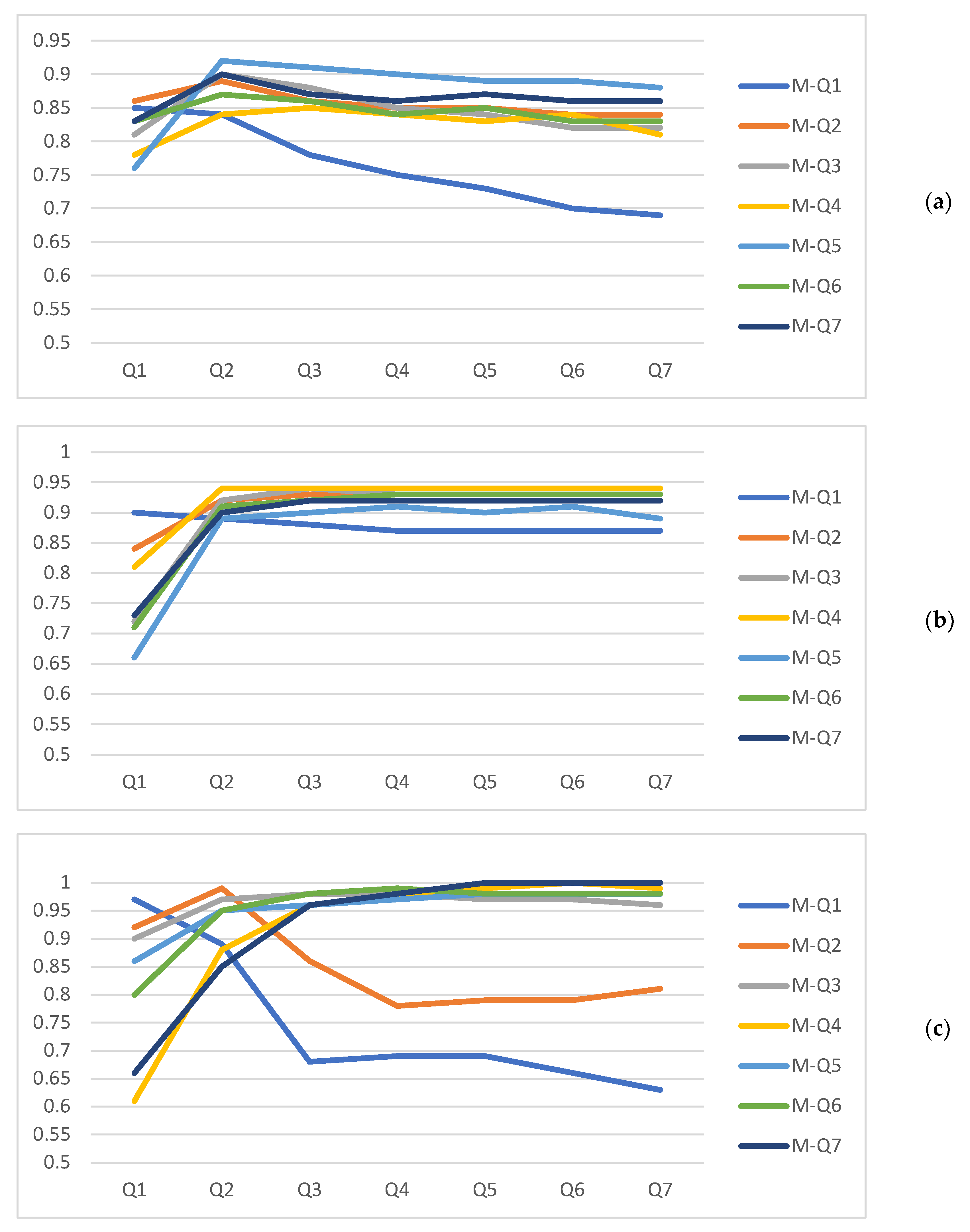
| Model/Data | Q1 | Q2 | Q3 | Q4 | Q5 | Q6 | Q7 |
|---|---|---|---|---|---|---|---|
| CNN3 | |||||||
| M-Q1 | (0.85, 0.83, 0.82) | (0.84, 0.81, 0.81) | (0.78, 0.74, 0.72) | (0.75, 0.71, 0.69) | (0.73, 0.71, 0.68) | (0.70, 0.69, 0.66) | (0.69, 0.69, 0.66) |
| M-Q2 | (0.86, 0.84, 0.84) | (0.89, 0.87, 0.87) | (0.86, 0.84, 0.83) | (0.85, 0.81, 0.81) | (0.85, 0.81, 0.80) | (0.84, 0.81, 0.81) | (0.84, 0.79, 0.79) |
| M-Q3 | (0.81, 0.67, 0.63) | (0.90, 0.89, 0.88) | (0.88, 0.86, 0.86) | (0.85, 0.83, 0.82) | (0.84, 0.81, 0.81) | (0.82, 0.78, 0.78) | (0.82, 0.78, 0.77) |
| M-Q4 | (0.78, 0.73, 0.68) | (0.84, 0.79, 0.78) | (0.85, 0.81, 0.81) | (0.84, 0.81, 0.80) | (0.83, 0.79, 0.79) | (0.84, 0.78, 0.78) | (0.81, 0.76, 0.76) |
| M-Q5 | (0.76, 0.67, 0.66) | (0.92, 0.91, 0.91) | (0.91, 0.90, 0.90) | (0.90, 0.88, 0.88) | (0.89, 0.88, 0.87) | (0.89, 0.88, 0.87) | (0.88, 0.86, 0.86) |
| M-Q6 | (0.83, 0.81, 0.80) | (0.87, 0.86, 0.85) | (0.86, 0.84, 0.84) | (0.84, 0.83, 0.83) | (0.85, 0.83, 0.83) | (0.83, 0.81, 0.81) | (0.83, 0.81, 0.81) |
| M-Q7 | (0.83, 0.81, 0.80) | (0.90, 0.87, 0.87) | (0.87, 0.85, 0.85) | (0.86, 0.83, 0.83) | (0.87, 0.84, 0.84) | (0.86, 0.83, 0.83) | (0.86, 0.82, 0.82) |
| MobileNet | |||||||
| M-Q1 | (0.97, 0.97, 0.97) | (0.89, 0.82, 0.79) | (0.68, 0.73, 0.67) | (0.69, 0.76, 0.70) | (0.69, 0.76, 0.71) | (0.66, 0.56, 0.49) | (0.63, 0.56, 0.44) |
| M-Q2 | (0.92, 0.90, 0.90) | (0.99, 0.99, 0.99) | (0.86, 0.83, 0.81) | (0.78, 0.75, 0.71) | (0.79, 0.75, 0.71) | (0.79, 0.75, 0.70) | (0.81, 0.76, 0.71) |
| M-Q3 | (0.90, 0.88, 0.89) | (0.97, 0.96, 0.96) | (0.98, 0.98, 0.98) | (0.98, 0.97, 0.98) | (0.97, 0.96, 0.96) | (0.97, 0.97, 0.97) | (0.96, 0.96, 0.96) |
| M-Q4 | (0.61, 0.23, 0.15) | (0.88, 0.81, 0.79) | (0.96, 0.96, 0.96) | (0.98, 0.98, 0.98) | (0.99, 0.99, 0.99) | (1.00, 1.00, 1.00) | (0.99, 0.99, 0.99) |
| M-Q5 | (0.86, 0.84, 0.83) | (0.95, 0.94, 0.93) | (0.96, 0.95, 0.95) | (0.97, 0.97, 0.96) | (0.98, 0.98, 0.98) | (0.98, 0.98, 0.98) | (0.98, 0.98, 0.98) |
| M-Q6 | (0.80, 0.74, 0.72) | (0.95, 0.95, 0.95) | (0.98, 0.98, 0.98) | (0.99, 0.99, 0.99) | (0.98, 0.98, 0.98) | (0.98, 0.98, 0.98) | (0.98, 0.98, 0.98) |
| M-Q7 | (0.66, 0.56, 0.49) | (0.85, 0.83, 0.83) | (0.96, 0.95, 0.95) | (0.98, 0.98, 0.98) | (1.00, 1.00, 1.00) | (1.00, 1.00, 1.00) | (1.00, 1.00, 1.00) |
| Vgg16 | |||||||
| M-Q1 | (0.90, 0.88, 0.88) | (0.89, 0.86, 0.86) | (0.88, 0.84, 0.84) | (0.87, 0.83, 0.83) | (0.87, 0.83, 0.83) | (0.87, 0.82, 0.82) | (0.87, 0.82, 0.82) |
| M-Q2 | (0.84, 0.83, 0.82) | (0.92, 0.91, 0.91) | (0.93, 0.92, 0.92) | (0.93, 0.92, 0.92) | (0.93, 0.92, 0.92) | (0.93, 0.91, 0.91) | (0.93, 0.91, 0.91) |
| M-Q3 | (0.72, 0.66, 0.62) | (0.92, 0.91, 0.91) | (0.94, 0.93, 0.92) | (0.93, 0.92, 0.92) | (0.93, 0.92, 0.91) | (0.93, 0.92, 0.91) | (0.93, 0.92, 0.91) |
| M-Q4 | (0.81, 0.79, 0.78) | (0.94, 0.93, 0.93) | (0.94, 0.93, 0.93) | (0.94, 0.93, 0.93) | (0.94, 0.93, 0.93) | (0.94, 0.93, 0.93) | (0.94, 0.93, 0.93) |
| M-Q5 | (0.66, 0.57, 0.54) | (0.89, 0.88, 0.88) | (0.90, 0.90, 0.90) | (0.91, 0.91, 0.91) | (0.90, 0.90, 0.90) | (0.91, 0.91, 0.90) | (0.89, 0.88, 0.88) |
| M-Q6 | (0.71, 0.66, 0.63) | (0.91, 0.90, 0.90) | (0.92, 0.91, 0.91) | (0.93, 0.92, 0.92) | (0.93, 0.92, 0.92) | (0.93, 0.92, 0.91) | (0.93, 0.91, 0.91) |
| M-Q7 | (0.73, 0.62, 0.58) | (0.90, 0.89, 0.89) | (0.92, 0.90, 0.90) | (0.92, 0.89, 0.89) | (0.92, 0.89, 0.88) | (0.92, 0.90, 0.89) | (0.92, 0.90, 0.90) |
| Q1 | Q2 | Q3 | Q4 | Q5 | Q6 | Q7 | |
|---|---|---|---|---|---|---|---|
| Q1 | 27.88/0.7073 | 28.23/0.6950 | 28.27/0.6887 | 28.23/0.6830 | 28.19/0.6784 | 28.16/0.6742 | |
| Q2 | 27.88/0.7073 | 31.04/0.7876 | 31.82/0.8081 | 31.24/0.7816 | 31.48/0.7879 | 31.16/0.7733 | |
| Q3 | 28.23/0.6950 | 31.04/0.7876 | 34.49/0.8848 | 33.72/0.8593 | 33.91/0.8611 | 34.12/0.8666 | |
| Q4 | 28.27/0.6887 | 31.82/0.8081 | 34.49/0.8848 | 36.59/0.9260 | 35.53/0.9007 | 35.01/0.8864 | |
| Q5 | 28.23/0.6830 | 31.24/0.7816 | 33.72/0.8593 | 36.59/0.9260 | 37.84/0.9429 | 36.42/0.9167 | |
| Q6 | 28.19/0.6784 | 31.48/0.7879 | 33.91/0.8611 | 35.53/0.9007 | 37.84/0.9429 | 38.55/0.9497 | |
| Q7 | 28.16/0.6742 | 31.16/0.7733 | 34.12/0.8666 | 35.01/0.8864 | 36.42/0.9167 | 38.55/0.9497 |
| Model/Data | Q1 | Q2 | Q3 | Q4 | Q5 | Q6 | Q7 |
|---|---|---|---|---|---|---|---|
| CNN3 | (0.92, 0.91, 0.91) | (0.98, 0.98, 0.98) | (0.99, 0.99, 0.99) | (0.99, 0.99, 0.99) | (0.99, 0.99, 0.99) | (0.99, 0.99, 0.99) | (0.99, 0.99, 0.99) |
| MobileNet | (0.94, 0.92, 0.92) | (0.98, 0.97, 0.98) | (0.99, 0.99, 0.99) | (1.00, 1.00, 1.00) | (0.99, 0.99, 0.99) | (0.99, 0.99, 0.99) | (1.00, 1.00, 1.00) |
| Vgg16 | (0.96, 0.96, 0.96) | (0.99, 0.99, 0.99) | (1.00, 1.00, 1.00) | (1.00, 1.00, 1.00) | (1.00, 1.00, 1.00) | (1.00, 1.00, 1.00) | (1.00, 1.00, 1.00) |
Publisher’s Note: MDPI stays neutral with regard to jurisdictional claims in published maps and institutional affiliations. |
© 2021 by the authors. Licensee MDPI, Basel, Switzerland. This article is an open access article distributed under the terms and conditions of the Creative Commons Attribution (CC BY) license (https://creativecommons.org/licenses/by/4.0/).
Share and Cite
Benbarrad, T.; Eloutouate, L.; Arioua, M.; Elouaai, F.; Laanaoui, M.D. Impact of Image Compression on the Performance of Steel Surface Defect Classification with a CNN. J. Sens. Actuator Netw. 2021, 10, 73. https://doi.org/10.3390/jsan10040073
Benbarrad T, Eloutouate L, Arioua M, Elouaai F, Laanaoui MD. Impact of Image Compression on the Performance of Steel Surface Defect Classification with a CNN. Journal of Sensor and Actuator Networks. 2021; 10(4):73. https://doi.org/10.3390/jsan10040073
Chicago/Turabian StyleBenbarrad, Tajeddine, Lamiae Eloutouate, Mounir Arioua, Fatiha Elouaai, and My Driss Laanaoui. 2021. "Impact of Image Compression on the Performance of Steel Surface Defect Classification with a CNN" Journal of Sensor and Actuator Networks 10, no. 4: 73. https://doi.org/10.3390/jsan10040073
APA StyleBenbarrad, T., Eloutouate, L., Arioua, M., Elouaai, F., & Laanaoui, M. D. (2021). Impact of Image Compression on the Performance of Steel Surface Defect Classification with a CNN. Journal of Sensor and Actuator Networks, 10(4), 73. https://doi.org/10.3390/jsan10040073