An Efficient Path Generation Algorithm Using Principle Component Analysis for Mobile Sinks in Wireless Sensor Networks

Abstract

Recently, the data collection problem in wireless sensor networks (WSNs) using mobile sinks has received much attention. The main challenge in such problems is constructing the path that the mobile sink (MS) will use to collect the data. In this paper, an efficient path generation algorithm for the mobile sink based on principal component analysis (PCA) is proposed. The proposed approach was evaluated using two data collection modes—direct and multihop—and it was compared with another approach called the mobile-sink-based energy-efficient clustering algorithm for wireless sensor networks (MECA). When compared with MECA, simulation results have shown that the proposed approach improves the performance of WSN in terms of the number of live nodes and average remaining energy.

1. Introduction

Wireless sensor networks (WSNs) consist of a large number of cooperative sensor nodes that are randomly distributed and spatially correlated in specific areas. The sensor nodes are tiny electronic devices with low power and low cost, and they are equipped with sensors to sense physical conditions in the surrounding area. Further, they have the ability to communicate with each other via wireless channels.

The WSNs have two-tiered architecture: the sensor nodes and the base station (BS). The sensor nodes independently sense or predict particular objects such as temperature and sound and then perform some processing tasks and periodically send their sensed data to the BS. Hence, the BS is a powerful device that is responsible for collecting and processing data from all the nodes to make the proper decisions.

Recently, the emergence of IoT applications in different fields such as the automotive industry [1], health care systems [2], and intrusion detection [3] has accelerated the research and improved the functionality of a WSN as the core component in any IoT application. As the idea in IoT is to embed devices in everyday objects, and since these devices are low cost and highly accessible, WSNs take credit for spreading IoT applications [4]. In general, WSN applications can be classified into three objectives: monitoring or detection applications, where the sensor nodes send reports to the BS once an expected event occurs; data collection applications in which the sensor nodes handle readings from surrounding environment at a regular time; and object tracking applications that are used for tracking the movement of an object.

However, the limitations of the node’s battery power and the nature of random deployment of sensor nodes make the recharging of the battery difficult or even impossible. Such a problem opens the door for researchers to propose algorithms to suit the sensor nodes’ capabilities to prolong network lifetime. Generally, the sensor nodes consume most of the energy when transmitting and receiving data [5]. As long as the required energy for data transmission is a function of the distance between the communicating parties, reducing the distance between the sensor nodes themselves and between the sensors nodes and the sink plays a major role in reducing the required energy for data transmission. Several approaches were proposed to properly utilize the available energy resources. One approach is to use multihopping, where the nodes cooperate with the intermediate nodes to forward their data to the BS [6,7]. This technique increases the lifetime of the sensor nodes that are located far from the sink, but the sensor nodes that are near the sink (relay nodes) will die quickly due to the depletion of their energy when receiving and forwarding the data that is coming from the previous hop(s).

Clustering algorithms were proposed to reduce the communication distance and to balance the energy consumption between all sensor nodes. The whole area of the WSN is divided into clusters, and each cluster has a local sensor node called the cluster head (CH). The role of the CH is to receive and aggregate the data from the cluster members and then forward them to the BS. The CHs relieve the other nodes from the burden of transmitting directly to the BS, which saves their energy. However, this results in depleting the energy of the CHs quickly. To overcome such problem, each node is selected as a CH for some period of time and then other nodes take over. One well-known clustering protocol is the LEACH protocol [8].

Recently, the mobility of sensor nodes has received significant attention as a valuable solution for increasing the network’s lifetime by decreasing the transmission distance using a mobile sink (MS) [9]. A sink node in WSNs is a capable machine that has relatively higher resources such as power, buffer size, and computational capability. Commonly, the sensor sink communication is done via direct or multihop modes. The nodes near the sink will deplete their energy early and isolate the sink from other nodes. Additionally, the non-uniform energy consumption between the senor nodes will degrade network performance. Employing mobile sinks for data collection not only increases the network’s lifetime, but it also enhances the efficiency of the network by decreasing the time delay for collecting the data in specific applications. Furthermore, sink mobility has been proposed as a sufficient way to avoid network isolation and to balance the energy consumption among the sensor nodes [10]. Sink mobility can be classified into three categories according to the MS travel trajectory:

• Random movement: the MS moves and changes its direction and speed in an arbitrary way. However, the performance of the WSN could be affected negatively because there is no guarantee that the MS will serve all stationary nodes in regular time intervals. Increasing the time delay for data gathering will lead to buffer overflow and increased power consumption due to no sleeping mode utilization.
• Controlled movement: the MS does not move completely randomly in the environment. The direction and speed of the next destination for the MS will be determined according to the network conditions, such as giving priority to the regions where the sensor nodes have urgent information.
• Predefined movement: the MS moves according to a known path. The target path can be generated as a function of network parameters such as the sensor nodes’ locations or the energy of the sensor nodes, resulting in an enhancement of performance and the efficient exploitation of the sleeping mode since each sensor node can predict the time of arrival of the MS.

As for the methods that can be used by the MS to collect the data from the sensor nodes, two methods can be used:

• Direct data collection: the sensor nodes deliver the data directly to the MS using one hop. However, it may increase the time delay of data collection. Depending on the network size and communication range, the MS may need an algorithm to generate sufficient travel trajectories to serve all sensor nodes and minimize the time delay.
• Multihop data collection: the sensor nodes deliver their data using the multihop to subset nodes called rendezvous points (RPs), which are selected by a suitable algorithm based on the network conditions. The RPs are considered stop stations for the MS to collect the data and are proposed as a tradeoff between time delay and energy consumption.

In this work, principal component analysis (PCA) [11] is used to generate a predefined path for the MS, and two data collection modes are exploited: direct and multihop. The rest of this paper is organized as follows: Section 2 discusses the related work. Section 3 discusses the proposed approach. Section 4 presents the experimental results. Then, the paper is concluded in Section 5.

2. Related Work

Recently, a considerable effort has been directed to exploit the mobility characteristics in improving network functionality, such as the network lifetime, enhancing the efficiency and decreasing the time delay for collecting data in specific applications. In this section, we highlight the work that addresses the predefined MS path for data collection in WSNs.

A novel cluster-based scheme to achieve efficient and fair coverage of data gathering was proposed by H. Nakayama et al. in [12]. The authors combined the set packing algorithm (SPA) and the traveling salesman problem (TSP). The energy consumption was decreased by using the SPA, which reduces the clusters in a network by eliminating those clusters with sensor nodes that are members of more than one cluster. However, the SPA does not guarantee that all nodes will be members of a cluster. Thus, new clusters may be added to accommodate them. The aggregated data will be collected by the MS moving to every single cluster head. The MS will use the TSP algorithm to visit each cluster with the least time trip.

The authors in [13] proposed two algorithms called reduced k-means (RkM) and delay bound reduced k-means (DBRkM) for RP-based path construction for the MS. Initially, a set of potential positions using k-means clustering over the set of SNs is selected. Then, the selected positions are optimized using the RkM or DBRkM algorithms to obtain the minimum number of RPs.

The work in [14] divides the network into a set of clusters. The MS moves among the CHs for data reporting within a limited time (t_dr). If t_dr is large, the MS can visit all CHs; thus, the CH consumes minimum energy for data reporting. However, in fact, that is not applicable due to the limitation of the buffer capacity in CHs. The author proposed using mixed-integer linear programming to find the path for the MS that can collect the data from the CHs within t_dr with minimum energy consumed by the CHs, provided that t_dr is not long enough to cause data dropping from the CHs. However, the authors assumed that CHs can change their transmission range in order to maximize network lifetime. This assumption will add extra overhead onto the sensor nodes as they have to adjust their transmission range frequently.

In [15], the authors proposed a mobile-sink-based energy-efficient clustering algorithm (MECA). In this approach, the MS moves around the sensing field in a predetermined velocity and direction (counterclockwise or clockwise) on a circle or rectangle. The MS needs to broadcast its current location P_o one time at the beginning of its movement. Given P_o and the velocity, where velocity is the changing angle θ within an interval time Δt, the sensor nodes can determine the new location P_Δt for MS at t.

The whole network is divided into symmetric clusters; the nodes that have the highest remaining energy would be the CHs. Since the MS moves around the sensing field, for a sensor node to consume less energy, it would choose from three options. First, if the MS is close to the sensor node, it will send the data to it directly; second, if the cluster head is near the sensor, it will send the data to the cluster head and then to the MS; finally, if neither, it may choose a relay node and send data to it. The sensor node decision for the destination node is determined by the minimum of (E₁(Si,CHi), E₂(Si,Sj,Chi), E₃(Si,MS)), where E₁ is the required energy to send data from sensor node i to Chi; E₂ is the required energy to send data from sensor i to CHi via sensor node j; E₃ is the required energy to send data from sensor _i to MS directly. The main drawback of this approach is that the path length will be long in wide-area networks as the MS has to travel around the sensing field to collect the data, which makes the period of data collection long.

In [16], the Euclidian distance is used to calculate the distance between the CHs and the MS, while the TSP algorithm is used to find the optimum path with a short round trip time. However, the authors did not show any performance analysis of their proposed work. In [17], the network is divided into small and large clusters, the large clusters are located far from the MS path, while the small clusters are located near the MS path, and the small (near) clusters use high energy nodes—rendezvous nodes (RNs)—to buffer and transfer data to the MS. The large (far) clusters forward their data to the RNs of the small clusters via the CHs.

The use of multihop for data collection was proposed in [18]. It was aimed at generating a path for the MS in which the maximum tour length (L) is given by (L = V_m D), where V_m is the average MS velocity and D is the data collection deadline. However, the generated path could be a straight line or may take any shape. However, calculating the difference between the length of the TSP tour and the maximum length of the BS tour (L) could result in extra overhead time for constructing the path.

In [19], the MS moves in a fixed path and stops on a set of stop points to collect data from the sensor nodes via multihop. The authors used the heuristic algorithm-based Tabu search algorithm to select the optimal number of set stop points in which the minimal hop count from sensor nodes and the MS is achieved. However, the path length in wide-area networks might become long because it is bent into the interior of the target area.

In [20], the MS moves around a fixed route during a fixed time. The MS can predict the sensory data according to spatial and temporal correlations. Hence, while moving, it will broadcast a beacon message to inform the sensors that come within communication range and send sensory data prediction. Only sensors whose data exceed the threshold will send their data.

In [21], the network is considered as fragmentations due to the obstacles or node failure. The author proposed using the dynamic programming approach to find the MS movement trajectory into each fragment that minimizes the energy consumption. In addition, integer linear programming is used to generate the shortest tour in terms of the time for the MS to visit all fragmentations.

A data collection approach for detecting phenomena in an IoT environment was proposed in [22]. In the proposed approach, the sensor nodes and the sink are mobile. The mobile sensors organize themselves into groups and elect a sensor node per group called the GH. The GH in each group collects data from sensors in its group to detect possible local phenomena. Then, the mobile sink passes by the GHs’ locations to collect the group’s data and discover the global phenomena. However, the main draw of this approach is that extra overhead time is required in calculating a new path in every net window.

An algorithm for data gathering in WSNs with obstacles (DGOB) was proposed in [23]. The problem is addressed in two phases. In the first phase, the nodes are grouped in clusters, where the authors exploit hierarchical agglomerative clustering and ant colony optimization to construct high-quality clusters in the presence of obstacles. In the second phase, the MS is used for data gathering from the cluster heads, and a tour construction method is introduced based on the GA and multi-agent reinforcement learning.

It is noteworthy to mention that the initial results of this work were presented in [24]. However, in this paper, we show the efficiency of the proposed approach by using PCA to construct the MS path for data collection using the two modes: direct and multihop. Furthermore, in this paper, we compare our results with another reference that uses an approach that is close to the method used to collect the data in our proposed approach.

Table 1. Comparison between related work approaches for data collection using mobile sinks.

Studies	Number of Mobile Sinks	Path Construction/Type	Data Collection Latency	Data Collection Mode
[12]	Multiple	Based on the TSP algorithm to visit CHs	Short	Two levels through CHs
[13]	Single	Based on the number of RPs	Short	Multihop
[14]	Single	Based on changing the CH transmission range	Short	Two levels through CHs
[15]	Single	Fixed path around the edge of the sensing field.	Long	Three modes depending on the distance between the MS and the SN
[16]	Single	Based on the TSP algorithm to visit CHs	Short	Multihop
[17]	Multiple	Predefined path	Short	Three-level multihop
[18]	Single	Straight line/dynamic	Short	Multihop through RPs
[19]	Single	Fixed	Long	1-hop between RPs and MS and SNs use shortest paths to RPs
[20]	Single	Fixed	Long	Direct to the MS
[21]	Single	Dynamic	Short	Two levels through CHs
[22]	Single	Dynamic	Short	Two levels through CHs
[23]	Single	Dynamic	Short	Multihop
Proposed Approach	Single	Fixed	Short	Direct and multihop

compares the related works discussed in this paper with the proposed approach in terms of number of mobile sinks, path construction or type, data collection latency, and data collection mode.

3. Proposed Approach

In this section, we present our proposed approach. We start by introducing principle component analysis. Then, we discuss the pseudocode of the proposed approach. Then, we discuss the data gathering modes that were used to collect the data from the sensor nodes, where we consider the requirements of each mode in terms of the buffer size of the MS, the velocity of the MS, and the data collection rate.

3.1. Principle Component Analysis Overview

PCA is an applied linear algebra technique that is widely used in data analysis, face recognition, image compression, and finding the pattern of data because it is a simple and nonparametric tool that extracts relevant information from confusing data sets [11]. In the real world, each data sample has m number of measurements, which means that each data sample is a vector of m dimension. PCA is a method for expressing the data in such a way as to highlight their similarities and differences. Generally, PCA re-expresses the original data as a linear combination of its original basis. PCA uses a vector space transform (eigenvectors) to reduce the dimensionality of large data sets. Using mathematical projection, PCA will reduce the dimension of features for the original data set from m to q, where m > q [11]. Hence, PCA attempts to find a low-dimensional subspace passing close to a given data set that minimizes the sum of the squared distances from the data set to their projections in the subspace.

Assume that we start with a data set that is represented in terms of an X_n×m matrix, where the n columns are the samples and the m rows are the variables. Assume the objective is to linearly represent this matrix into another matrix, Y_n×m, which are called projections points, using eigenvectors V_m×m

Y_n×m = X_n×mV_m×m

(1)

Now, what is the eigenvector of V that provides the best representation for X? Generally, PCA finds the directions of which the variance between the projections is maximized and then uses these directions to define the new basis for the original data. In other words, the minimum sum of the square distance between the original data and the new data set (projection points) is achieved. The variance is the measurement of data spread and is identical to standard deviation. Now, to find V that maximizes the variance of projections, we can solve the following optimization problem:

$${\mathsf{\sigma }}^2=\frac{1}{\mathrm{n}}{\left(\mathrm{XV}\right)}^{\mathrm{T}}\left(\mathrm{XV}\right)$$

(2)

where σ² is the variance of projections

$${\mathsf{\sigma }}^2=\frac{1}{\mathrm{n}}{\mathrm{V}}^{\mathrm{T}}{\mathrm{X}}^{\mathrm{T}}\mathrm{XV}$$

(3)

$\mathrm{Let} \mathrm{A}=\frac{{\mathrm{X}}^{\mathrm{T}}\mathrm{X}}{\mathrm{n}}$, then

$${ \mathsf{\sigma }}^2={\mathrm{V}}^{\mathrm{T}}\mathrm{AV}$$

(4)

Since V has arbitrary length, we can safely constraint it to have the norm of 1.

$$\mathrm{V}=\arg {\max }_{\left|\left|\mathrm{V}\right|\right|=1}{\mathrm{V}}^{\mathrm{T}}\mathrm{AV}$$

(5)

The Lagrangian function corresponding to the problem is

$$\mathrm{f}\left(\mathrm{V},\mathsf{\lambda }\right)={\mathrm{V}}^{\mathrm{T}}\mathrm{AV}-\mathsf{\lambda }\left({\mathrm{V}}^{\mathrm{T}}\mathrm{V}-1\right)$$

(6)

where $\mathsf{\lambda }$ is the eigenvalue. In order to solve the optimization problem, we take the derivative and set it equal to 0.

$$\frac{\partial \mathrm{f}}{\partial \mathrm{V}}=2\mathrm{AV}-2\mathsf{\lambda }\mathrm{V}=0$$

(7)

The result is the famous eigenvalue problem

$$\mathrm{AV}=\mathsf{\lambda }\mathrm{V}$$

(8)

The eigenvalue problem can be solved by the eigenvalue decomposition of a data matrix or singular value decomposition (SVD) of a data matrix. We adopt the singular value decomposition to find the matrix of the eigenvectors from V for matrix $\mathrm{A}$. SVD is a linear algebra theory that considers each rectangular matrix as a combination of the product of three matrices

$$\mathrm{SVD}\left({\mathrm{A}}_{\mathrm{n}\times \mathrm{m}}\right)={\mathrm{U}}_{\mathrm{n}\times \mathrm{n}}{\mathrm{S}}_{\mathrm{n}\times \mathrm{m}}{\mathrm{V}}_{\mathrm{m}\times \mathrm{m}}^{\mathrm{T}}$$

(9)

where U is the eigenvectors of AA^T, V is the eigenvectors of A^TA, and S is a diagonal matrix containing the square roots of eigenvalues from V.

Note that V contains m eigenvectors. In a 2-dimension data set, PCA will produce two eigenvectors: V1 and V2. The V1_m×1 defines the direction of the new data set (data projections) that has a longer variance between the projections, which is called the first principle component. In other words, while V1 maximizes the variance, the square distance would be minimized. The second principle component V2_m×1 would be orthogonal to $\mathrm{V}1$. Now, V1 is known, and the projection points would be found by the following equation:

PP_n×1 = X_n×mV1_m×1

(10)

From Equation (10), we note that the results are the projection points in 1-dimension. Since, in our work, the data points (sensor node positions) are real values in two dimensions and are not centered, the projection points that have been found in principle components space should be reconstructed to produce the projection points in actual original data points space and kept on the variance between the projection points using the following equation:

$${\mathrm{recpp}}_{\mathrm{n}\times 2}={\mathsf{\mu }}_{\mathrm{n}\times 2}+{\mathrm{PP}}_{\mathrm{n}\times 1}\ast \mathrm{v}{1}_{2\times 1}^{\prime }$$

(11)

3.2. Pseudocode of the Proposed Approach

Given a WSN where N sensor nodes are deployed randomly over that network, our objective is to generate a path for the MS in order to collect the data from the nodes in the sensing field. The following assumptions are made in our approach:

• The MS has unlimited energy;
• Sensor nodes are homogeneous and fixed;
• Each sensor node is capable of determining its location;
• Each sensor node takes readings at a fixed rate;
• The generated path by the MS is fixed during the lifetime of the WSN;
• All sensor nodes are within the communication range of the MS.

The pseudocode of the proposed algorithm is shown in Algorithm 1. After deploying the nodes over the sensing field, the MS starts collecting the locations of the sensor nodes. Then, the PCA algorithm is run by the MS in order to generate the path. Once the path that will be used by the MS is generated, the MS then builds the transmission time schedule (TTS) for each sensor node in the network in order to inform that node about the time to send its data. Finally, each node will start sending its sensed data to the MS at the beginning of the time that was scheduled by the MS.

In order to illustrate how the path is generated by the MS after it collects the lactations of the sensor nodes, consider Figure 1, which shows a WSN of size (100 × 100), where ten sensor nodes are deployed randomly in the network.

Table 2. The (x, y) location of each sensor node.

Sensor ID	1	2	3	4	5	6	7	8	9	10
X	93	5	27	55	42	30	67	70	18	98
Y	92	73	42	94	98	70	54	64	12	17

shows the (x, y) location of each sensor node.

Algorithm 1: Pseudocode of the proposed approach
1.	Deploy n sensor nodes randomly
	//   PCA  algorithm
2.	Xn×2   ← Sensor node locations  // MS collects the location of sensor nodes
3.	MS applies PCA on Xn×2
4.	Find the projection points
	// End of PCA algorithm
5.	MS builds transmission time schedule (TTS) for sensor nodes in the case of
	direct transmission mode or for rendezvous nodes in case of multihop mode.
6.	For i = 1 to m                // m = number of sensor nodes if direct mode is used
7.	if t = Ti  then    // m = number of rendezvous nodes if multihop                                                  mode is used
8.	MS starts receiving messages from sensor i
9.	EndFor

The following steps explain how the PCA algorithm is performed by the MS to generate the path:

• The locations of the sensor nodes are organized in the following matrix:

  $$X_{10\times 2}=\left[\begin{array}{c}93 92\\ 5 73\\ 27 42\\ 55 94\\ 42 98 \\ 30 70\\ 67 54\\ 70 64\\ 18 12\\ 98 17\end{array}\right]$$
• The mean of the ${ \mathrm{X}}_{10\times 2}$ matrix is computed column-wise, as follows:

  $$\mu =\left|\frac{{{\displaystyle \sum }}_{i=1}^{n}xi}{10}, \frac{{{\displaystyle \sum }}_{i=1}^{n}yi}{10}\right|=\left|50.5,61.7\right|$$
• The X matrix is adjusted by subtracting the mean value from each data point. The adjusted X matrix becomes as follows:

  $$X_{10\times 2}=\left|\begin{array}{c}42.5 30.3\\ -45.5 11.3\\ -23.5 -19.7\\ 4.5 32.3\\ -8.5 36.3\\ -20.5 8.3\\ 16.5 -7.7\\ 19.5 2.3\\ -32.5 -48.7\\ 47.5 -44.7\end{array}\right|$$
• The principle components’ coefficients (eigenvectors) are calculated using Equation (8):

  $$V_{2\times 2}=\left[\begin{array}{c}-0.9314 0.3639\\ -0.3639 -0.9314\end{array}\right]$$
  We have two eigenvectors, V1 = [$-0.9314-0.3639$], and V2 = [$0.3639-0.9314$].
• Then, the projection points for $X_{10\times 2}$ are computed using Equation (10)

  $${PP}_{10\times 1}=\left[\begin{array}{c}-50.61\\ 38.26\\ 29.05\\ -15.94\\ -5.29\\ 16.07\\ -12.56\\ -19.00\\ 47.99\\ -27.97\end{array}\right]$$
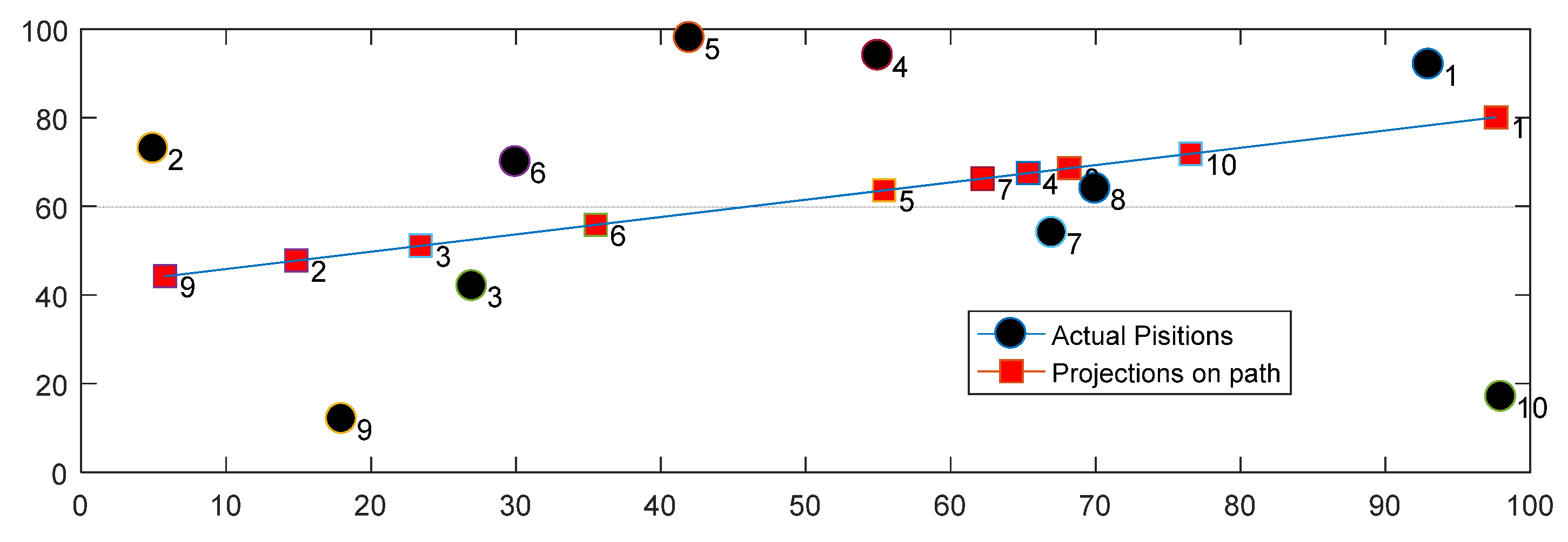
• The projection points are reconstructed using Equation (11) to get their approximate locations on the line.

  $${Reconstruct}_{10\times 2}=\left[\begin{array}{c}97.64 80.11\\ 14.85 47.77\\ 23.43 51.12\\ 65.35 67.50\\ 55.42 63.62\\ 35.52 55.85\\ 62.20 66.27\\ 68.19 68.61\\ 5.79 44.23\\ 76.55 71.88\end{array}\right]$$
• A fixed path for the MS that passes through the reconstructed projection points is generated, as shown in Figure 2.
• The projection points for nodes 9 and 1 are assigned as the start and end points for the MS path, respectively.

3.3. Data Gathering Modes

In our approach, two modes are proposed to gather the data from the sensor nodes after generating the path. These modes are: PCA-direct and PCA-multihop. In the PCA-direct mode, the sensor nodes send their data directly to the MS, while in the PCA-multihop mode, the MS collects the data from certain nodes called rendezvous points. In this section, we discuss the requirements of the two modes in terms of the MS buffer size, the velocity of the MS, and the data rate. Assume the length of the generated path is L, where L is calculated as:

$$\mathrm{L}=\sqrt{{\left(X_{sp}-X_{ep}\right)}^2+{\left(Y_{sp}-Y_{ep}\right)}^2}$$

(12)

where $\left(X_{sp},Y_{sp}\right)$ is the location of the starting point, and $\left(X_{ep},Y_{ep}\right)$ is the location of the end point over the generated path. Moreover, assume $ds$_i is the distance between the projection point for sensor node i and the start point of the MS path. Then,$ds$_i is calculated as:

$$d{s}_{\mathrm{i}}=\sqrt{{\left(X_{sp}-X{p}_i\right)}^2+{\left(Y_{sp}-Y{p}_i\right)}^2}$$

(13)

Additionally, assume $de$_i is the distance between the projection point for sensor node i and the end point of the MS path. Then, $de$_i is given as:

$$d{e}_{\mathrm{i}}=\sqrt{{\left(X_{ep}-X{p}_i\right)}^2+{\left(Y_{ep}-Y{p}_i\right)}^2}$$

(14)

Let V be the MS velocity, and R in bit/second is the rate of taking readings from the environment.

3.3.1. PCA-Direct

In this mode, the MS collects the data directly from each sensor node while it moves back and forth over the generated path. The distance between the projection point for each sensor node and the actual location of that node represents the minimum distance between the sensor node and the MS when it moves over the generated path. Based on that, the MS builds a transmission time schedule (TTS) to inform all sensor nodes about the times in which they should transmit their data.

We assume that the TTS is built such that some sensor nodes are scheduled to transmit their data when the MS moves from the start point to the end point, and the other sensor nodes send their data to the MS while it moves from the end point to the start point. This two-way movement of the MS composes one round. Therefore, the distance that is covered by each round is:

$$D=2\ast L$$

(15)

and the time required for each round is:

$$T=D/V$$

(16)

$$T=2\ast L/V$$

(17)

Therefore, the TTS for each sensor node in the first round can be calculated as follows. For sensor node i, the starting time for sending its data, when the MS moves from the start point to the projection point of sensor node I, is given as follows:

$$T_i^1=dsi/V$$

(18)

$$T_i^1=\frac{\sqrt{{\left(X_{sp}-X{p}_i\right)}^2+{\left(Y_{sp}-Y{p}_i\right)}^2}}{V}$$

(19)

where ($X{p}_i,Y{p}_i$) is the projection point for sensor node i. If sensor node i is scheduled to send its data when the MS moves from the end point to the start point, then the starting time for sensor node i to send its data to the MS in the first round is given as:

$$T_i^1=\frac{\sqrt{{\left(X_{ep}-X{p}_i\right)}^2+{\left(Y_{ep}-Y{p}_i\right)}^2}}{V}+L/V$$

(20)

For the other rounds, the starting time for sensor node i to send its data in round j,$T_i^j$, is given as:

$$T_i^j=T_i^1+\left(j-1\right)\ast T$$

(21)

$$T_i^j=T_i^1+\left(j-1\right)\ast 2L/V$$

(22)

To avoid the buffer overflow that may occur at sensor nodes or the MS, the sensor nodes and the MS will be provided with enough buffer size. The size of the required buffer for each sensor node i is:

$$C_i=R\ast T$$

(23)

while the size of the required buffer for the MS is:

$$C_{MS}=number of sensor noeds\ast C_i$$

(24)

3.3.2. PCA-Multihop

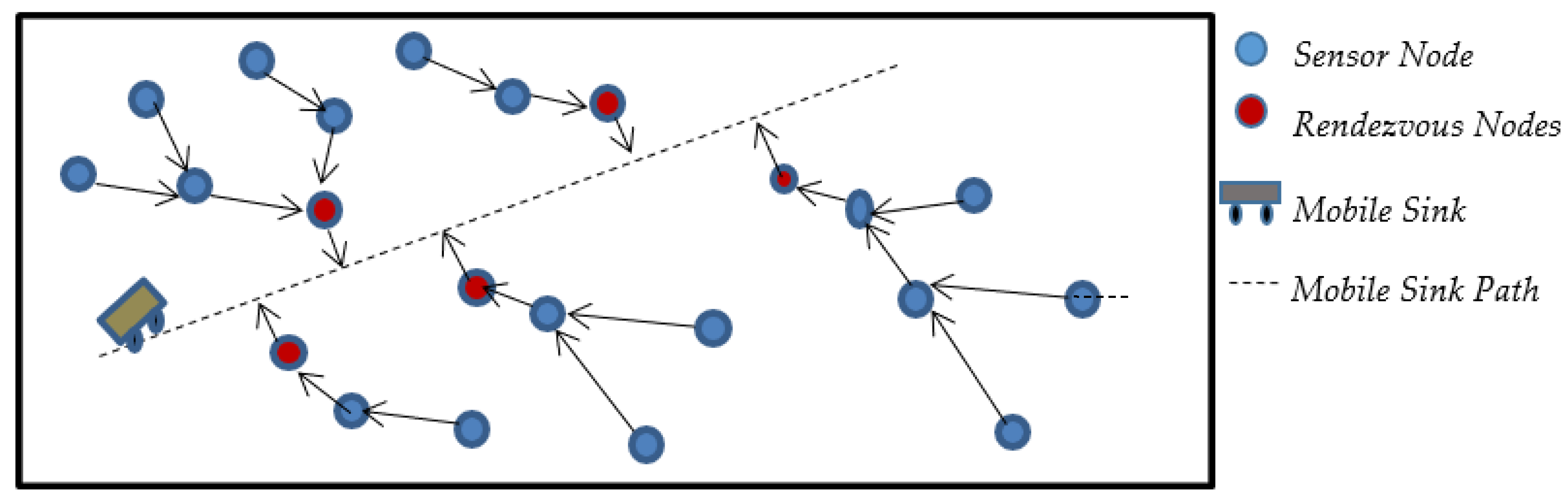
Unfortunately, in the PCA-direct data-gathering mode, the energy of the sensor nodes that are located far from the MS path will be depleted faster than the energy of the sensors nodes that are close to the MS path. Thus, the network’s lifetime would be affected negatively. The multihop mode has been proposed for saving the energy of the far sensor nodes as much as possible, in which it can adjust their transmission range. In PCA-multihop mode, the data of the far sensor nodes will be aggregated at rendezvous points (RPs) via intermediate sensor nodes.

The rendezvous points are subsets of sensor nodes that are located near the MS path and are selected by the MS to be the agents for data delivery. While the MS moves over its generated path, it only contacts these rendezvous points. Other normal sensor nodes can deliver their data to the rendezvous points using the multihop technique, and then the rendezvous points forward those data to the MS directly. Thus, many trees will be constructed in the network, such that the root of each tree will be a rendezvous point and the leaves of these trees will be the farthest nodes from the path, as shown in Figure 3.

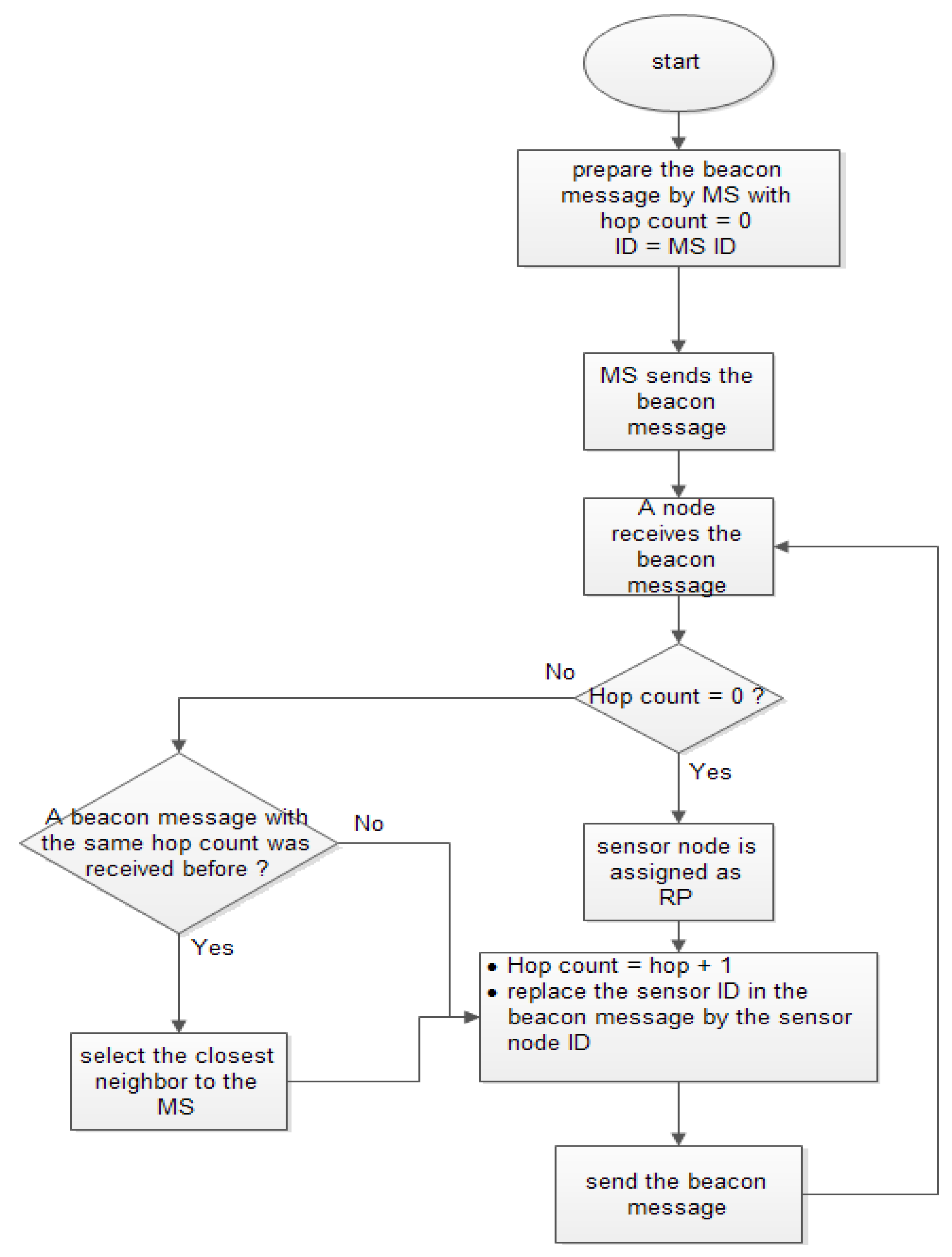
To construct the delivery tree in the multihop mod, the MS moves along the generated path and broadcasts a beacon message within a limited range. The beacon message consists of three parameters: the ID of the node that sends the beacon message, the hop counter, and the distance between the node that sends the beacon message and its projection point.

Each sensor node that receives the beacon message will replace the sender ID with its own ID and increment the hop count by 1 as well as its distance from its projection points before forwarding it to its neighbors and so on. If the sensor node receives the beacon message directly from the MS, it will reply to the MS to declare itself as an RP. Each sensor node that cannot receive the beacon message directly from the MS will select one that has the lowest hop count from its neighbors. If there is more than one neighbor with the same number of hop count, it will select the closest neighbor to the MS path to be its destination. The flowchart shown in Figure 4 summarizes the tree construction.

To avoid the buffer overflow that may occur at rendezvous points or any nodes, the sensor nodes will be provided with enough buffer size. Assume a set of sensor nodes form a tree that is rooted at an RP sensor node. Assume the level is the tree depth. The buffer capacity for the node RP that is required to collect the data from the sensor nodes in the tree as well as its own data is:

$$C_{RP}={\displaystyle \sum }_{k=0}^{level}number of nodes\ast \left(T\ast R\right)$$

(25)

$$C_{RP}={\displaystyle \sum }_{k=0}^{level}number of nodes\ast \left(\frac{2L}{V}\ast R\right)$$

(26)

where level = hop count + 1.

Since the sensor nodes are homogenous, the sensor nodes in the same tree will be provided with a buffer queue (see the results in Equation (26)). Furthermore, the maximum buffer size that is required for one of RPs will be taken as a suitable buffer size for all sensor nodes. After the tree construction, the MS will generate the TTS for the rendezvous points, as explained in Section 4.2.2. To ensure that the data have been collected at each RP before the MS arrives, each RP will generate its own TTS to its children sensor nodes; additionally, each child node will generate a TTS and send that to its children sensor nodes and so on.

4. Performance Evaluation

4.1. Simulation Experiments

We evaluate the performance of the proposed approach under different network configurations. The performance of the proposed data collection modes, PCA-direct and PCA-multihop, are compared against the MECA protocol [15] as this reference is the most similar one that employs direct and multihop modes. The MATLAB tool was used in order to simulate the proposed approach and produce the results. The first-order model, which is discussed in [8], was used to estimate the energy required for receiving or transmitting a k-bit message by the sensor nodes.

Table 3. List of common parameters used in the simulation.

Parameter	Value
Data Packet Size	800 bits
Initial Energy	0.1 J
Eelec	50 nJ/bit
Eamp	10 pJ/bit/m2
Deployment Method	Uniform

shows the common parameters that were used in the simulation.

The following metrics were used to evaluate the performance and compare the proposed protocol with the MECA protocol.

• Number of live nodes: This metric represents the number of live sensor nodes per round.
• Remaining energy: This metric represents the remaining energy as the average remaining energy for live nodes per round.
• Standard deviation of remaining energy: This metric was used to determine how the consumed energy is distributed among the live sensor nodes.
• First dead node: This metric represents the number of elapsed rounds until one of the sensor nodes depletes its whole energy.

In this section, we explain the experiments that have been conducted in order to demonstrate the performance of the proposed approach. Three simulation experiments with different network configurations were used, such that each experiment aims at studying the effect of certain parameters on the proposed approach’s performance. The objectives of these experiments are:

• Demonstrate how the PCA achieves the best path:

The main objective of using the PCA is to generate a path that decreases the distance between the sensor nodes and the MS. In this experiment, we show how the PCA will generate a path for the MS that has a minimal square distance and that can deal with any shape of the network. We evaluate the performance of using the path that was generated by the PCA-based algorithm against the diagonal and horizontal paths.

2.

Study the effect of transmission range:

The transmission range is considered one of the key factors that can affect network performance when the PCA-multihop mode is used. In this experiment, we evaluate the effect of the transmission range on network performance as well as compare the PCA-multihop with PCA-direct and MECA algorithms in terms of the number of live nodes, average remaining energy, and distribution of energy consumption.

3.

Study the effect of network size on the performance of PCA and MECA:

When the network size increases, the distance between the MS and the far nodes will increase too. In this case, the PCA-direct mode will not be an efficient method to send the data to the MS. Therefore, PCA-multihop could perform better than PCA-direct. This experiment aims at studying the effect of the network size on the performance of the proposed approach, especially the PCA-multihop mode.

4.2. Results and Discussion

The results of the four experiments are presented and discussed in this section. Each experiment was repeated 50 times, and the average values of the metrics are considered.

4.2.1. Experiment 1: Demonstrate How PCA Achieves the Best Path

In this experiment, we demonstrate the performance of the proposed PCA-based path generation approach compared with the cases where diagonal and horizontal paths were used. In this experiment, two network sizes, (100 × 100) and (200 × 100), were used.

Table 4. Start and end points for diagonal and horizontal paths.

Network Size	Diagonal Path		Horizontal Path
	Start Point	End Point	Start Point	End Point
100 × 100	(0,0)	−100,100	(0,50)	(100,50)
200 × 100	(0,0)	−200,100	(0,50)	(200,50)

shows the start and end points of the diagonal and horizontal paths. In this experiment, 100 nodes are randomly deployed in the sensing field.

Table 5. Average square distance of PCA-based, diagonal, and horizontal paths.

Network Size	PCA-Based Path	Diagonal Path	Horizontal Path
	(PCA-Direct Mode)
100 × 100	750	892	896
200 × 100	820	1294	803

shows a comparison between the PCA-based generated path (direct mode) and the diagonal and horizontal paths in terms of average square distance. As shown, the PCA-direct mode has a minimum average of square distance in the two cases. That explains the results presented in Figure 5 and Figure 6, which evaluate the PCA-direct mode compared with the diagonal and horizontal paths in terms of the number of live nodes. Figure 5 presents the results when the network size is (100 × 100). The figure shows that the horizontal path outperforms the PCA-direct and diagonal paths in terms of the first dead node. The first dead node starts in the diagonal path first, then the PCA-direct path, and then the horizontal path. This result is because the maximum distance between the farthest node and the MS path in the horizontal path is less than in the diagonal and PCA-direct paths. In the horizontal path, the maximum distance between the farthest node and its projection does not exceed 50, while in the diagonal and PCA-direct paths, the maximum distance could be the distance from one corner to the other center and thus will exceed 50. As shown, the PCA-direct path has a number of live nodes larger than the diagonal and horizontal paths in most of the rounds due to the average square distance that is shown in Table 5.

Figure 6 presents the results when the network size is (200 × 100). As shown, the performance of the PCA-direct path is close to horizontal path and outperforms the diagonal path due to the average square distance that is shown in Table 5.

4.2.2. Experiment 2: Study the Effect of Transmission Range

This experiment aims at evaluating the performance of the proposed approach using the multihop mode. The transmission ranges used in this experiment are 20 and 30 m. In this experiment, we compare the proposed approach using PCA-direct mode, PCA-multihop mode, and the MECA approach.

Table 6. List of parameters used in Experiment 2.

Network Area	100 m * 100 m
Number of sensor nodes	100 nodes
Transmission range for PCA-multihop	20 m, 30 m

shows the parameters that were used in this experiment.

Figure 7 and Figure 8 present the results in terms of live nodes for the transmission ranges of 20 and 30 m, respectively. Figure 7 shows that the proposed PCA-direct mode outperforms the multihop mode and the MECA approach in most simulation rounds. This result is due to two reasons: the network size is small, and the MS moves inside the network. In other words, the MS is close to the sensor nodes. According to the energy defined in the first-order model [8], if the distance between the sender and the receiver is relatively small, the direct transmission is the optimal transmission approach due to the multihop approach consuming extra energy when forwarding the data.

In Figure 8, the first dead node appears earlier in the multihop mode, then in the MECA, and later in the PCA-direct mode. However, the PCA-multihop mode outperforms the PCA-direct mode and the MECA approach in the rest of the simulation rounds because, in multihop mode, the far nodes save some energy that will extend their lifetime.

Furthermore, at the beginning of the simulation, we noticed that the MECA approach outperforms the PCA-multihop mode by about 1500 extra rounds due to the MECA approach using the clustering concept. However, after 1500 rounds, the PCA-multihop approach outperforms the MECA approach and keeps dominating it until the simulation ends.

Figure 8 shows the performance of the three approaches at the transmission range of 30 m. As can be noticed, the PCA-multihop mode is improved. This improvement can be justified due to the increase in transmission distance and, hence, the decrease in the number of relay nodes.

Figure 9 and Figure 10 present the results in terms of the average remaining energy of live nodes for the transmission ranges of 20 and 30 m, respectively. As can be seen at the beginning, the average remaining energy in the PCA-multihop mode is less than in the PCA-direct mode. The reason for this observation is that at the beginning of the simulation, there are no dead nodes, and thus the relay nodes consumed extra energy. After the relay nodes begin dying, the energy consumed by these nodes will decrease, which will cause the average remaining energy in the PCA-multihop mode to become more than in the PCA-direct mode. In addition, the PCA-multihop and PCA-direct modes have better average remaining energy than the MECA approach in all simulation rounds due to the MECA approach using the clustering concept that consumes more energy than PCA-direct and PCA-multihop modes when the MS is close to the sensor nodes.

Figure 11 and Figure 12 present the results in terms of the distribution of energy consumption for transmission ranges of 20 and 30 m, respectively. We measure the distribution of energy by the mean of standard deviation of remaining energy for live nodes per round. As shown in Figure 11, the standard derivation for the PCA-multihop mode increases more than in the PCA-direct mode and the MECA approach. This increase comes from the relay nodes that consume a larger amount of energy in the PCA-multihop mode compared to the far nodes in the PCA-direct mode. We can also see that the distribution of the energy for the MECA approach is close to the PCA-direct mode because of the nature of MECA operation—it merges the clustering concept with direct and multihop communication. Note that the oscillation in the PCA-multihop curve is due to the dying of relay nodes.

Figure 12 shows an improvement in energy distribution for the PCA-multihop mode; the number of relay nodes decreases because the communication range becomes larger, and so the energy consumption becomes more uniform among the nodes, causing the distribution of energy to become both smoother and lower.

4.2.3. Experiment 3: Study the Effect of Network Size

This experiment evaluates the performance of the PCA-multihop mode using two network sizes: (200 m × 200 m) and (500 m × 500 m). In this experiment, the number of sensor nodes is 100, and the transmission range for PCA-multihop is 70 m. Figure 13 and Figure 14 present the results in terms of the number of live nodes per round for network sizes 200 m × 200 m and 500 m × 500 m, respectively. Although the first dead node occurred firstly in PCA-multihop, the comparison between Figure 13 and Figure 14 with Figure 7 shows clearly the amount of improvement in PCA-multihop over PCA-direct and MECA in most of the simulation rounds. We can conclude that PCA-direct and MECA performance decrease gradually as network size increases in size in contrast to small network sizes due to the fact that when the network size increases, the transmission distance increases; according to the energy defined in the first-order model [8], the direct transmission approach will be costly.

Figure 15 and Figure 16 show that the average remaining energy for PCA is much more than MECA due to the use of the clustering method; furthermore, PCA-multihop is better than PCA-direct. From the figures, we can see the PCA-direct remaining energy slope becomes the steepest. This is because of the inverse square relation between communication distance and consumption energy. We also noticed that after the steep curve at the beginning, the PCA-direct curve becomes less steep; this is because the far nodes start dying.

From the results of Experiment 1, and compared with the diagonal and horizontal paths, it has been shown that the best path that the MS sink will use is the one that is constructed based on PCA as this path gives the shortest distance between the sensor nodes and the MS. From the results of Experiment 2, it has been shown that the PCA-direct and PCA-multihop modes have the best performance compared with the MECA approach when the transmission range is considered. However, as the transmission range increases, the PCA-multihop mode dominates the PCA-direct mode because increasing the transmission range will result in a decrease in the number of relay nodes and, therefore, reduce the consumed energy. From the results of Experiment 3, the PCA-direct mode and the MECA approach perform better than the PCA-multihop mode when the network size is small. However, in large-sized networks, the PCA-multihop mode outperforms both the PCA-direct mode and the MECA approach.

5. Conclusions and Future Work

In this paper, we have proposed an efficient path generation algorithm using principal component analysis for mobile sinks in wireless sensor networks. Our main contribution is to generate a path for the MS that has a minimum sum of square distance between the sensor nodes and their projection on the generated path. Two data aggregation modes have been exploited: direct and rendezvous points. We have shown through simulation results that the proposed approach outperforms the diagonal and horizontal paths in terms of the sum of square distance and number of live nodes. Furthermore, the performance of the proposed protocol was compared with another approach called MECA in terms of the number of live nodes, average remaining energy, distribution of energy consumption, and the first dead node. Simulation results showed that the PCA-direct mode performs better than the PCA-multihop mode and MECA in small-sized networks in terms of the number of live nodes and the first dead node, while the PCA-direct mode performs closer to the MECA approach and outperforms the PCA-multihop mode in terms of energy distribution. In networks of large size, the PCA-multihop mode outperforms the PCA-direct mode and the MECA approach in terms of the number of live nodes and average remaining energy, while the MECA approach outperforms the PCA-multihop and PCA-direct modes in terms of the distribution of energy consumption. The experiments also showed that the performance of the PCA-multihop mode is improved when increasing the transmission range due to the decrease in the number of relay nodes that consumed extra energy. Furthermore, a small percentage of improvement is shown in terms of the number of live nodes and distribution of energy consumption in the PCA-multihop mode when increasing node density.

In the future, we aim to make the generated MS path dynamic with respect to remaining energy. We also aim to use multiple mobile sinks to collect the data in order to decrease the communication distance, thus decreasing the consumed energy. Furthermore, we aim to conduct more statistical test analyses on the results, such as the methods presented in [25], and study the effect of different simulation parameters on the results when these parameters are considered together.

References

1. Abdur, R.M.; Arafatur, R.M.; Rahman, M.M.; Asyhari, A.; Bhuiyane, M.; Ramasamy, D. Evolution of IoT-enabled connectivity and applications in automotive industry: A review. Veh. Commun. 2021, 27, 100285. [Google Scholar] [CrossRef]
2. Catarinucci, L.; De Donno, D.; Mainetti, L.; Palano, L.; Patrono, L.; Stefanizzi, M.L.; Tarricone, L. An IoT-aware architecture for smart healthcare systems. IEEE Internet Things J. 2015, 2, 515–526. [Google Scholar] [CrossRef]
3. Ramadan, R.A. Efficient intrusion detection algorithms for smart cities-based wireless sensing technologies. J. Sens. Actuator Netw. 2020, 9, 39. [Google Scholar] [CrossRef]
4. Kaur, L.; Kaur, R. A survey on energy efficient routing techniques in WSNs focusing IoT applications and enhancing fog computing paradigm. Glob. Transit. Proc. 2021, 2, 520–529. [Google Scholar] [CrossRef]
5. Halgamuge, M.N.; Zukerman, M.; Ramamohanarao, K. An estimation of sensor energy consumption. Prog. Electromagn. Res. B 2009, 12, 259–295. [Google Scholar] [CrossRef] [Green Version]
6. Alnawafa, E.; Marghescu, I. New energy efficient multi-hop routing techniques for wireless sensor networks: Static and dynamic techniques. Sensors 2018, 18, 1863. [Google Scholar] [CrossRef] [PubMed] [Green Version]
7. Navarro, M.; Davis, T.W.; Villalba, G.; Li, Y.; Zhong, X.; Erratt, N.; Liang, X.; Liang, Y. Towards long-term multi-hop WSN deployments for environmental monitoring: An experimental network evaluation. J. Sens. Actuator Netw. 2014, 3, 297–330. [Google Scholar] [CrossRef] [Green Version]
8. Heinzelman, W.R.; Chandrakasan, A.; Balakrishnan, H. Energy-efficient communication protocol for wireless micro sensor networks. In Proceedings of the 33rd Annual Hawaii International Conference on System Sciences, Maui, HI, USA, 4–7 January 2000; pp. 1–10. [Google Scholar] [CrossRef]
9. Dong, Q.; Dargie, W. A survey on mobility and mobility-aware MAC protocols in wireless sensor networks. IEEE Commun. Surv. Tutor. 2012, 15, 88–100. [Google Scholar] [CrossRef]
10. Khan, A.W.; Abdullah, A.H.; Anisi, M.H.; Bangash, J.I. A Comprehensive Study of Data Collection Schemes Using Mobile Sinks in Wireless Sensor Networks. Sensors 2014, 14, 2510–2548. [Google Scholar] [CrossRef]
11. Jolliffe, I.T. Principal Component Analysis, 2nd ed.; Springe: New York, NY, USA, 2002; pp. 30–33. [Google Scholar] [CrossRef]
12. Nakayama, H.; Fadlullah, Z.M.; Ansari, N.; Kato, N. A novel scheme for WSAN sink mobility based on clustering and set packing techniques. IEEE Trans. Autom. Control 2011, 56, 2381–2389. [Google Scholar] [CrossRef]
13. Kaswan, A.; Nitesh, K.; Jana, P.K. Energy efficient path selection for mobile sink and data gathering in wireless sensor networks. AEU Int. J. Electron. Commun. 2017, 73, 110–118. [Google Scholar] [CrossRef]
14. Tashtarian, F.; Hossein, M.; Moghaddam, Y.; Effat, S. Energy efficient data gathering algorithm in hierarchical wireless sensor networks with mobile sink. In Proceedings of the 2nd International eConference on Computer and Knowledge Engineering (ICCKE), Mashhad, Iran, 18–19 October 2012; pp. 232–237. [Google Scholar]
15. Wang, J.; Yin, Y.; Kim, J.; Lee, S.; Lai, C. A mobile-sink based energy-efficient clustering algorithm for wireless sensor networks. In Proceedings of the IEEE 12th International Conference on Computer and Information Technology, Chengdu, China, 17–29 October 2012; pp. 678–683. [Google Scholar] [CrossRef]
16. Rakhshan, N.; Rafsanjani, M.K. Improving network lifetime using a MS with a new energy efficiency and minimum delay movement strategy for WSNs. J. Basic Appl. Sci. Res. 2012, 2, 4275–4281. [Google Scholar]
17. Konstantopoulos, C.; Pantziou, G.; Gavalas, D.; Mpitziopoulos, A.; Mamalis, B. A rendezvous-based approach enabling energy-efficient sensory data collection with Mobile Sinks. IEEE Trans. Parallel Distrib. Sys. 2012, 23, 809–817. [Google Scholar] [CrossRef]
18. Xing, G.; Li, M.; Wang, T.; Jia, W.; Huang, J. Efficient rendezvous algorithms for mobility-enabled wireless sensor networks. IEEE Trans. Mob. Comput. 2012, 1, 47–60. [Google Scholar] [CrossRef]
19. Park, J.; Moon, K.; Yoo, S.; Lee, S. Optimal stop points for data gathering in sensor networks with mobile sinks. Wirel. Sens. Netw. 2012, 4, 8–17. [Google Scholar] [CrossRef] [Green Version]
20. Seino, W.; Yoshihisa, T.; Hara, T.; Nishio, S. A sensor data collection method with a mobile sink for communication traffic reduction by delivering predicted values. In Proceedings of the 26th International Conference on Advanced Information Networking and Applications Workshops, Fukuoka, Japan, 26–29 March 2012; pp. 613–618. [Google Scholar]
21. Alnabelsi, S.; Almasaeid, H.; Kamal, A. Optimized sink mobility for energy and delay efficient data collection in FWSNs. In Proceedings of the IEEE Symposium on Computers and Communications (ISCC), Riccione, Italy, 22–25 June 2010; pp. 550–555. [Google Scholar]
22. Safia, A.A.; Aghbari, Z.A.; Kamel, I. Efficient data collection by mobile sink to detect phenomena in internet of things. Information 2017, 8, 123. [Google Scholar] [CrossRef] [Green Version]
23. Najjar-Ghabel, S.; Farzinvash, L.; Razavi, S. Mobile sink-based data gathering in wireless sensor networks with obstacles using artificial intelligence algorithms. Ad. Hoc. Netw. 2020, 106, 102243. [Google Scholar] [CrossRef]
24. Taqieddin, E.; Banimelhem, O.; Shatnawi, I. A path generation algorithm for mobile sinks in wireless sensor networks. In Proceedings of the 9th International Conference on Innovations in Information Technology (IIT), Al Ain, United Arab Emirates, 17–19 March 2013; pp. 164–168. [Google Scholar] [CrossRef]
25. Wei, L.M.; Yu, -T.W.; Jing, G.; Wei, -C.H. Chaos cloud quantum bat hybrid optimization algorithm. Nonlinear Dyn. 2021, 103, 1167–1193. [Google Scholar] [CrossRef]
Figure 1. Ten sensor nodes deployed randomly in a WSN with size (100 × 100).
Jsan 10 00069 g001
Figure 2. The PCA-based generated path for the 10 randomly placed nodes.
Jsan 10 00069 g002
Figure 3. PCA-multihop data collection mode.
Jsan 10 00069 g003
Figure 4. Flowchart for tree construction in PCA-multihop mode.
Jsan 10 00069 g004
Figure 5. Number of live nodes for PCA-direct, diagonal, and horizontal paths (network size 100 × 100).
Jsan 10 00069 g005
Figure 6. Number of live nodes for PCA-direct, diagonal, and horizontal paths (network size 200 × 100).
Jsan 10 00069 g006
Figure 7. Number of live nodes for PCA-multihop, PCA-direct, and MECA (transmission range 20 m).
Jsan 10 00069 g007
Figure 8. Number of live nodes for PCA-multihop, PCA-direct, and MECA (transmission range 30 m).
Jsan 10 00069 g008
Figure 9. Average remaining energy for live nodes for PCA-multihop, PCA-direct, and MECA (transmission range 20 m).
Jsan 10 00069 g009
Figure 10. Average remaining energy for live nodes for PCA-multihop, PCA-direct- and MECA (transmission range 30 m).
Jsan 10 00069 g010
Figure 11. Standard deviation per live node (transmission range 20 m).
Jsan 10 00069 g011
Figure 12. Standard deviation per live node (transmission range 30 m).
Jsan 10 00069 g012
Figure 13. Number of live nodes for PC-multihop, PCA-direct, and MECA (network size 200 m × 200 m).
Jsan 10 00069 g013
Figure 14. Number of live nodes for PC-multihop, PCA-direct, and MECA (network size 500 m × 500 m).
Jsan 10 00069 g014
Figure 15. Average remaining energy for live nodes for PCA-multihop, PCA-direct, and MECA (network size 200 m × 200 m).
Jsan 10 00069 g015
Figure 16. Average remaining energy for live nodes for PCA-multihop, PCA-direct, and MECA (network size 500 m × 500 m).
Jsan 10 00069 g016