Distribution Pattern of Gymnosperms’ Richness in Nepal: Effect of Environmental Constrains along Elevational Gradients


 ,
,  , , , and
Abstract
1. Introduction
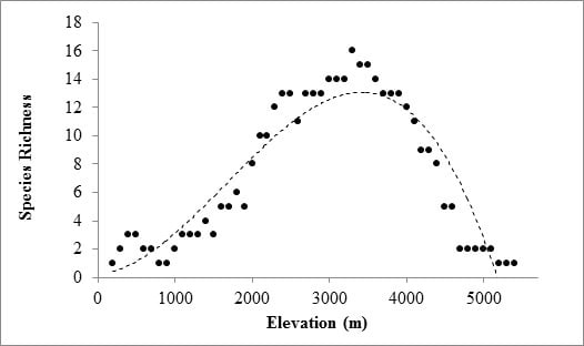
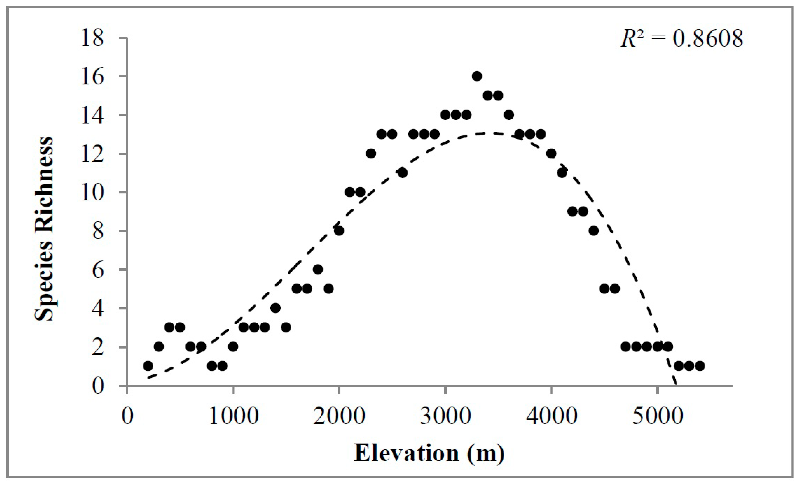
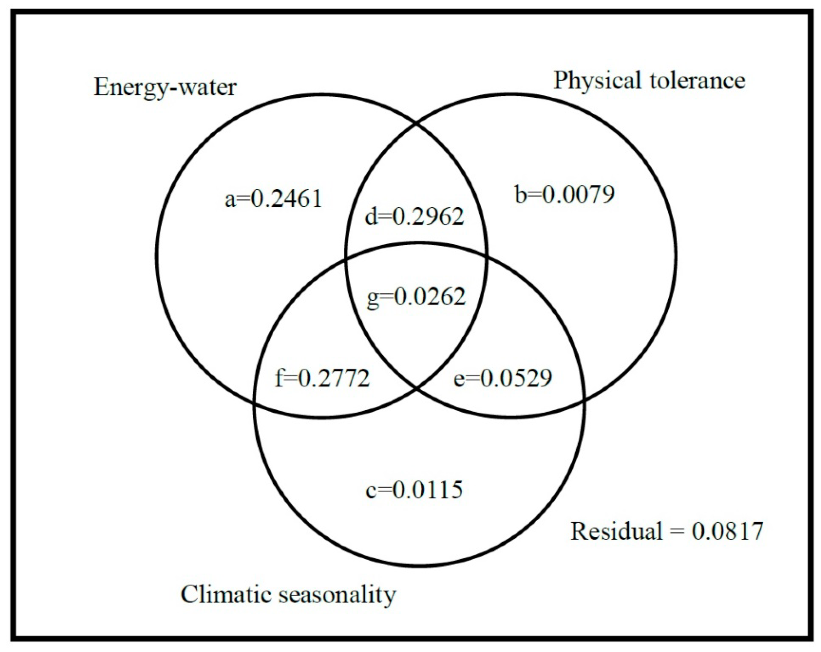
2. Results
3. Discussion
4. Materials and Methods
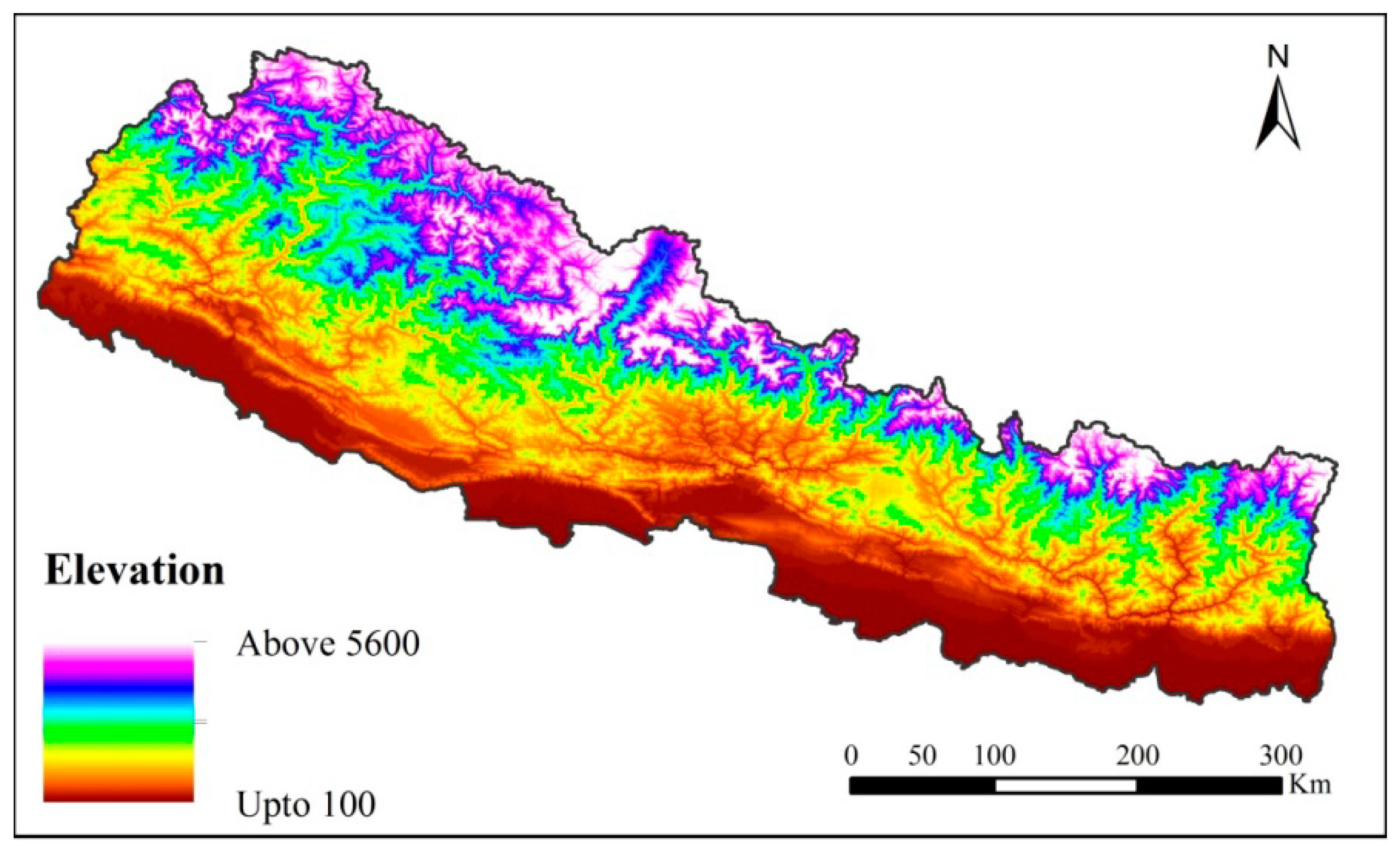
4.1. Study Area and Species Data
4.2. Species Richness
4.3. Predictor Variables
4.4. Statistical Analyses
5. Conclusions
Supplementary Materials
Author Contributions
Funding
Acknowledgments
Conflicts of Interest
References
- Bhattarai, K.R.; Vetaas, O.R. Can Rapoport’s rule explain tree species richness along the Himalayan elevation gradient, Nepal? Divers. Distrib. 2006, 12, 373–378. [Google Scholar] [CrossRef]
- Beck, J.; McCain, C.M.; Axmacher, J.C.; Ashton, L.A.; Bärtschi, F.; Brehm, G.; Choi, S.W.; Cizek, O.; Colwell, R.K.; Fiedler, K. Elevational species richness gradients in a hyperdiverse insect taxon: A global meta-study on geometrid moths. Glob. Ecol. Biogeogr. 2017, 26, 412–424. [Google Scholar] [CrossRef]
- Körner, C. Alpine Plant Life: Functional Plant Ecology of High Mountain Ecosystems; Springer Science & Business Media: Berlin/Heidelberg, Germany, 2003. [Google Scholar]
- Lomolino, M.V. Elevation gradients of species-density: Historical and prospective views. Glob. Ecol. Biogeogr. 2001, 10, 3–13. [Google Scholar] [CrossRef]
- Acebey, A.R.; Krömer, T.; Kessler, M. Species richness and vertical distribution of ferns and lycophytes along an elevational gradient in Los Tuxtlas, Veracruz, Mexico. Flora 2017, 235, 83–91. [Google Scholar] [CrossRef]
- Rahbek, C. The elevational gradient of species richness: A uniform pattern? Ecography 1995, 18, 200–205. [Google Scholar] [CrossRef]
- Vetaas, O.R.; Paudel, K.P.; Christensen, M. Principal factors controlling biodiversity along an elevation gradient: Water, energy and their interaction. J. Biogeogr. 2019, 46, 1652–1663. [Google Scholar] [CrossRef]
- Sanders, N.J. Elevational gradients in ant species richness: Area, geometry, and Rapoport’s rule. Ecography 2002, 25, 25–32. [Google Scholar] [CrossRef]
- Wu, Y.; Yang, Q.; Wen, Z.; Xia, L.; Zhang, Q.; Zhou, H. What drives the species richness patterns of non-volant small mammals along a subtropical elevational gradient? Ecography 2013, 36, 185–196. [Google Scholar] [CrossRef]
- Kessler, M.; Herzog, S.K.; Fjeldså, J.; Bach, K. Species richness and endemism of plant and bird communities along two gradients of elevation, humidity and land use in the Bolivian Andes. Divers. Distrib. 2001, 7, 61–77. [Google Scholar] [CrossRef]
- Krömer, T.; Acebey, A.; Kluge, J.; Kessler, M. Effects of altitude and climate in determining elevational plant species richness patterns: A case study from Los Tuxtlas, Mexico. Flora 2013, 208, 197–210. [Google Scholar] [CrossRef]
- Laiolo, P.; Pato, J.; Obeso, J.R. Ecological and evolutionary drivers of the elevational gradient of diversity. Ecol. Lett. 2018, 21, 1022–1032. [Google Scholar] [CrossRef] [PubMed]
- Paudel, P.K.; Sipos, J.; Brodie, J.F. Threatened species richness along a Himalayan elevational gradient: Quantifying the influences of human population density, range size, and geometric constraints. BMC Ecol. 2018, 18, 6. [Google Scholar] [CrossRef] [PubMed]
- Vetaas, O.R.; Grytnes, J.A. Distribution of vascular plant species richness and endemic richness along the Himalayan elevation gradient in Nepal. Glob. Ecol. Biogeogr. 2002, 11, 291–301. [Google Scholar] [CrossRef]
- De Andrade Kamimura, V.; de Moraes, P.L.R.; Ribeiro, H.L.; Joly, C.A.; Assis, M.A. Tree diversity and elevational gradient: The case of Lauraceae in the Atlantic Rainforest. Flora 2017, 234, 84–91. [Google Scholar] [CrossRef]
- Nascimbene, J.; Marini, L. Epiphytic lichen diversity along elevational gradients: Biological traits reveal a complex response to water and energy. J. Biogeogr. 2015, 42, 1222–1232. [Google Scholar] [CrossRef]
- Acharya, K.P.; Vetaas, O.R.; Birks, H. Orchid species richness along Himalayan elevational gradients. J. Biogeogr. 2011, 38, 1821–1833. [Google Scholar] [CrossRef]
- Baniya, C.B.; Solhøy, T.; Gauslaa, Y.; Palmer, M.W. The elevation gradient of lichen species richness in Nepal. Lichenologist 2010, 42, 83–96. [Google Scholar] [CrossRef]
- Bertuzzo, E.; Carrara, F.; Mari, L.; Altermatt, F.; Rodriguez-Iturbe, I.; Rinaldo, A. Geomorphic controls on elevational gradients of species richness. Proc. Natl. Acad. Sci. USA 2016, 113, 1737–1742. [Google Scholar] [CrossRef]
- Bhattarai, K.R.; Vetaas, O.R.; Grytnes, J.A. Fern species richness along a central Himalayan elevational gradient, Nepal. J. Biogeogr. 2004, 31, 389–400. [Google Scholar] [CrossRef]
- Gao, J.; Zhang, X.; Luo, Z.; Lan, J.; Liu, Y. Elevational diversity gradients across seed plant taxonomic levels in the Lancang River Nature Reserve: Role of temperature, water and the mid-domain effect. J. For. Res. 2017, 29, 1121–1127. [Google Scholar] [CrossRef]
- Gong, H.; Yu, T.; Zhang, X.; Zhang, P.; Han, J.; Gao, J. Effects of boundary constraints and climatic factors on plant diversity along an altitudinal gradient. Glob. Ecol. Conserv. 2019, 19, e00671. [Google Scholar] [CrossRef]
- Hoiss, B.; Krauss, J.; Steffan-Dewenter, I. Interactive effects of elevation, species richness and extreme climatic events on plant–pollinator networks. Glob. Chang. Biol. 2015, 21, 4086–4097. [Google Scholar] [CrossRef] [PubMed]
- Kluge, J.; Worm, S.; Lange, S.; Long, D.; Böhner, J.; Yangzom, R.; Miehe, G. Elevational seed plants richness patterns in Bhutan, Eastern Himalaya. J. Biogeogr. 2017, 44, 1711–1722. [Google Scholar] [CrossRef]
- Li, M.; Feng, J. Biogeographical interpretation of elevational patterns of genus diversity of seed plants in Nepal. PLoS ONE 2015, 10, e0140992. [Google Scholar] [CrossRef] [PubMed]
- Grau, O.; Grytnes, J.A.; Birks, H. A comparison of altitudinal species richness patterns of bryophytes with other plant groups in Nepal, Central Himalaya. J. Biogeogr. 2007, 34, 1907–1915. [Google Scholar] [CrossRef]
- Wu, Z.; Raven, P. Flora of China, Vol. 4 (Cycadaceae through Fagaceae); Science Press and Missouri Botanical Garden Press: Beijing, China; St. Louis, MO, USA, 1999. [Google Scholar]
- Hawkins, B.A.; Field, R.; Cornell, H.V.; Currie, D.J.; Guégan, J.-F.; Kaufman, D.M.; Kerr, J.T.; Mittelbach, G.G.; Oberdorff, T.; O’Brien, E.M. Energy, water, and broad-scale geographic patterns of species richness. Ecology 2003, 84, 3105–3117. [Google Scholar] [CrossRef]
- O’Brien, E.M. Biological relativity to water–energy dynamics. J. Biogeogr. 2006, 33, 1868–1888. [Google Scholar] [CrossRef]
- Gao, J.; Liu, Y. Climate stability is more important than water–energy variables in shaping the elevational variation in species richness. Ecol. Evol. 2018, 8, 6872–6879. [Google Scholar] [CrossRef]
- Currie, D.J.; Mittelbach, G.G.; Cornell, H.V.; Field, R.; Guégan, J.F.; Hawkins, B.A.; Kaufman, D.M.; Kerr, J.T.; Oberdorff, T.; O’Brien, E. Predictions and tests of climate-based hypotheses of broad-scale variation in taxonomic richness. Ecol. Lett. 2004, 7, 1121–1134. [Google Scholar] [CrossRef]
- Kreyling, J.; Schmid, S.; Aas, G. Cold tolerance of tree species is related to the climate of their native ranges. J. Biogeogr. 2015, 42, 156–166. [Google Scholar] [CrossRef]
- Spasojevic, M.J.; Grace, J.B.; Harrison, S.; Damschen, E.I. Functional diversity supports the physiological tolerance hypothesis for plant species richness along climatic gradients. J. Ecol. 2014, 102, 447–455. [Google Scholar] [CrossRef]
- Chan, W.-P.; Chen, I.-C.; Colwell, R.K.; Liu, W.-C.; Huang, C.-Y.; Shen, S.-F. Seasonal and daily climate variation have opposite effects on species elevational range size. Science 2016, 351, 1437–1439. [Google Scholar] [CrossRef] [PubMed]
- Shrestha, N.; Su, X.; Xu, X.; Wang, Z. The drivers of high Rhododendron diversity in south-west China: Does seasonality matter? J. Biogeogr. 2017, 45, 438–447. [Google Scholar] [CrossRef]
- Bhattarai, K.R.; Vetaas, O.R. Variation in plant species richness of different life forms along a subtropical elevation gradient in the Himalayas, east Nepal. Glob. Ecol. Biogeogr. 2003, 12, 327–340. [Google Scholar] [CrossRef]
- Dhital, M.R. Geology of the Nepal Himalaya: Regional Perspective of the Classic Collided Orogen; Springer: Berlin/Heidelberg, Germany, 2015. [Google Scholar]
- Paudel, P.K.; Bhattarai, B.P.; Kindlmann, P. An overview of the biodiversity in Nepal. In Himalayan Biodiversity in the Changing World; Kindlmann, P., Ed.; Springer: Berlin/Heidelberg, Germany, 2012. [Google Scholar]
- Gaire, N.; Koirala, M.; Bhuju, D.; Borgaonkar, H. Treeline dynamics with climate change at the central Nepal Himalaya. Clim. Past. 2014, 10, 1277–1290. [Google Scholar] [CrossRef]
- Choi, S.W. Patterns of an elevational gradient affecting moths across the South Korean mountains: Effects of geometric constraints, plants, and climate. Ecol. Res. 2016, 31, 321–331. [Google Scholar] [CrossRef]
- Mu, Q.; Heinsch, F.A.; Zhao, M.; Running, S.W. Development of a global evapotranspiration algorithm based on MODIS and global meteorology data. Remote Sens. Environ. 2007, 111, 519–536. [Google Scholar] [CrossRef]
- Vetaas, O.R.; Ferrer-Castán, D. Patterns of woody plant species richness in the Iberian Peninsula: Environmental range and spatial scale. J. Biogeogr. 2008, 35, 1863–1878. [Google Scholar] [CrossRef]
- Panda, R.M.; Behera, M.D.; Roy, P.S.; Biradar, C. Energy determines broad pattern of plant distribution in Western Himalaya. Ecol. Evol. 2017, 7, 10850–10860. [Google Scholar] [CrossRef]
- Trisurat, Y.; Shrestha, R.P.; Kjelgren, R. Plant species vulnerability to climate change in Peninsular Thailand. Appl. Geogr. 2011, 31, 1106–1114. [Google Scholar] [CrossRef]
- Ohlemüller, R.; Anderson, B.J.; Araújo, M.B.; Butchart, S.H.; Kudrna, O.; Ridgely, R.S.; Thomas, C.D. The coincidence of climatic and species rarity: High risk to small-range species from climate change. Biol. Lett. 2008, 4, 568–572. [Google Scholar] [CrossRef] [PubMed]
- Telwala, Y.; Brook, B.W.; Manish, K.; Pandit, M.K. Climate-induced elevational range shifts and increase in plant species richness in a Himalayan biodiversity epicentre. PLoS ONE 2013, 8, e57103. [Google Scholar] [CrossRef] [PubMed]
- Dakhil, M.A.; Xiong, Q.; Farahat, E.A.; Zhang, L.; Pan, K.; Pandey, B.; Olatunji, O.A.; Tariq, A.; Wu, X.; Zhang, A. Past and future climatic indicators for distribution patterns and conservation planning of temperate coniferous forests in southwestern China. Ecol. Indic. 2019, 107, 105559. [Google Scholar] [CrossRef]
- Xu, W.; Svenning, J.C.; Chen, G.; Chen, B.; Huang, J.; Ma, K. Plant geographical range size and climate stability in China: Growth form matters. Glob. Ecol. Biogeogr. 2018, 27, 506–517. [Google Scholar] [CrossRef]
- Dobremez, J.-F. Le Népal, Écologie et Biogéographie; Centre National de la Rechereche Scientifique: Paris, France, 1976. [Google Scholar]
- Shrestha, K.; Bhattarai, S.; Bhandari, P. Handbook of Flowering Plants of Nepal (Vol. 1 Gymnosperms and Angiosperms: Cycadaceae-Betulaceae); Scientific Publishers: Jodhpur, India, 2018. [Google Scholar]
- Press, J.R.; Shrestha, K.K.; Sutton, D.A. Annotated Checklist of the Flowering Plants of Nepal; Natural History Museum Publications: London, UK, 2000. [Google Scholar]
- McCain, C.M. The mid-domain effect applied to elevational gradients: Species richness of small mammals in Costa Rica. J. Biogeogr. 2004, 31, 19–31. [Google Scholar] [CrossRef]
- Rosenzweig, M.L. Species Diversity in Space and Time; Cambridge University Press: Cambridge, UK, 1995. [Google Scholar]
- Hu, Y.; Ding, Z.; Jiang, Z.; Quan, Q.; Guo, K.; Tian, L.; Hu, H.; Gibson, L. Birds in the Himalayas: What drives beta diversity patterns along an elevational gradient? Ecol. Evol. 2018, 8, 11704–11716. [Google Scholar] [CrossRef]
- Farr, T.G.; Rosen, P.A.; Caro, E.; Crippen, R.; Duren, R.; Hensley, S.; Kobrick, M.; Paller, M.; Rodriguez, E.; Roth, L. The shuttle radar topography mission. Rev. Geophys. 2007, 45. [Google Scholar] [CrossRef]
- Jiang, Z.; Ma, K.; Anand, M. Can the physiological tolerance hypothesis explain herb richness patterns along an elevational gradient? A trait-based analysis. Community Ecol. 2016, 17, 17–23. [Google Scholar] [CrossRef]
- Hijmans, R.J.; Cameron, S.E.; Parra, J.L.; Jones, P.G.; Jarvis, A. Very high resolution interpolated climate surfaces for global land areas. Int. J. Climatol. 2005, 25, 1965–1978. [Google Scholar] [CrossRef]
- Moura, M.R.; Villalobos, F.; Costa, G.C.; Garcia, P.C.A. Disentangling the Role of Climate, Topography and Vegetation in Species Richness Gradients. PLoS ONE 2016, 11, e0152468. [Google Scholar] [CrossRef]
- Anderson, D.R.; Burnham, K.P. Avoiding pitfalls when using information-theoretic methods. J. Wildl. Manag. 2002, 66, 912–918. [Google Scholar] [CrossRef]
- Legendre, P.; Legendre, L. Numerical Ecology; Elsevier: Amsterdam, The Netherlands, 2012. [Google Scholar]
- D’Agostino, R. Goodness-of-Fit-Techniques; CRC Press: Boca Raton, FL, USA, 1986. [Google Scholar]
- Murray, K.; Conner, M.M. Methods to quantify variable importance: Implications for the analysis of noisy ecological data. Ecology 2009, 90, 348–355. [Google Scholar] [CrossRef] [PubMed]
- Legendre, P. Studying beta diversity: Ecological variation partitioning by multiple regression and canonical analysis. J. Plant Ecol. 2007, 1, 3–8. [Google Scholar] [CrossRef]
- R Development Core Team. R: A Language and Environment for Statistical Computing; R Foundation for Statistical Computing: Vienna, Austria, 2017. [Google Scholar]


| Hypotheses | Predictor Variables Included in The Best Model (Coefficient of Variables) | Percentage of Coefficient of Determination (% of R2adj) | p-Value | AIC |
|---|---|---|---|---|
| Energy-Water | EW1 (−0.2968) *** | 77.93 | <0.001 | 219.9 |
| EW2 (+0.4821) *** | ||||
| EW3 (−0.6361) *** | ||||
| Physical tolerance | PT1 (−0.2762) ** | 38.64 | <0.001 | 297.2 |
| PT2 (−0.4276) *** | ||||
| Climatic Seasonality | CS2 (−0.6052) *** | 46.80 | <0.001 | 289.1 |
| CS3 (−0.1697) * |
© 2020 by the authors. Licensee MDPI, Basel, Switzerland. This article is an open access article distributed under the terms and conditions of the Creative Commons Attribution (CC BY) license (http://creativecommons.org/licenses/by/4.0/).
Share and Cite
Pandey, B.; Nepal, N.; Tripathi, S.; Pan, K.; Dakhil, M.A.; Timilsina, A.; Justine, M.F.; Koirala, S.; Nepali, K.B. Distribution Pattern of Gymnosperms’ Richness in Nepal: Effect of Environmental Constrains along Elevational Gradients. Plants 2020, 9, 625. https://doi.org/10.3390/plants9050625
Pandey B, Nepal N, Tripathi S, Pan K, Dakhil MA, Timilsina A, Justine MF, Koirala S, Nepali KB. Distribution Pattern of Gymnosperms’ Richness in Nepal: Effect of Environmental Constrains along Elevational Gradients. Plants. 2020; 9(5):625. https://doi.org/10.3390/plants9050625
Chicago/Turabian StylePandey, Bikram, Nirdesh Nepal, Salina Tripathi, Kaiwen Pan, Mohammed A. Dakhil, Arbindra Timilsina, Meta F. Justine, Saroj Koirala, and Kamal B. Nepali. 2020. "Distribution Pattern of Gymnosperms’ Richness in Nepal: Effect of Environmental Constrains along Elevational Gradients" Plants 9, no. 5: 625. https://doi.org/10.3390/plants9050625
APA StylePandey, B., Nepal, N., Tripathi, S., Pan, K., Dakhil, M. A., Timilsina, A., Justine, M. F., Koirala, S., & Nepali, K. B. (2020). Distribution Pattern of Gymnosperms’ Richness in Nepal: Effect of Environmental Constrains along Elevational Gradients. Plants, 9(5), 625. https://doi.org/10.3390/plants9050625