
Morphological Variation and Spatial Distribution Patterns of Krascheninnikovia compacta (Losinsk.) Grubov in the Tibetan Antelope Breeding Grounds of the Western Kunlun Mountains

Abstract

1. Introduction
2. Results
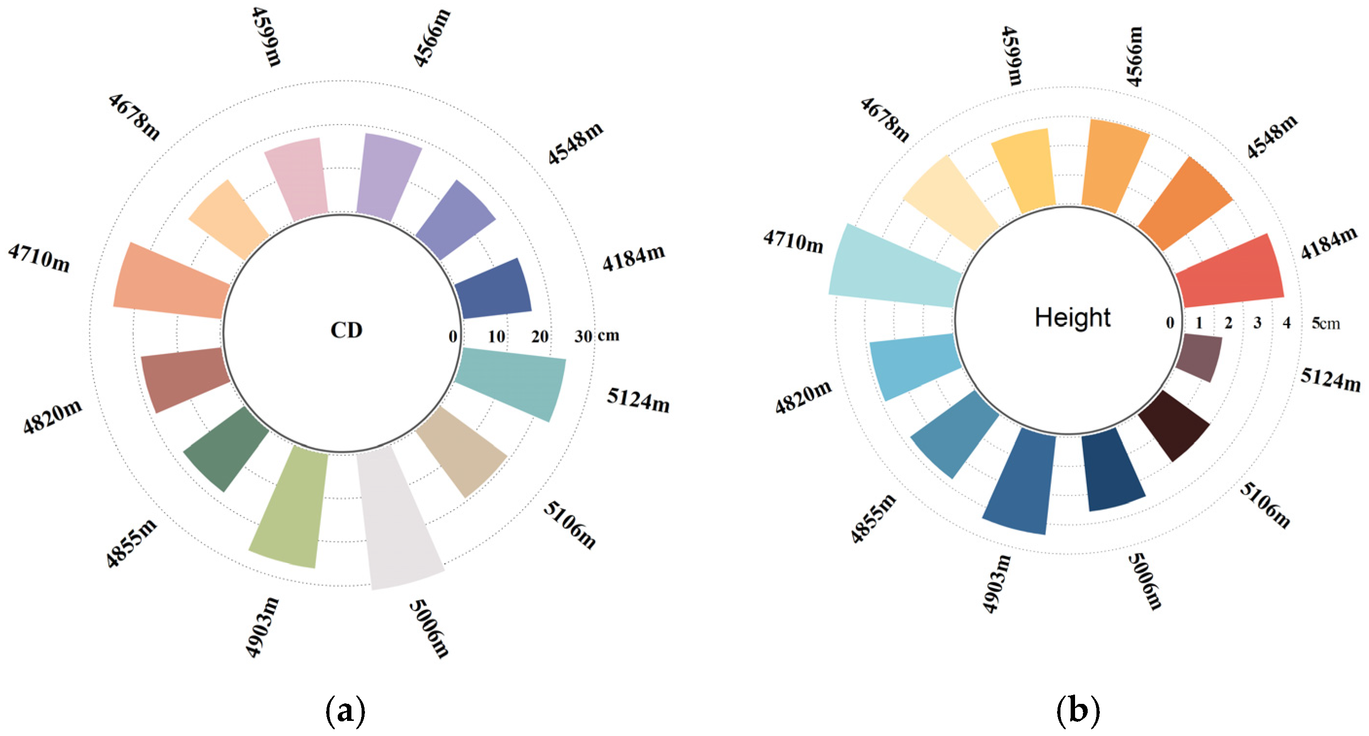
2.1. Statistical Analysis of Plant Height and Crown Diameter
2.2. Morphological Changes of K. compacta
2.2.1. Correlation Between Crown Diameter and Environmental Factors
2.2.2. Correlation Between Plant Height and Environmental Factors
2.2.3. Morphological Responses of Plant Height and Crown Diameter to Environmental Drivers
2.3. Spatial Distribution Pattern of K. compacta
2.3.1. Spatial Density of K. compacta Across Elevational Gradients
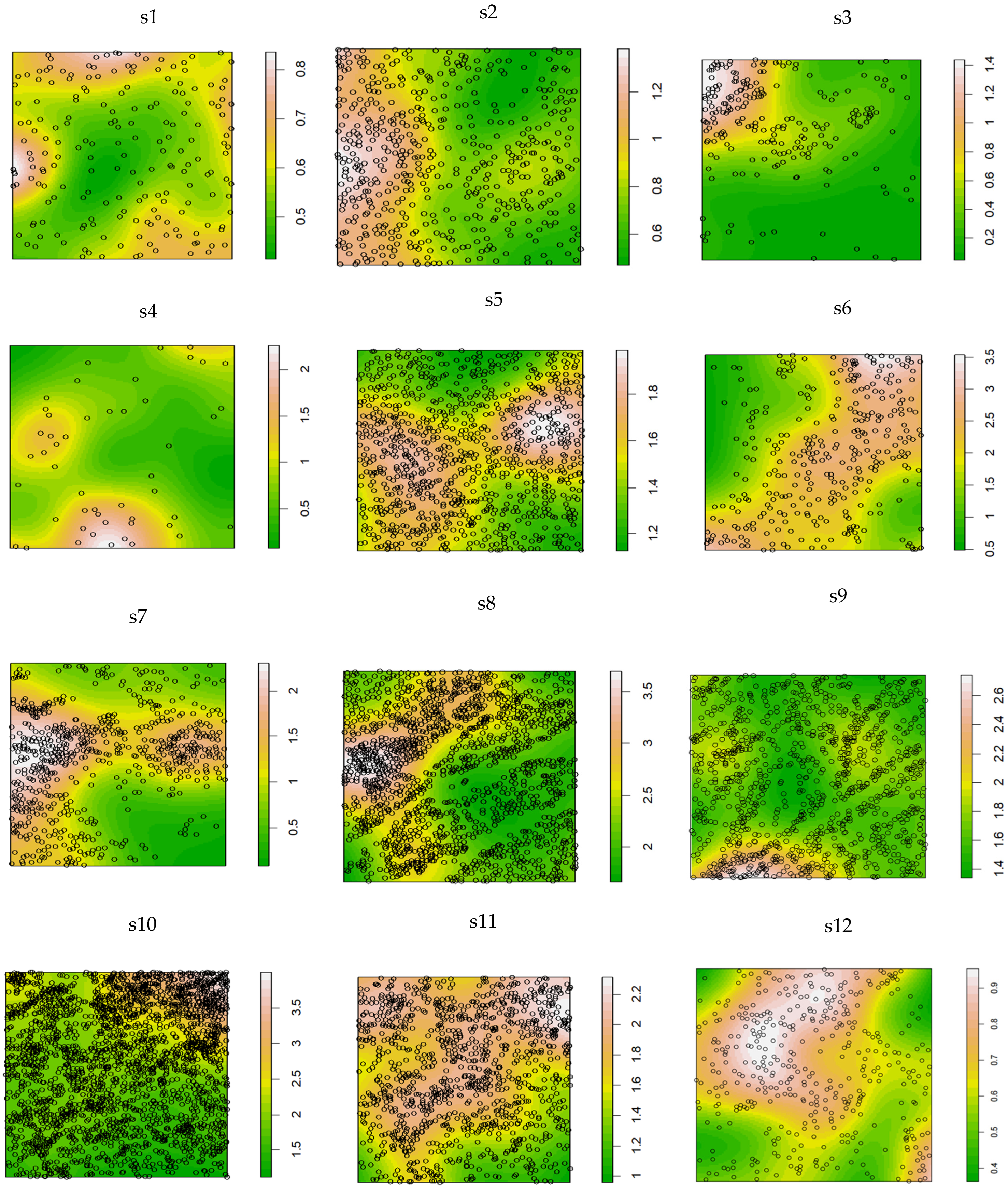
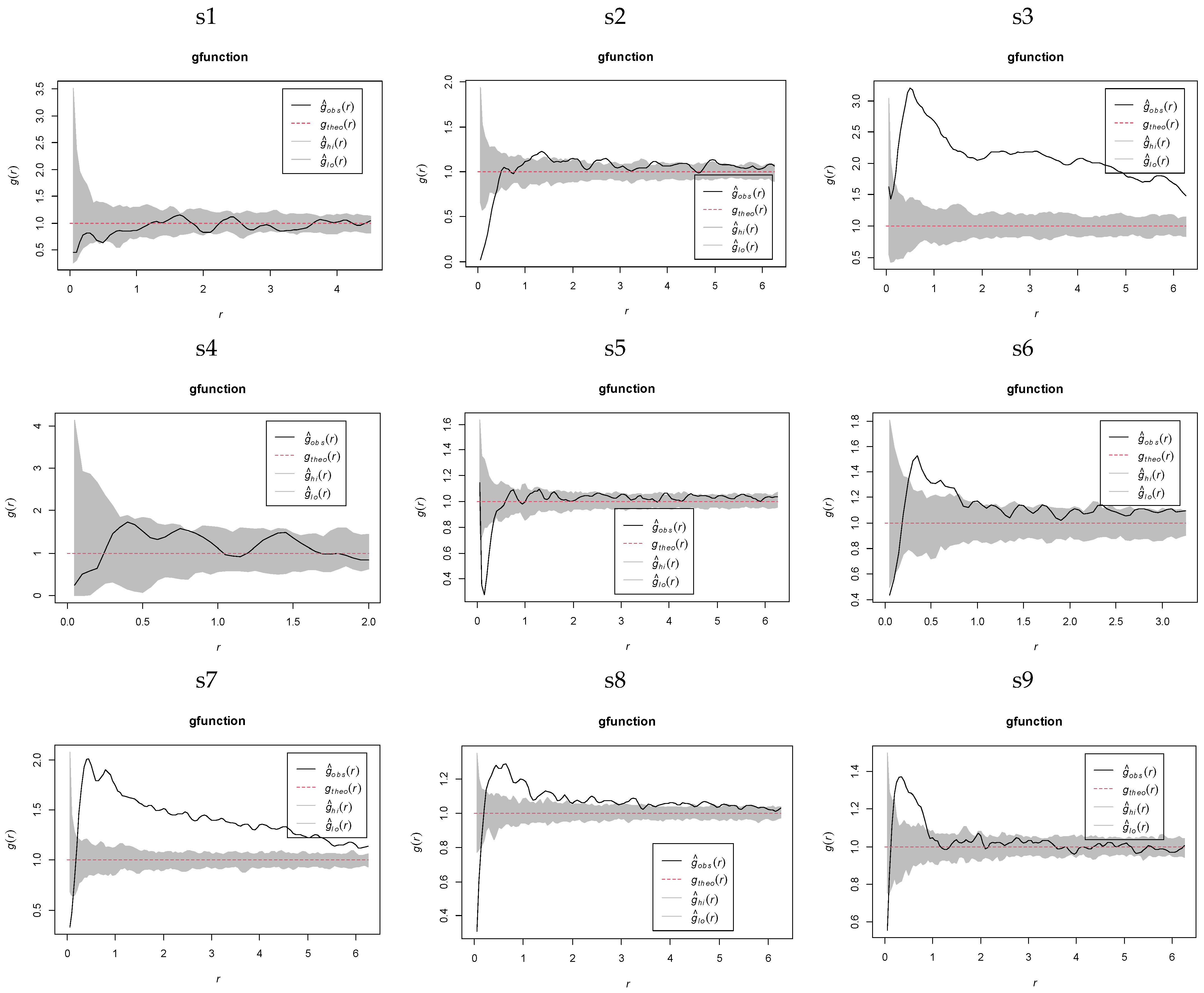
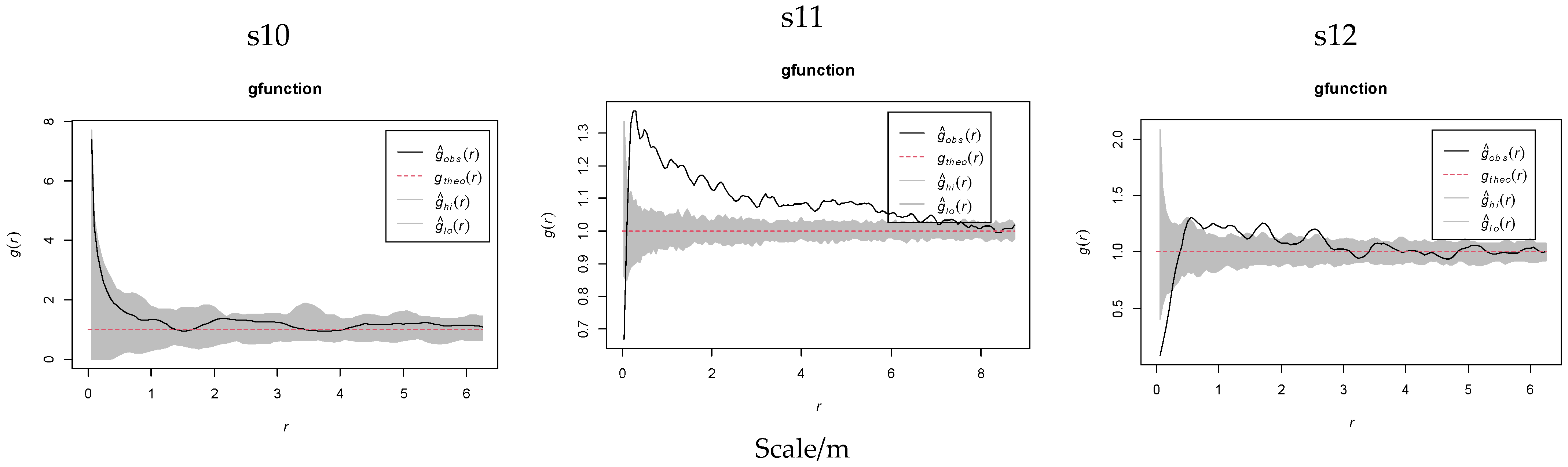
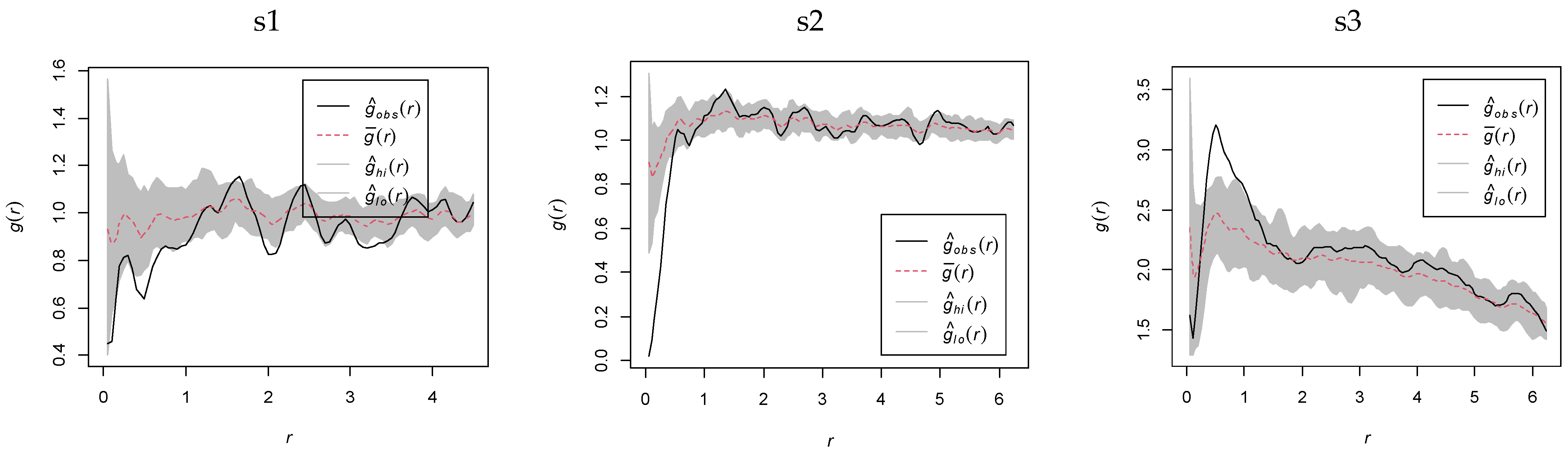
2.3.2. Spatial Distribution Heterogeneity of K. compacta Across Elevational Gradients
2.4. MaxEnt Model Analysis
2.4.1. MaxEnt Model Optimization and Parameter Evaluation
2.4.2. Current and Future Habitat Distribution
3. Discussion
3.1. Adaptive Morphological Plasticity in Plant Height and Crown Diameter of K. compacta
3.2. The Spatial Distribution Pattern of Crown Width and Plant Height in K. compacta
3.3. Prediction of the Suitable Habitat Areas for K. compacta Using MaxEnt
4. Materials and Methods
4.1. Materials
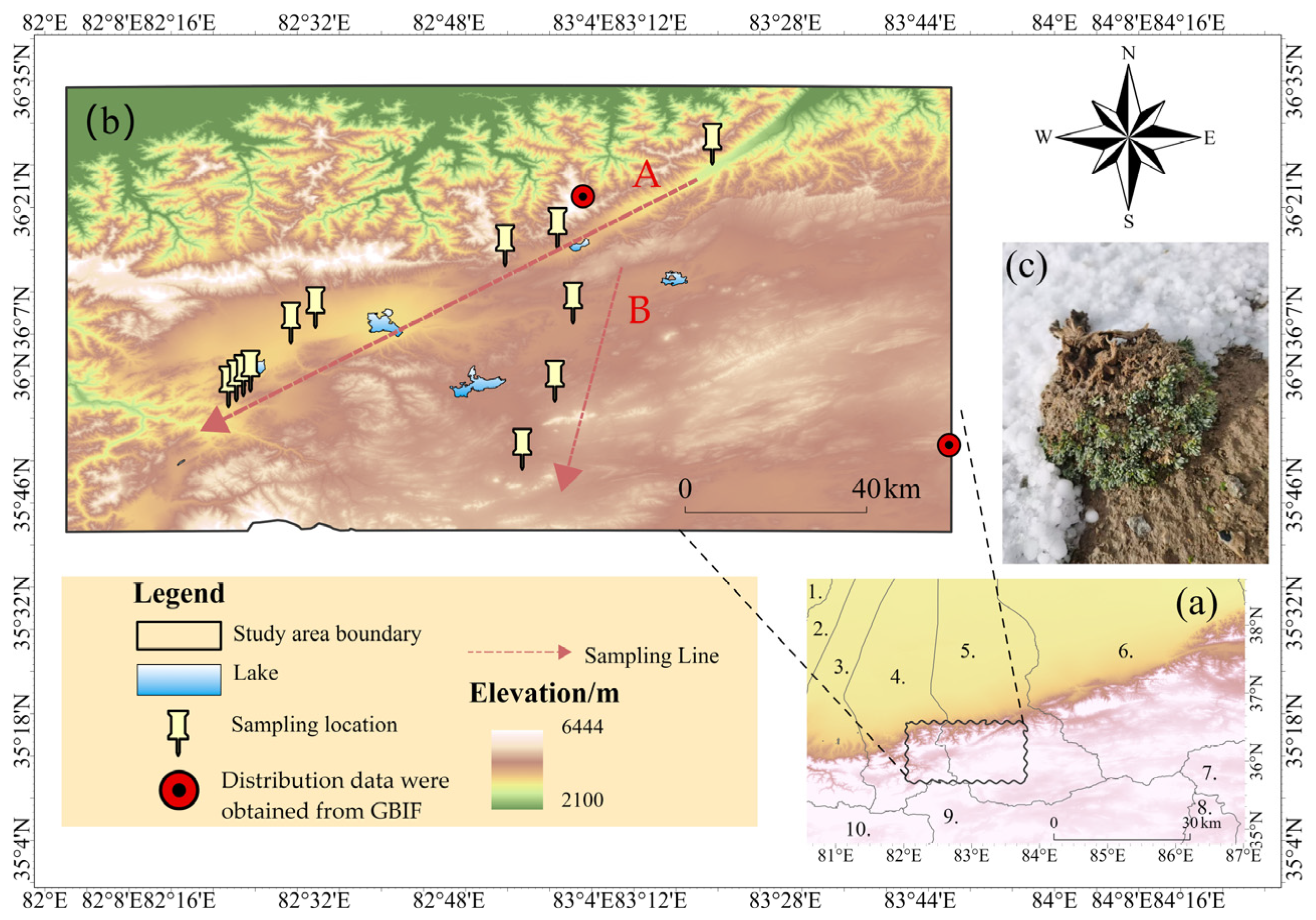
4.1.1. Study Area
4.1.2. Data
4.1.3. Sampling Areas Design
4.1.4. UAV Image Processing
4.1.5. Point Pattern Data Processing
4.1.6. MaxEnt Model Construction and Validation
4.2. Methods
4.2.1. Plasticity Index
4.2.2. Redundancy Analysis
4.2.3. Point Pattern Analysis
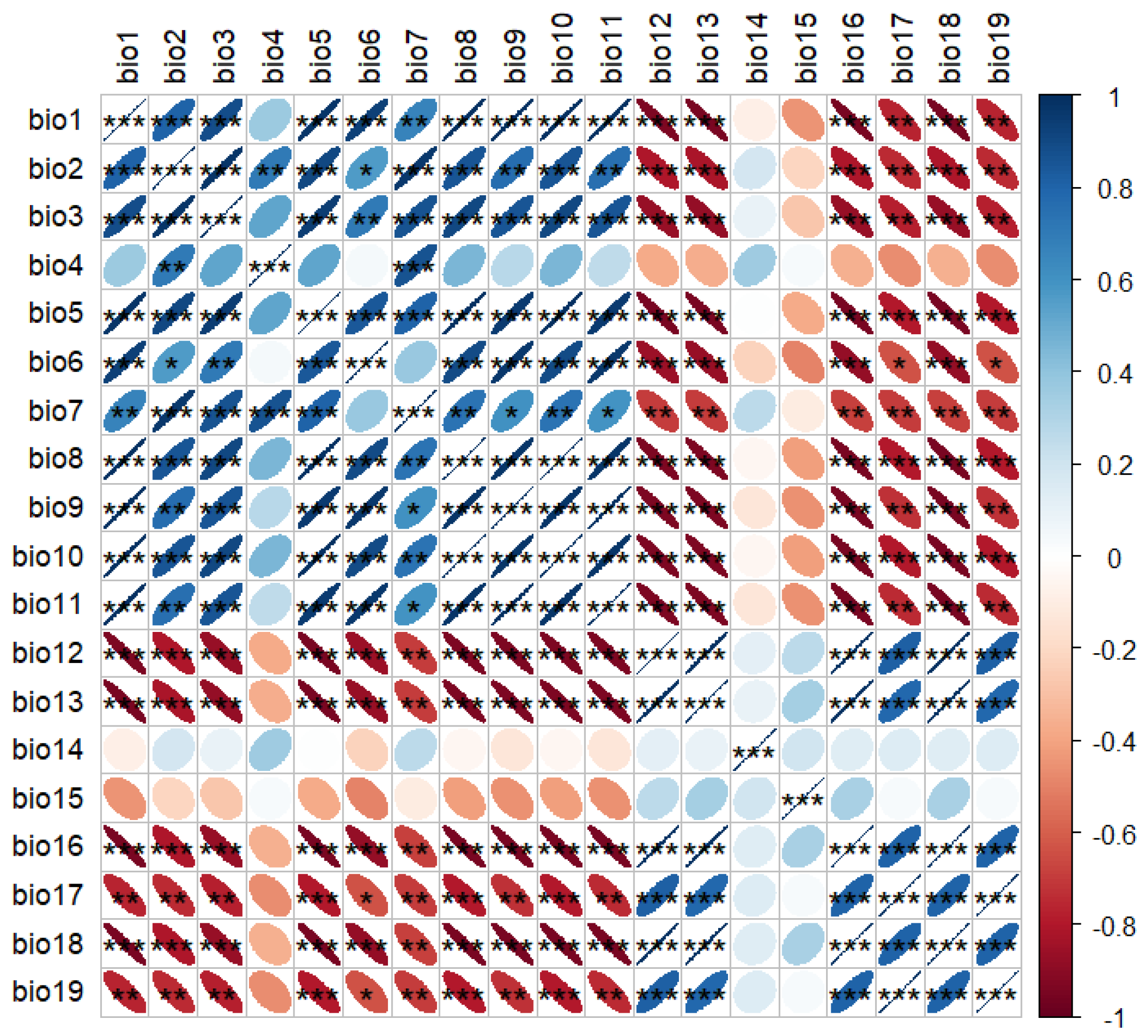
4.2.4. Correlation Analysis
4.2.5. MaxEnt Model
5. Conclusions
Author Contributions
Funding
Data Availability Statement
Acknowledgments
Conflicts of Interest
Abbreviations
| UAV | unmanned aerial vehicle |
| DOM | digital orthophoto map |
| DSM | digital surface model |
| DEM | digital elevation model |
| CSR | complete spatial randomness |
| HP | heterogeneous Poisson |
| PI | plasticity index |
| RDA | redundancy analysis |
| DCA | detrended correspondence analysis |
| MAT | mean annual temperature |
| PET | potential evapotranspiration |
| AI | aridity index |
| RH | relative humidity |
| CV | coefficient of variation |
| VIF | variance inflation factor |
| PCC | Pearson correlation coefficient |
| MaxEnt | maximum entropy |
| ROC | operating characteristic curve |
| TPT | balance training omission, predicted area, and threshold value |
| MTSS | maximum training sensitivity plus specificity |
References
- Liu, H.; Gleason, S.M.; Hao, G.; Hua, L.; He, P.; Goldstein, G.; Ye, Q. Hydraulic traits are coordinated with maximum plant height at the global scale. Sci. Adv. 2019, 5, eaav1332. [Google Scholar] [CrossRef] [PubMed]
- Mashau, A.C.; Hempson, G.P.; Lehmann, C.E.R.; Vorontsova, M.S.; Visser, V.; Archibald, S. Plant height and lifespan predict range size in southern African grasses. J. Biogeogr. 2021, 48, 3047–3059. [Google Scholar] [CrossRef]
- Dong, L.; Hu, X.; Yang, W. Study on Crown Prediction Model of Haloxylon ammodendron in Different Habitats. For. Eng. 2024, 40, 1–10. (In Chinese) [Google Scholar]
- Lü, L. Prediction Model for Single-Tree Crown Width of Major Broadleaf Species in the Natural Secondary Forest of Maoershan Mountain. Master’s Thesis, Northeast Forestry University, Harbin, China, 2019. (In Chinese). [Google Scholar]
- Shenkin, A.; Bentley, L.P.; Oliveras, I.; Salinas, N.; Adu-Bredu, S.; Marinmomet-Junior, B.H.; Marimon, B.S.; Peprah, T.; Choque, E.L.; Rodriguez, L.T.; et al. The influence of ecosystem and phylogeny on tropical tree crown size and shape. Front. For. Glob. Change 2020, 3, 501757. [Google Scholar] [CrossRef]
- Maharjan, S.K.; Sterck, F.J.; Dhakal, B.P.; Makri, M.; Poorter, L. Functional traits shape tree species distribution in the Himalayas. J. Ecol. 2021, 109, 3818–3834. [Google Scholar] [CrossRef]
- Niu, C.; Zhang, D.; Zhang, Z.; Wang, Y. Spatial distribution pattern and spatial correlation of main sand-fixing shrubs in fixed dunes in Yanchi region, Mu Us sandy land. Ecol. Sci. 2024, 43, 1–9. (In Chinese) [Google Scholar]
- Tang, R.; Zhang, D.; Zhao, Y.; Shan, L.; Yang, T.; Li, J.; Huang, W. Spatial point pattern of Artemisia ordosica shrubland on fixed sand dunes in the MU Us Sand, Land, China. Chin. J. Ecol. 2025, 1–11. (In Chinese) [Google Scholar] [CrossRef]
- Fordham, D.A.; Resit Akçakaya, H.; Araújo, M.B.; Elith, J.; Keith, D.A.; Peaeson, R.; Auld, T.D.; Morgan, J.W.; Regan, T.J.; Watts, M.J.; et al. Plant extinction risk under climate change: Are forecast range shifts alone a good indicator of species vulnerability to global warming? Glob. Change Biol. 2012, 18, 1357–1371. [Google Scholar] [CrossRef]
- Kumari, P.; Wani, I.A.; Khan, S.; Verma, S.; Mushtaq, S.; Gulnaz, A.; Paray, B.A. Modeling of Valeriana wallichii Habitat Suitability and Niche Dynamics in the Himalayan Region under Anticipated Climate Change. Biology 2022, 11, 498. [Google Scholar] [CrossRef]
- Zhang, H.; Zhao, H.; Wang, H. Potential geographical distribution of populus euphratica in China under future climate change scenarios based on Maxent model. Acta Ecol. Sin. 2020, 40, 6552–6563. (In Chinese) [Google Scholar]
- Leslie, D.M.; Schaller, G.B. Pantholops hodgsonii (Artiodactyla: Bovidae). Mamm. Species 2008, 817, 1–13. [Google Scholar] [CrossRef]
- Schaller, G.B. Wildlife of the Tibetan Steppe; University of Chicago Press: Chicago, IL, USA, 2000. [Google Scholar]
- Wei, Z.; Xu, Z. Habitat distribution of Tibetan antelope in the Chang Tang plateau and influential factors. Acta Ecol. Sin. 2020, 40, 8763–8772. (In Chinese) [Google Scholar]
- Schaller, G.B.; Kang, A.; Cai, X.; Liu, Y. Migratory and calving behavior of Tibetan antelope population. Acta Theriol. Sin. 2006, 2, 105–113. [Google Scholar]
- Zhao, H.; Guo, K.; Qiao, X.; Liu, C. The ecogeographical characteristics of Ceratoides compacta alpine desert on the Tibetan Plateau. Geogr. Res. 2017, 36, 2441–2450. (In Chinese) [Google Scholar]
- Koyro, H.W.; Breckle, S.W. Ecophysiological Constraints Under Salinity Stress: Halophytes Versus Non-Halophytes; Dagar, J.C., Gupta, S.R., Kumar, A., Eds.; Halophytes vis-à-vis Saline Agriculture; Springer: Singapore, 2024; pp. 179–229. [Google Scholar]
- Editorial Committee of Flora of China, Chinese Academy of Sciences. Flora of China; Science Press: Beijing, China, 1979; Volume 25, p. 7. [Google Scholar]
- Aygün, C.; Olgun, M.; Erkara, İ.P.; Koyuncu, O.; Ardic, M.; Sezer, O. Usability of Krascheninnikovia ceratoides, Atriplex canescens, Quercus infectoria and Quercus robur as Feed. Biol. Divers. Conserv. 2020, 3, 209–216. [Google Scholar]
- Seidl, A.; Pérez-Collazos, E.; Tremetsberger, K.; Carine, M.; Catalán, P.; Bernharat, K.L. Phylogeny and biogeography of the Pleistocene Holarctic steppe and semi-desert goosefoot plant Krascheninnikovia ceratoides. Flora 2020, 262, 151504. [Google Scholar] [CrossRef]
- Seidl, A.; Tremetsberger, K.; Pfanzelt, S.; Blattner, F.R.; Neuffer, B.; Friesen, N.; Hurka, H.; Shmakov, A.; Batlai, O.; Čalasan, A.Ž.; et al. The phylogeographic history of Krascheninnikovia reflects the development of dry steppes and semi-deserts in Eurasia. Sci. Rep. 2021, 11, 6645. [Google Scholar] [CrossRef]
- Lomonosova, M.N.; Pankova, T.V.; Korolyuk, E.A.; Shaulo, D.N.; Osmonali, B.; Nikolin, E.G. Nuclear genome size analysis in Krascheninnikovia ceratoides s.l. (Amaranthaceae). Bot. Pacifica. A J. Plant Sci. Conserv. 2024, 13, 183–187. [Google Scholar]
- Arachchige, C.N.P.G.; Prendergast, L.A.; Staudte, R.G. Robust analogs to the coefficient of variation. J. Appl. Stat. 2022, 49, 268–290. [Google Scholar] [CrossRef]
- Zhang, X.; Zhang, W.; Pan, Y.; Quan, W.; Li, M.; He, H.; Zhou, H. Spatiotemporal Trends and Drivers of Vegetation Growth in the Shaanxi Yellow River Basin, 2001–2020. Chin. J. Appl. Ecol. 2025, 36, 341–352. (In Chinese) [Google Scholar]
- Stotz, G.C.; Salgado-Luarte, C.; Escobedo, V.M.; Valladares, F.; Gianoli, E. Global trends in phenotypic plasticity of plants. Ecol. Lett. 2021, 24, 2267–2281. [Google Scholar] [CrossRef] [PubMed]
- Wright, I.J.; Ackerly, D.D.; Bongers, F.; Harms, K.E.; Ibarra-Manriquez, G.; Martinez-Ramos, M.; Mazer, S.J.; Muller-Landau, H.C.; Paz, H.; Pitman, M.C.A.; et al. Relationships among ecologically important dimensions of plant trait variation in seven Neotropica forests. Ann. Bot. 2007, 99, 1003–1015. [Google Scholar] [CrossRef] [PubMed]
- Zhang, Y.; Qian, L.; Chen, X.; Sun, L.; Sun, H.; Chen, J. Diversity patterns of cushion plants on the Qinghai-Tibet Plateau: A basic study for future conservation efforts on alpine ecosystems. Plant Divers. 2022, 44, 231–242. [Google Scholar] [CrossRef]
- Wang, L.; Song, X.; Gu, J.; Shao, X. Relationship between morphological characteristics of Didymodon constrictus and environmental changes in Xizang and its response strategies. Chin. J. Plant Ecol. 2024, 48, 1351–1360. (In Chinese) [Google Scholar]
- Wang, Y.; Sun, J.; Liu, B.; Wang, J.; Zeng, T. Cushion plants as critical pioneers and engineers in alpine ecosystems across the Tibetan Plateau. Ecol. Evol. 2021, 11, 11554–11558. [Google Scholar] [CrossRef] [PubMed]
- Rasray, B.A.; Ahmad, R.; Lone, S.A.; Islam, T.; Wani, S.A.; Hussain, K.; Dar, F.A.; Rai, I.D.; Padalia, H.; Khuroo, A.A. Cushions serve as conservation refuges for the himalayan alpine plant diversity: Implications for nature-based environmental management. J. Environ. Manag. 2024, 359, 120995. [Google Scholar] [CrossRef] [PubMed]
- Sekar, K.C.; Thapliyal, N.; Pandey, A.; Joshi, B.; Mukherjee, S.; Bhojak, P.; Bisht, M.; Bhatt, D.; Singh, S.; Bahukhandi, A.; et al. Plant species diversity and density patterns along altitude gradient covering high-altitude alpine regions of west Himalaya, India. Geol. Ecol. Landsc. 2024, 8, 559–573. [Google Scholar] [CrossRef]
- Chaves, C.J.N.; Cacossi, T.C.; Matos, T.S.; Bento, J.P.S.P.; Goncalves, L.N.; Silva, S.F.; Silva-Ferreira, M.V.; Barbin, D.F.; Mayer, J.L.S.; Sussulini, A.; et al. Bromeliad populations perform distinct ecological strategies across a tropical elevation gradient. Funct. Ecol. 2024, 38, 910–925. [Google Scholar] [CrossRef]
- Li, J.; Gao, H.; Yin, G.; Liang, Z.; Yang, X. Spatial Distribution and Intraspecific Interactions of the Critically Endangered Aquatic Plant Ottelia acuminata var. jingxiensis. Chin. J. Ecol. 2025, 1–7. Available online: http://kns.cnki.net/kcms/detail/21.1148.Q.20250126.1303.022.html (accessed on 20 February 2025). (In Chinese).
- Zhao, R.; Zhang, H.; An, L. Spatial patterns and interspecific relationships of two dominant cushion plants at three elevations on the Kunlun Mountain, China. Environ. Sci. Pollut. Res. 2020, 27, 17339–17349. [Google Scholar] [CrossRef]
- Chen, J.; Shi, Z.; Liu, S.; Zhang, M.; Cao, X.; Chen, M.; Xu, G.; Xing, H.; Li, F.; Feng, Q. Altitudinal Variation Influences Soil Fungal Community Composition and Diversity in Alpine–Gorge Region on the Eastern Qinghai–Tibetan Plateau. J. Fungi 2022, 8, 807. [Google Scholar] [CrossRef] [PubMed]
- Zhao, C.; Gao, F.; Wang, X.; Sheng, Y.; Shi, F. Small-Scale Point Pattern Analysis of the Stellera chamaejasme Population in Degraded Alpine Grasslands of the Upper Heihe Rive. Chin. J. Plant Ecol. 2010, 34, 1319–1326. (In Chinese) [Google Scholar]
- Wu, X.; Zhao, C.; Ma, X.; Wang, S.; Zhang, P.; Huang, C.; Li, G. Spatial pattern and interspecific association of Beckmannia syzigachne and Kobresia tibetica in an alpine peatland. Chin. J. Ecol. 2024, 43, 1621–1628. (In Chinese) [Google Scholar]
- He, X.; Ümüt, H.; Dong, Z.; Yusup, A.; Kurban, A. Spatial distribution pattern and intraspecific competition of Populus euphratica riparian forests under different water gradients. Acta Ecol. Sin. 2023, 43, 7497–7506. (In Chinese) [Google Scholar]
- Jia, X. Chinese Forage Plant Flora; Agriculture Press: Beijing, China, 1992; Volume 4, p. 301. (In Chinese) [Google Scholar]
- Zhang, X.; Wu, M.; Wu, Q.; Wang, D.; Zhang, S. Reviewing the adaptation strategies of clonal plants to heterogeneous habitats. Acta Ecol. Sin. 2022, 42, 4255–4266. (In Chinese) [Google Scholar]
- Li, B.; Liu, M.; Zhang, Y.; Nan, X.; Xia, S. Analysis of Point Patterns of Different Altitude Gradient of Anaphalis lactea and Saussurea hieracioides in Gannan Alpine Meadow. Acta Bot. Boreali-Occident. Sin. 2019, 39, 1472–1479. (In Chinese) [Google Scholar]
- Hao, H.; Si, L.; Yang, G.; Yue, Y.; Zhou, J.; Lai, L.; Zheng, Y. Distribution patterns of the Cupressus gigantea populationsin the Yarlung Tsangpo River and their responses to environmental changes. J. Beijing Norm. Univ. 2024, 60, 594–600. (In Chinese) [Google Scholar]
- Xu, A.; Xu, D.; Liu, L.; Yu, S.; Huang, J.; Mi, S.; Zhu, N. Point pattern analysis of dominant populations based on null models in desert steppe in Ningxia. Acta Ecol. Sin. 2020, 40, 4180–4187. (In Chinese) [Google Scholar]
- Cavieres, L.A.; Sanhueza, C.E.; Hernández-Fuentes, C. Warming had contrasting effects on the importance of facilitative interactions with a cushion nurse species on native and non-native species in the high-Andes of central Chile. Oikos 2024, 2024, e10296. [Google Scholar] [CrossRef]
- Pugnaire, F.I.; Pistón, N.; Macek, P.; Schöb, C.; Estruch, C.; Armas, C. Warming enhances growth but does not affect plant interactions in an alpine cushion species. Perspect. Plant Ecol. Evol. Syst. 2020, 44, 125530. [Google Scholar] [CrossRef]
- Cannone, N.; Malfasi, F.; Favero-Longo, S.E.; Convey, P.; Guglielmin, M. Acceleration of climate warming and plant dynamics in Antarctica. Curr. Biol. 2022, 32, 1599–1606.e2. [Google Scholar] [CrossRef]
- Seastedt, T.R.; Oldfather, M.F. Climate Change, Ecosystem Processes and Biological Diversity Responses in High Elevation Communities. Climate 2021, 9, 87. [Google Scholar] [CrossRef]
- Cui, J.; Li, Z.; Wang, Y.; Sun, Q.; Sha, N.; Li, Z.; Wu, Y.; Shi, Y.; Han, Y.; Li, M.; et al. A dataset describing the community characteristics and geographic distribution of Krascheninnikovia compacta. Biodivers. Sci. 2023, 31, 144–150. (In Chinese) [Google Scholar] [CrossRef]
- Zhang, Y.; Tang, J.; Ren, G.; Zhao, K.; Wang, X. Global potential distribution prediction of Xanthium italicum based on Maxent model. Sci. Rep. 2021, 11, 16545. (In Chinese) [Google Scholar] [CrossRef] [PubMed]
- Dou, Q.; Chen, C.; Zeng, T.; Long, Z.; Miao, Q.; Sun, F.; Cai, R.; Chen, X.; Suo, N. Evaluation of Habitat Suitability of Important Medicinal Plants Gentianaceae in the Qinghai-Tibet Plateau based on the Optimized Maximum Entropy Model. Acta Agrestia Sin. 2025, 4–20. Available online: http://kns.cnki.net/kcms/detail/23.1480.S.20250305.0943.002.html (accessed on 5 March 2025). (In Chinese).
- Feng, Q.; Zhao, W.; Hu, X.; Liu, Y.; Daryanto, S.; Cherubini, F. Trading-off ecosystem services for better ecological restoration: A case study in the Loess Plateau of China. J. Clean. Prod. 2020, 257, 120469. [Google Scholar] [CrossRef]
- Ben-Said, M.; Ghallab, A.; Lamrhari, H.; Carreira, J.A.; Linares, J.C.; Taïqui, L. Characterizing spatial structure of Abies marocana forest through point pattern analysis. For. Syst. 2020, 29, e014. [Google Scholar] [CrossRef]
- Morais, É.T.; Barberes, G.A.; Souza, I.V.A.F.; Leal, F.G.; Guzzo, J.V.P.; Spigolon, A.L.D. Pearson Correlation Coefficient Applied to Petroleum System Characterization: The Case Study of Potiguar and Reconcavo Basins, Brazil. Geosciences 2023, 13, 282. [Google Scholar] [CrossRef]
- Harte, J.; Newman, E.A. Maximum information entropy: A foundation for ecological theory. Trends Ecol. Evol. 2014, 29, 384–389. [Google Scholar] [CrossRef]
- Phillips, S.J.; Anderson, R.P.; Schapire, R.E. Maximum entropy modeling of species geographic distributions. Ecol. Model. 2006, 190, 231–259. [Google Scholar] [CrossRef]


| Sampling Areas | Mean/cm | Max/cm | Min/cm | Kurtosis | Skewness | Standard Deviation | CV/% | PI |
|---|---|---|---|---|---|---|---|---|
| S1 | 15.79 | 18.81 | 10.98 | −0.95 | 0.002 | 1.79 | 11.35 | 0.42 |
| S2 | 24.95 | 35.17 | 16.67 | −0.85 | 0.40 | 4.94 | 19.80 | 0.53 |
| S3 | 31.39 | 44.1 | 19.22 | 0.45 | −0.01 | 5.20 | 16.56 | 0.56 |
| S4 | 18.29 | 20.06 | 13.31 | 2.91 | −1.75 | 1.77 | 9.68 | 0.34 |
| S5 | 17.30 | 24.76 | 9.45 | −0.45 | 0.04 | 3.27 | 18.93 | 0.62 |
| S6 | 17.57 | 23.47 | 13.46 | −0.97 | 0.52 | 3.17 | 18.05 | 0.43 |
| S7 | 18.55 | 27.11 | 12.58 | −0.34 | 0.44 | 3.53 | 19.01 | 0.54 |
| S8 | 16.05 | 23.78 | 9.86 | −0.13 | 0.55 | 2.90 | 18.06 | 0.59 |
| S9 | 15.98 | 25.96 | 8.13 | −0.45 | 0.33 | 3.65 | 22.85 | 0.69 |
| S10 | 26.36 | 37.85 | 13.39 | −1.33 | 0.19 | 8.26 | 31.35 | 0.65 |
| S11 | 23.71 | 36.54 | 15.67 | −0.06 | 0.68 | 5.28 | 22.27 | 0.57 |
| S12 | 19.29 | 25.40 | 10.78 | −0.36 | −0.14 | 3.51 | 18.22 | 0.58 |
| Sampling Areas | Mean/cm | Max/cm | Min/cm | Kurtosis | Skewness | Standard Deviation | CV/% | PI |
|---|---|---|---|---|---|---|---|---|
| S1 | 3.44 | 4.30 | 2.07 | −0.18 | −0.35 | 0.61 | 17.73 | 0.52 |
| S2 | 3.07 | 4.29 | 2.03 | −0.24 | 0.28 | 0.53 | 17.30 | 0.53 |
| S3 | 2.58 | 3.90 | 1.47 | 0.41 | 0.21 | 0.52 | 20.29 | 0.62 |
| S4 | 2.95 | 3.86 | 1.67 | 0.19 | −0.54 | 0.65 | 22.08 | 0.57 |
| S5 | 2.63 | 3.97 | 1.53 | −0.38 | 0.51 | 0.04 | 20.10 | 0.61 |
| S6 | 2.73 | 3.50 | 2.02 | −1.04 | −0.26 | 0.47 | 17.21 | 0.42 |
| S7 | 2.87 | 3.82 | 1.67 | 0.19 | 0.15 | 0.51 | 17.88 | 0.46 |
| S8 | 3.07 | 4.80 | 1.27 | −0.31 | 0.09 | 0.70 | 22.63 | 0.74 |
| S9 | 3.00 | 4.38 | 153 | 0.18 | 0.02 | 0.54 | 17.97 | 0.65 |
| S10 | 3.39 | 4.90 | 1.11 | 1.87 | −0.82 | 0.95 | 28.09 | 0.77 |
| S11 | 1.30 | 2.38 | 0.5 | −0.44 | 0.53 | 0.49 | 37.30 | 0.79 |
| S12 | 2.02 | 2.97 | 1.33 | 0.31 | 0.51 | 0.37 | 18.32 | 0.55 |
| Sampling Areas | Longitudes of Site Center (E) | Latitudes of Site Center (N) | Elevations/m |
|---|---|---|---|
| S1 | 83°19′19.596″ | 36°25′3.475″ | 4184 |
| S2 | 83°0′56.79″ | 36°15′3.658″ | 4710 |
| S3 | 82°54′42.178″ | 36°13′3.626″ | 5006 |
| S4 | 82°32′10.018″ | 36°5′40.945″ | 4566 |
| S5 | 82°29′14.964″ | 36°3′52.103″ | 4599 |
| S6 | 82°24′25.654″ | 35°58′9.746″ | 4855 |
| S7 | 82°23′35.441″ | 35°57′38.902″ | 4820 |
| S8 | 82°22′45.217″ | 35°57′1.804″ | 4678 |
| S9 | 82°21′49.165″ | 35°56′19.036″ | 4548 |
| S10 | 83°2′46.824″ | 36°6′14.551″ | 4903 |
| S11 | 83°0′37.447″ | 35°56′58.085″ | 5124 |
| S12 | 82°56′44.794″ | 35°48′54.158″ | 5106 |
| Environmental Factors | RDA1 | RDA2 | R2 | Pr(>r) |
|---|---|---|---|---|
| Slope | −0.94124 | 0.33773 | 0.1793 | 0.406 |
| MAT | −0.98336 | 0.18166 | 0.8120 | 0.001 *** |
| Texcls | 0.99999 | 0.00452 | 0.4965 | 0.085 |
| RH | 0.94193 | −0.33581 | 0.5237 | 0.051 |
| SAND | 0.99984 | −0.01762 | 0.2308 | 0.296 |
| Light | 0.98632 | −0.16486 | 0.3276 | 0.186 |
| Period | Suitable Habitat/104 km2 | ||
|---|---|---|---|
| Highly Suitable Habitat | Sub-Suitable Habitat | Unsuitable Habitat | |
| 1970 to 2000s | 0.43 | 0.65 | 0.39 |
| 2061 to 2080s (SSP126) | 0.2 | 0.44 | 0.83 |
| 2061 to 2080s (SSP585) | 0.44 | 0.81 | 0.21 |
| Climatic Period | Area/104 km2 | Proportion of Area/% | ||||
|---|---|---|---|---|---|---|
| Expansion | Unchanged | Contraction | Expansion | Unchanged | Contraction | |
| Current-2061 to 2080s (SSP126) | 0.0016 | 0.63 | 0.44 | 0.1 | 43.21 | 30.26 |
| Current-2061 to 2080s (SSP585) | 0.2 | 1.06 | 0.01 | 13.4 | 72.46 | 1 |
| Bioclimatic Variable | Code | Unit |
|---|---|---|
| bio1 | Annual Mean Temperature | °C |
| bio2 | Mean Diurnal Range (Mean of monthly (max temp—min temp) | °C |
| bio3 | Isothermality (bio2/bio7) (×100) | % |
| bio4 | Temperature Seasonality (standard deviation × 100) | °C |
| bio5 | Max Temperature of Warmest Month | °C |
| bio6 | Min Temperature of Coldest Month | °C |
| bio7 | Temperature Annual Range (bio5-bio6) | °C |
| bio8 | Mean Temperature of Wettest Quarter | °C |
| bio9 | Mean Temperature of Driest Quarter | °C |
| bio10 | Mean Temperature of Warmest Quarter | °C |
| bio11 | Mean Temperature of Coldest Quarter | °C |
| bio12 | Annual Precipitation | mm |
| bio13 | Precipitation of Wettest Month | mm |
| bio14 | Precipitation of Driest Month | mm |
| bio15 | Precipitation Seasonality (Coefficient of Variation) | % |
| bio16 | Precipitation of Wettest Quarter | mm |
| bio17 | Precipitation of Driest Quarter | mm |
| bio18 | Precipitation of Warmest Quarter | mm |
| Bio19 | Precipitation of Coldest Quarter | mm |
Disclaimer/Publisher’s Note: The statements, opinions and data contained in all publications are solely those of the individual author(s) and contributor(s) and not of MDPI and/or the editor(s). MDPI and/or the editor(s) disclaim responsibility for any injury to people or property resulting from any ideas, methods, instructions or products referred to in the content. |
© 2025 by the authors. Licensee MDPI, Basel, Switzerland. This article is an open access article distributed under the terms and conditions of the Creative Commons Attribution (CC BY) license (https://creativecommons.org/licenses/by/4.0/).
Share and Cite
Huang, K.; Lai, F.; Chen, M.; Song, Y.; Chen, S.; Wubuaysan, Z.; Zhuang, X. Morphological Variation and Spatial Distribution Patterns of Krascheninnikovia compacta (Losinsk.) Grubov in the Tibetan Antelope Breeding Grounds of the Western Kunlun Mountains. Plants 2025, 14, 1298. https://doi.org/10.3390/plants14091298
Huang K, Lai F, Chen M, Song Y, Chen S, Wubuaysan Z, Zhuang X. Morphological Variation and Spatial Distribution Patterns of Krascheninnikovia compacta (Losinsk.) Grubov in the Tibetan Antelope Breeding Grounds of the Western Kunlun Mountains. Plants. 2025; 14(9):1298. https://doi.org/10.3390/plants14091298
Chicago/Turabian StyleHuang, Kailing, Fengbing Lai, Mengyu Chen, Ying Song, Shujiang Chen, Zubaydah Wubuaysan, and Xiaopeng Zhuang. 2025. "Morphological Variation and Spatial Distribution Patterns of Krascheninnikovia compacta (Losinsk.) Grubov in the Tibetan Antelope Breeding Grounds of the Western Kunlun Mountains" Plants 14, no. 9: 1298. https://doi.org/10.3390/plants14091298
APA StyleHuang, K., Lai, F., Chen, M., Song, Y., Chen, S., Wubuaysan, Z., & Zhuang, X. (2025). Morphological Variation and Spatial Distribution Patterns of Krascheninnikovia compacta (Losinsk.) Grubov in the Tibetan Antelope Breeding Grounds of the Western Kunlun Mountains. Plants, 14(9), 1298. https://doi.org/10.3390/plants14091298