Article

Patterns and Drivers of Surface Energy Flux in the Alpine Meadow Ecosystem in the Qilian Mountains, Northwest China

1
College of Energy and Power Engineering, Lanzhou University of Technology, Lanzhou 730050, China
2
Key Laboratory of Ecological Safety and Sustainable Development in Arid Lands, Northwest Institute of Eco-Environment and Resources, Chinese Academy of Sciences, Lanzhou 730000, China
3
Qilian Forestry and Grassland Administration, Haibei 810200, China
4
University of Chinese Academy of Sciences, Beijing 100049, China
*
Author to whom correspondence should be addressed.
Plants 2025, 14(2), 155; https://doi.org/10.3390/plants14020155
Submission received: 21 November 2024 / Revised: 3 January 2025 / Accepted: 4 January 2025 / Published: 7 January 2025
(This article belongs to the Section Plant Ecology)

Abstract

:
Alpine meadows are vital ecosystems on the Qinghai–Tibet Plateau, significantly contributing to water conservation and climate regulation. This study examines the energy flux patterns and their driving factors in the alpine meadows of the Qilian Mountains, focusing on how the meteorological variables of net radiation (Rn), air temperature, vapor pressure deficit (VPD), wind speed (U), and soil water content (SWC) influence sensible heat flux (H) and latent heat flux (LE). Using the Bowen ratio energy balance method, we monitored energy changes during the growing and non-growing seasons from 2022 to 2023. The annual average daily Rn was 85.29 W m−2, with H, LE, and G accounting for 0.56, 0.71, and −0.32 of Rn, respectively. Results show that Rn is the main driver of both H and LE, highlighting its crucial role in turbulent flux variations. Additionally, a negative correlation was found between air temperature and H, suggesting that high temperatures may suppress H. A significant positive correlation was observed between soil moisture and LE, further indicating that moist soil conditions enhance LE. In conclusion, this study demonstrates the impact of climate change on energy distribution in alpine meadows and calls for further research on the ecosystem’s dynamic responses to changing climate conditions.

1. Introduction

Alpine meadows are widely distributed across the Qinghai–Tibet Plateau (QTP), covering an area of approximately 700,000 km2, and represent a dominant vegetation type in this region [1,2]. Its unique growth environment is characterized by high altitude, low temperatures, intense radiation, short growth periods, low rainfall, and strong winds, making it more sensitive and vulnerable to climate change than other grassland ecosystems [3,4,5,6,7,8]. Studies have shown that surface temperatures in the region have significantly increased over the past few decades, at a rate twice the global average, affecting the structure and function of alpine meadow ecosystems [9,10]. Some alpine meadows have degraded, leading to rising surface temperatures and increased heat flux, which in turn alters energy distribution patterns and climate feedback mechanisms [11,12,13,14].
The energy exchange between the land and atmosphere is fundamental to ecosystem function and is a key process for surface ecosystems [15,16,17]. Changes in this process are influenced by meteorological factors, vegetation, and soil moisture, and serve as drivers of climate change. Most surface flux studies on the QTP focus on the growing season (GS), with some extending year-round. The energy distribution patterns of vegetation in alpine regions vary significantly between the GS and non-growing season (NGS) [4,18,19,20,21,22]. Extensive energy monitoring experiments across different regions of the QTP have shown that, in spatial patterns, LE is the main heat flux between the surface and atmosphere in the eastern QTP [23,24,25]. In terms of temporal patterns, some studies indicate that energy fluxes vary by season, with H dominating in the NGS and LE dominating in the GS [26]. Other studies have found that since the beginning of the 21st century, the overall trends of H and LE across the plateau have been increasing [27].
Currently, the eddy correlation method and the Bowen ratio energy balance (BREB) method are the primary tools for monitoring energy turbulence changes on the QTP [28,29,30,31]. However, research on the relationship between environmental controls and the energy balance remains insufficient [19,32,33]. Studies suggest that surface flux changes in the QTP are significantly influenced by the Asian monsoon [34]. Precipitation increases soil moisture, which affects climate change, enhances vegetation and soil evaporation, lowers soil temperatures, and thus reduces H [35]. Rn is a crucial driving factor for the growth of surface vegetation; its value varies with vegetation type and determines surface temperature, influencing the temperature for vegetation growth [4,36]. An increase in Rn and a decrease in precipitation will inhibit photosynthesis in vegetation, while varying VPD across different periods determines changes in LE; elevated VPD and Ta will intensify leaf evaporation, thereby increasing LE [4,37]. In addition to accurately monitoring changes in energy turbulence and distribution patterns, it is also essential to reveal the key environmental factors that influence energy processes. The BREB is a simple and low-cost micrometeorological method for calculating surface energy fluxes and is currently a reliable approach for studying the relationships between vegetation, surface fluxes, and evaporation in different ecological environments [38,39,40].
To understand the patterns of surface energy flux and climate change during different periods of growth in the alpine meadow ecosystem [41], we monitored ecological factor data on vegetation changes in the alpine meadows of the northeastern QTP, specifically in the Qilian Mountains, across different growth stages. By studying the relationships between surface energy changes, distribution patterns, and climate change control factors, this research aims to achieve the following: (1) to identify the seasonal and diurnal patterns of energy exchange between alpine meadows and the atmosphere; (2) to investigate the driving factors of energy distribution in alpine meadow ecosystems influenced by climate and environmental elements.

2. Results

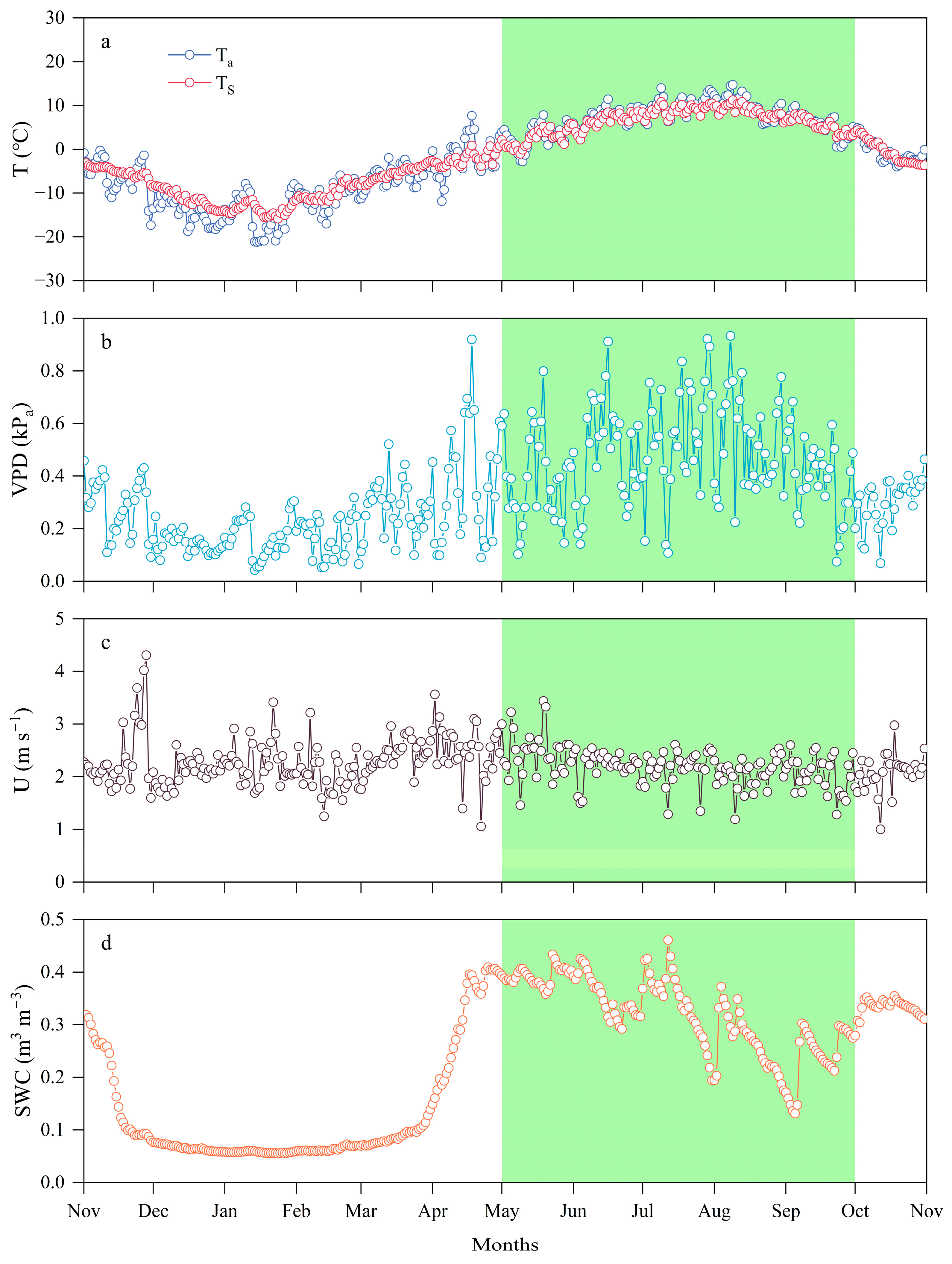
2.1. The Environmental Variables

Figure 1 shows the variation trends of environmental factors (Ta, Ts, VPD, U, and SWC) in the alpine meadow from 2022 to 2023, with specific data provided in Table 1. Throughout the vegetation growth period, the trends of Ta and Ts were similar, both reaching their minimum in January during the NGS, gradually increasing, peaking in July and August during the GS, and then gradually decreasing. During the cold NGS, VPD also decreases, reaching its minimum daily average in January, then gradually increasing and peaking during the warm and humid GS, with noticeable fluctuations in daily VPD. In contrast, U exhibits greater daily fluctuations during the NGS, whereas it remains more stable with smaller variations during the GS. The SWC is significantly influenced by air temperature throughout the vegetation growth period: It sharply declines starting in November, and from December to March, due to soil freezing, the daily average SWC remains low and stable. Starting in April, SWC rises rapidly, peaking during the GS, and then decreases again at the end of the GS.

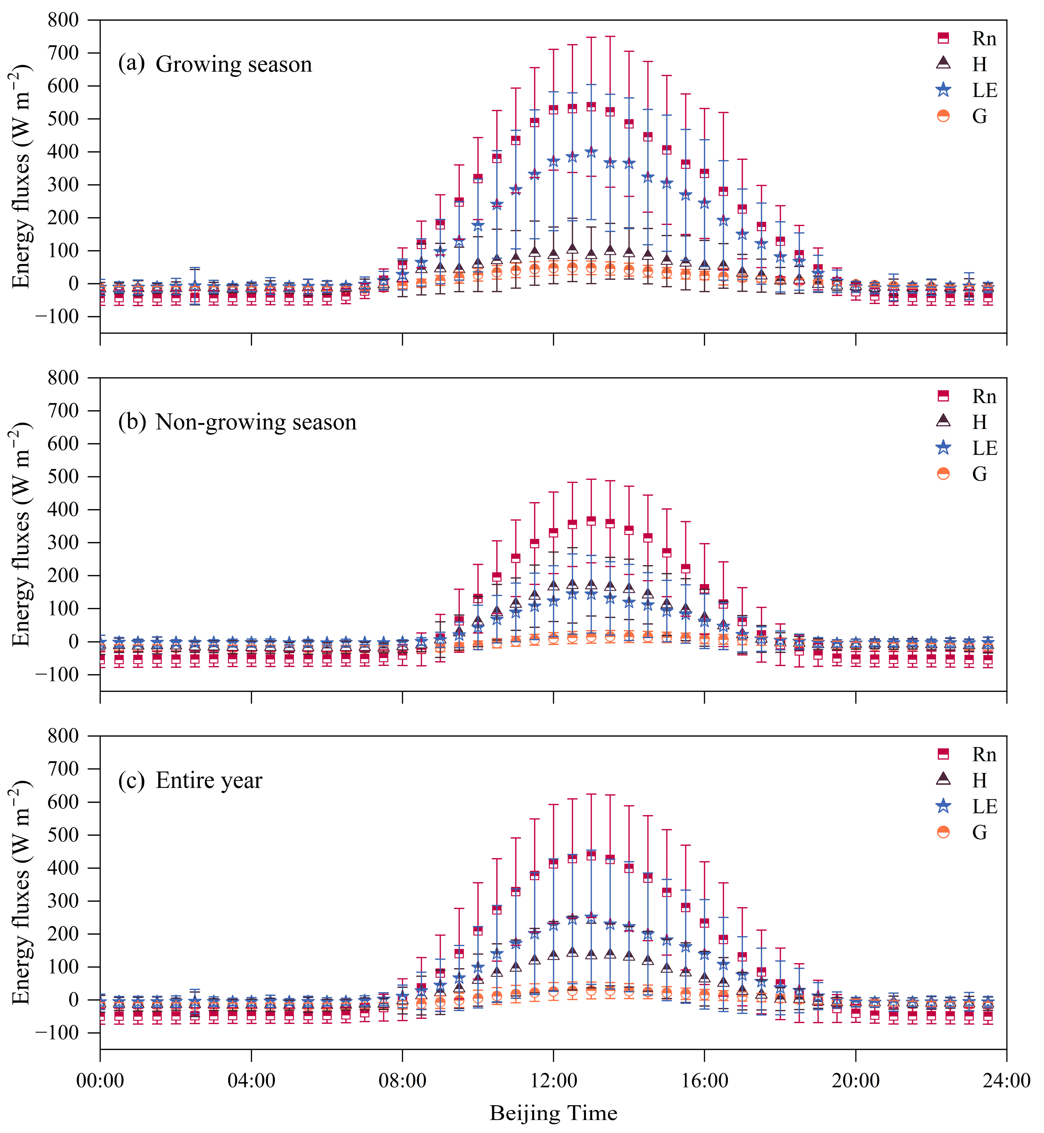
2.2. Daily Variations in the Characteristics of Energy

A paired t-test was performed on the half-hourly data of Rn, G, H, and LE during the GS and NGS. The results indicate significant differences in surface fluxes between the GS and NGS (** p < 0.01). Figure 2 illustrates the daily variation in energy fluxes in vegetation during the GS, NGS, and throughout the year. The daily variation trends of Rn, H, LE, and G display an n-shape, with Rn exhibiting the most pronounced and intense changes. The maximum peak typically occurs at 13:00, with an annual average of 437.4 W m−2. The peak during the GS is 536.94 W m−2, significantly higher than that of the NGS at 365.56 W m−2. Compared to other fluxes, the variation magnitude follows the order of LE > H > G, with the timing of the G peak being inconsistent. In the NGS, the peak occurs later, usually at 13:30 (15.95 W m−2), while during the GS, the peak is reached earlier at 12:30, being three times that of the NGS at 49.14 W m−2. The annual peak occurs at 13:00 (28.89 W m−2). Throughout the year, among the turbulent fluxes (H and LE), the overall average of LE is higher than that of H, and the timing of their peaks also differs. The annual daily average peak of H occurs at 12:30, measuring 142.27 W m−2, which is lower than the peak of LE (196.58 W m−2) and occurs half an hour earlier. During the GS, the peak of H occurs at 12:30 (102.67 W m−2), while the peak of LE occurs later at 13:00 (399.46 W m−2). In the NGS, the peak of H exceeds that of LE, both occurring at 12:30, measuring 170.84 W m−2 and 144.47 W m−2, respectively.

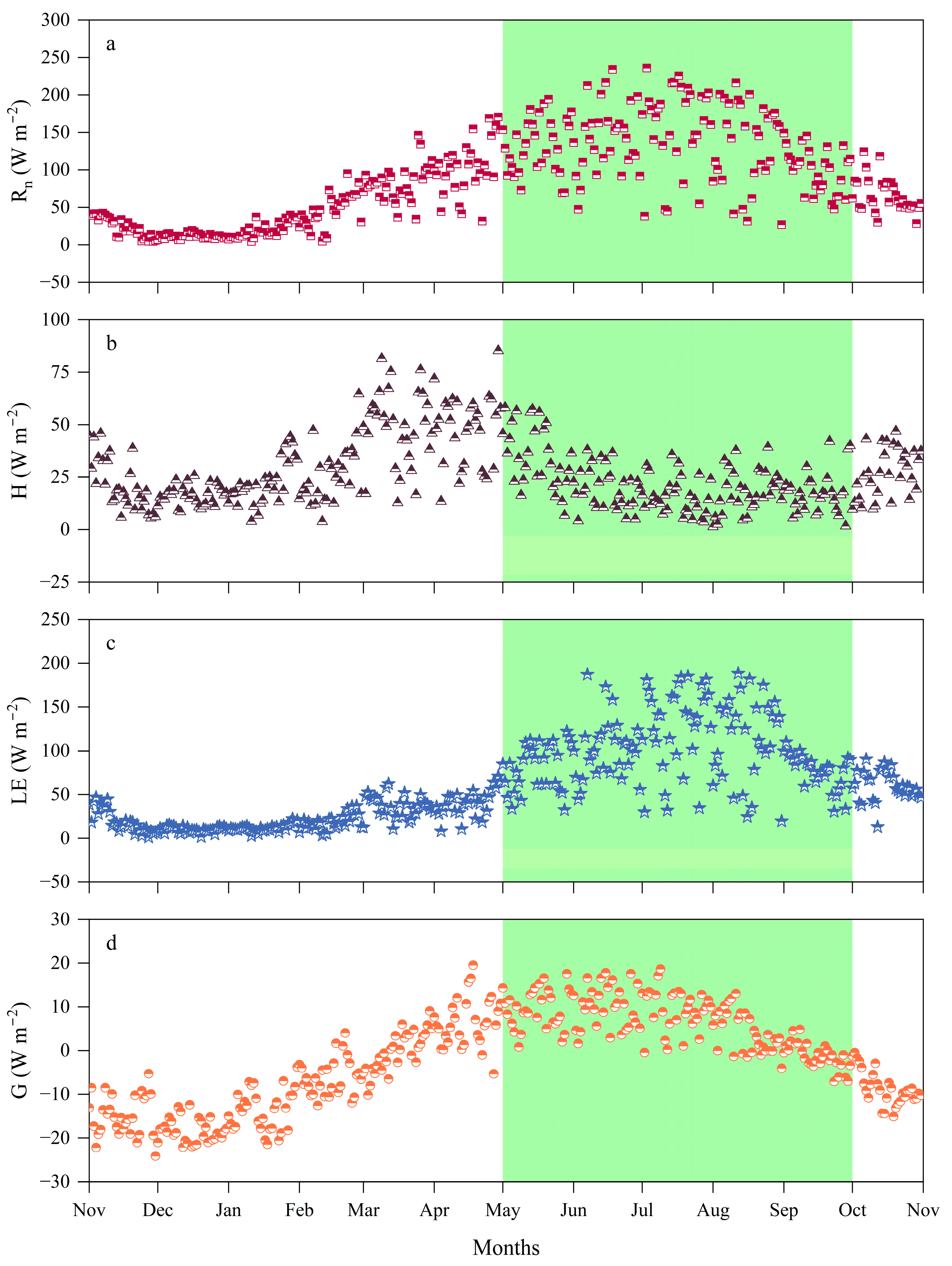
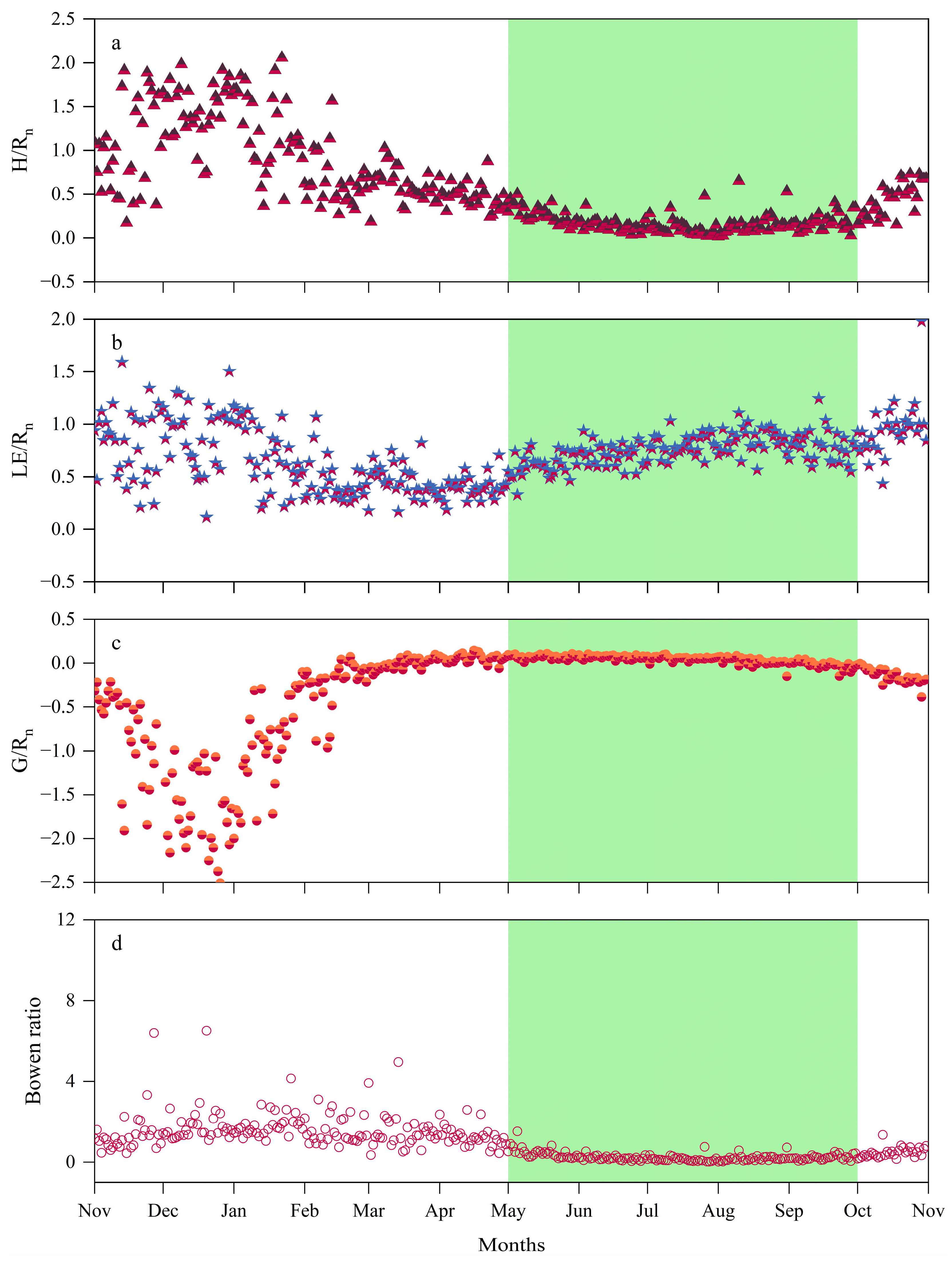
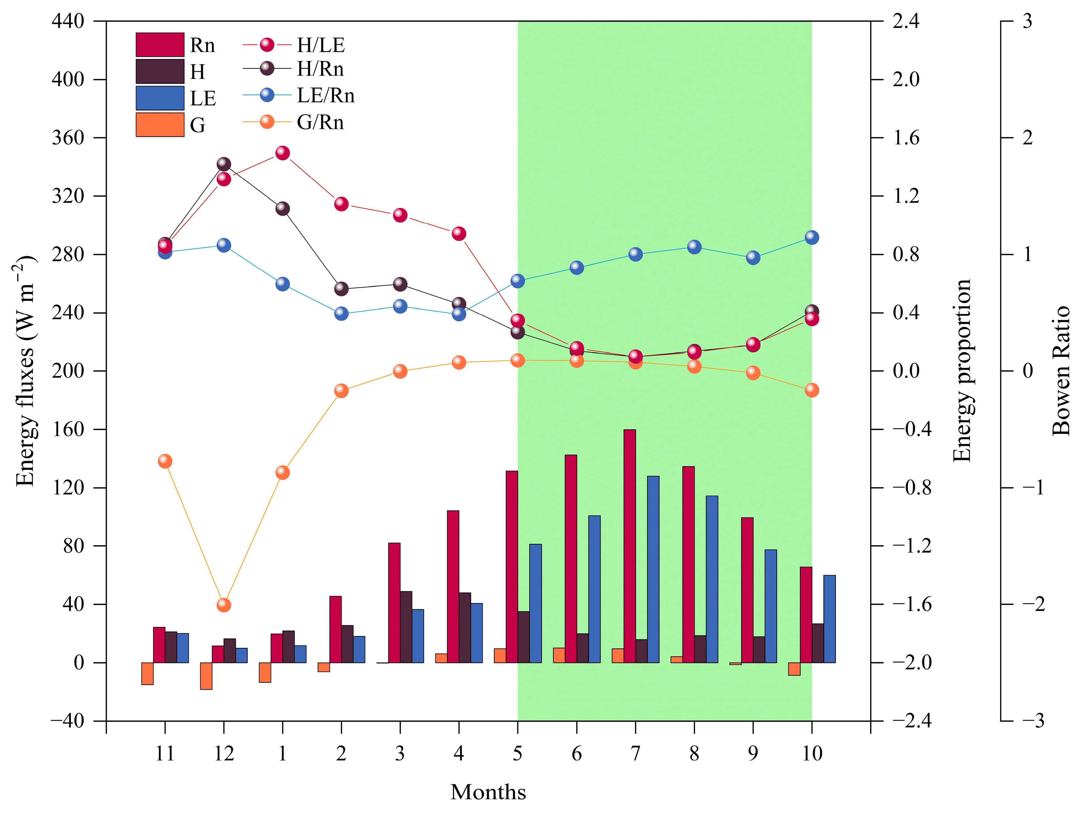
2.3. Seasonal Distribution and Proportional Characteristics of Energy Fluxes

Figure 3, Figure 4 and Figure 5 illustrate the trends and distribution characteristics of daily and monthly average values of surface energy components (Rn, H, LE, and G) in alpine meadows during the monitoring period, with the GS, NGS, and annual daily averages presented in Table 1. During the NGS, the daily average of Rn is relatively low due to the lower solar radiation angle and shorter daylight hours. In December, the monthly average of Rn reaches its minimum value of 11.46 W m−2, after which, Rn steadily increases. Once the GS begins, with longer daylight hours, the daily average substantially exceeds that of the NGS, peaking at 159.81 W m−2 in July, followed by a gradual decline.
The seasonal variation in LE follows a similar trend to Rn but the variations in H and LE differ substantially. In December, due to the lowest Rn and the lowest temperatures of the year, surface evaporation nearly halts, and the monthly averages of LE and H drop to 9.88 W m−2 and 15.26 W m−2, respectively. However, at this point, the H/Rn ratio exceeds the LE/Rn ratio. In January, the Bowen ratio reaches its highest value, with the Rn provided by solar radiation mainly converting to H. In March, the monthly average of H first reaches its peak (48.76 W m−2). By May, Rn undergoes significant changes, and the monthly average of LE exceeds that of H for the first time, causing the Bowen ratio to drop below 1. This indicates that, with increasing Rn, about two-thirds of the energy is converted into LE, while only one-third is transferred to the atmosphere as H. After entering the GS, with rapid vegetation growth and soil thawing, temperatures rise, and evaporation increases. LE peaks at 127.93 W m−2 in July, and then begins to decrease after August as Rn gradually declines. During this period, the LE/Rn ratio remains higher than the H/Rn ratio, and the Bowen ratio stays below 1, indicating that evaporation from vegetation and soil plays a dominant role in the energy distribution of Rn. Most of the Rn returns to the atmosphere in the form of LE. During this period, H decreases and stabilizes, with a slight increase in October. The seasonal variation in G is relatively stable, often negative during the NGS, indicating that soil heat is primarily transferred to the colder air. In December, the monthly average of G reaches its lowest value of the year (−18.41 W m−2). After that, G gradually increases and becomes positive in March. Entering the GS, G continues to rise and peaks in June at a monthly average of 10.02 W m−2, when the soil absorbs the continuously increasing Rn, and the G/Rn ratio reaches its highest value. Surface soil has slower thermal conductivity and limited heat exchange, so the G/Rn ratio remains consistently lower than both the H/Rn and LE/Rn ratios.

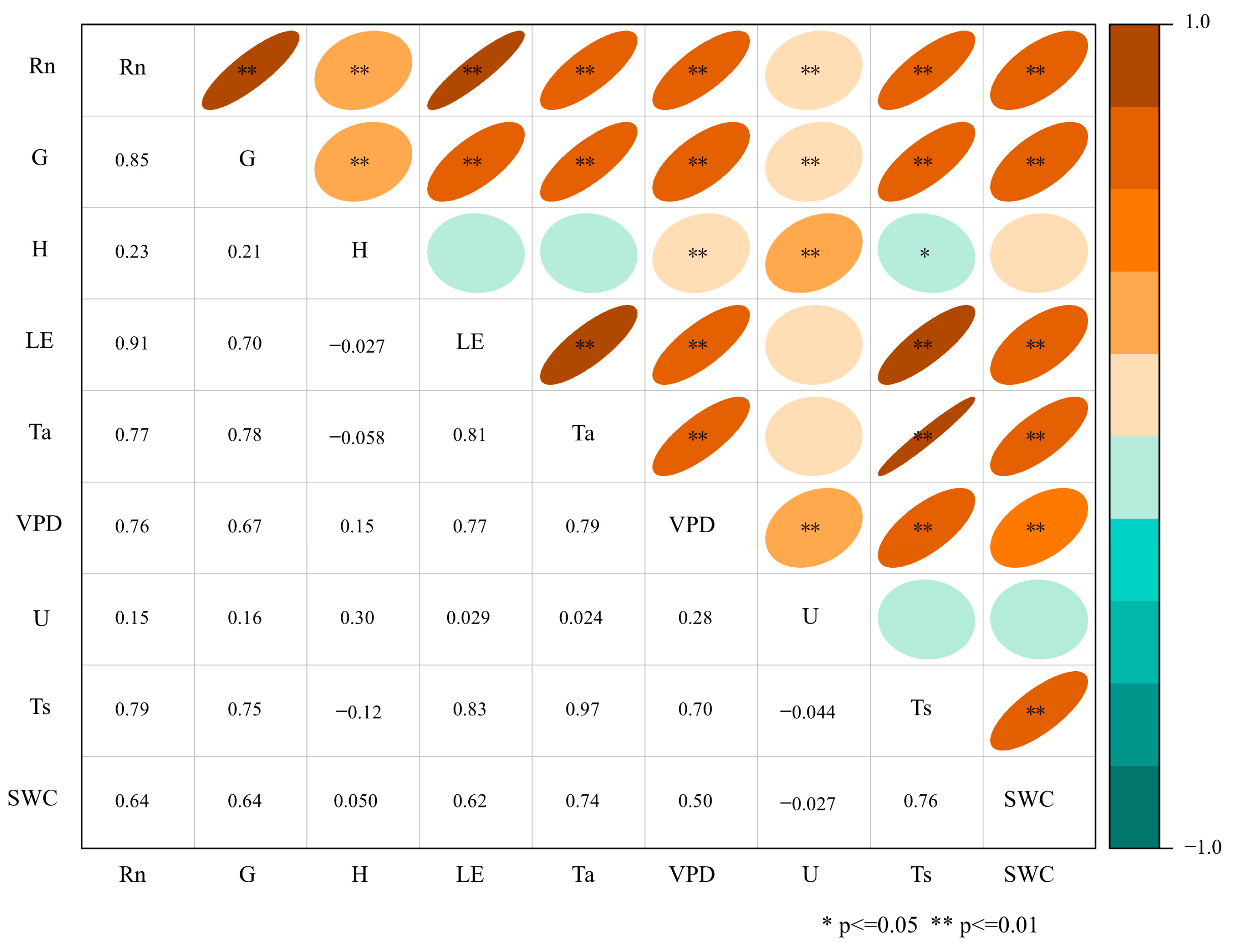
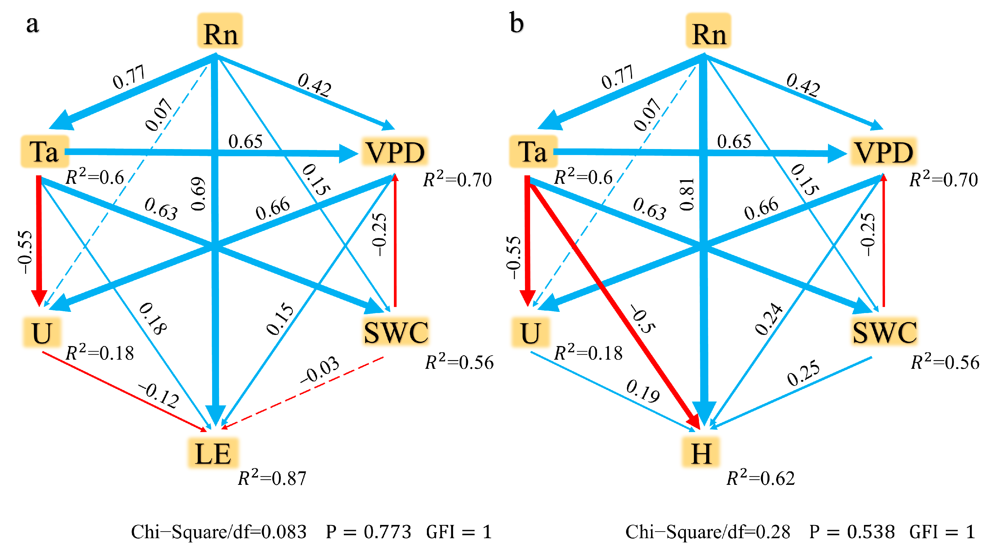
2.4. Factors Influencing Energy Fluxes

Figure 6 explores the relationship between meteorological variables (Rn, Ta, VPD, U, Ts, and SWC) and energy fluxes (H and LE) through Pearson’s correlation analysis. Based on the correlation results, a path analysis model was constructed in Figure 7 to analyze the direct and indirect effects of meteorological variables on H and LE.
The results of Pearson’s correlation analysis show that Rn is significantly positively correlated with both H and LE, indicating that Rn is the primary driving factor for both. The correlation between Ta and H is weak, indicating that changes in Ta have a less significant impact on H compared to LE. VPD is positively correlated with both H and LE, suggesting that under dry conditions, an increase in VPD enhances the flux of both. The correlation between U and H is small, while its correlation with LE is weak, indicating that U has a limited effect on energy fluxes. SWC shows a high positive correlation with LE but a lower correlation with H, indicating that wet soil conditions are more conducive to an increase in LE. Based on the results of Pearson’s correlation analysis, path analysis models for H and LE were constructed. During the model construction process, variables with higher correlation coefficients were prioritized as main pathways. Rn exhibited high correlations in both models, thus serving as the core driving factor in the path models. In the H model, the strong correlation between Ta and H led to Ta being included as a direct influencing factor. Although VPD has a relatively low correlation with H, its impact on air dryness allows it to be included as an indirect influencing variable in the model. U and SWC, having lower correlations with H, were given lower priority in the model. In the LE model, SWC shows the strongest correlation with LE, leading to its prioritization for inclusion, while U was also considered due to its promoting effect on evaporation and transpiration processes.
In the path analysis model for H, Rn has a significant direct effect on H, with a path coefficient of 0.81, indicating that Rn is the main driving factor for H. The path coefficient for Ta on H is −0.50, indicating a negative correlation between rising temperatures and H, suggesting that high-temperature conditions may suppress H. The path coefficient for VPD on H is 0.24, showing that in dry environments, the increase in VPD contributes relatively little to H. The path coefficient for U is 0.19, indicating that its effect on H is relatively small, yet it still contributes to energy exchange. The path coefficient for SWC is 0.25, indicating that H increases under moist soil conditions.
Rn also has a significant effect on LE, with a path coefficient of 0.69, emphasizing its core role in LE. The path coefficient for SWC on LE is −0.03, which is weak and not significant, while Ta has a path coefficient of 0.18, indicating a positive but limited effect on LE. The path coefficient for VPD on LE is 0.15, suggesting that an increase in VPD can promote the enhancement of LE. The path coefficient for U is −0.12, suggesting that an increase in U may have a negative impact on LE. The analysis results from the structural equation model clearly reveal the complex relationships of meteorological factors in the transmission of energy fluxes.

3. Discussion

3.1. Seasonal Variations in Energy Components

The three energy components, H, LE, and G, exhibit significant seasonal variations influenced by climate change and underlying surface conditions during the growth of vegetation in alpine meadows [42]. Comparing the results of this study with other research on alpine meadows in the QTP, it was found that the seasonal variation trends of surface energy fluxes (Rn, G, H, and LE) are consistent across different growth periods; however, differences in daily averages were observed. Compared to the western QTP regions of Xainza and Maqin, the daily averages of Rn and H are lower in this study area, with G values being similar, while LE is relatively higher [43,44]. In comparison to the central QTP regions of Zhiduo and Wudaoliang, Rn and LE are similar but G and H are relatively lower [45,46]. When compared with the eastern Qilian Mountains, particularly the Tianlaochi region, G and H are lower, while LE is higher, with Rn being significantly smaller [4]. The differences in Rn are likely influenced by factors such as elevation, topography, solar angles, and clear weather conditions [5,47]. The QTP region, with an elevation typically exceeding 4000 m, leads to higher Rn intensities at high altitudes. In the Tianlaochi region of the Qilian Mountains, Rn is relatively higher at the same elevation, while in the Arou region, Rn is similar [18]. The energy variation processes in our study area are weaker than in the QTP but similar to those in the Qilian Mountains. The Qilian Mountains are influenced by the monsoon earlier, resulting in a longer and more vigorous growing season. This causes an earlier shift in surface energy from H to LE [48,49].
The energy distribution during different growth periods is closely related to the state of meadow vegetation. During different time periods, either H or LE dominates the energy allocation. The distribution of LE and H in Rn significantly impacts local climate and hydrological processes [50]. The Bowen ratio (β, H/LE) serves as a key indicator of surface energy distribution [51]. During the NGS, as Rn decreases, H, LE, and G also decrease. Under conditions of snowfall and dry, cold temperatures, most of Rn is released to the atmosphere via H, making H the dominant energy flux and leading to β > 1. During this period, when the soil freezes, G typically has negative values, indicating that heat is being transferred from the soil to the cold air. Toward the end of the NGS, as Rn and Ta increase, H reaches its first peak in March–April, while the meadow begins to sprout and grow, leading to increases in LE and G. During the GS, Rn peaks in July, and G and LE reach their peaks slightly later in the month, trailing behind H. Currently, energy mainly returns to the atmosphere via evaporation from vegetation leaves and soil moisture, resulting in an increase in LE and a decrease in H, leading to β < 1. The soil absorbs a significant amount of heat from the atmosphere, and this heat reaches its peak during this period [52]. However, as the GS transitions into the NGS, Rn and Ta decrease, causing vegetation to wilt. As a result, transpiration declines, LE decreases, and H reaches a second minor peak. This regular variation in the surface energy components during vegetation growth in alpine meadows is also observed in other regions of the QTP [4,15,19,31,53].

3.2. Factors Influencing Energy Fluxes in Alpine Meadow Ecosystems

The path analysis model used in this study indicates that the primary factor influencing the surface turbulent flux in alpine meadows is Rn, which shows a significant positive correlation with surface turbulent fluxes. This relationship has been observed in numerous studies [18,54,55]. In addition to Rn, Ta is also a crucial factor affecting surface turbulence. The continuous increase in Rn requires a corresponding rise in Ta to maintain energy balance at the surface [56]. From the NGS to the GS, the increase in Rn causes a rise in Ta, leading to soil thawing, changes in soil bulk density, and a sharp increase in SWC, which in turn increases LE [57,58,59]. As the vegetation recovers from dormancy, the atmospheric humidity and VPD increase, further enhancing evaporation rates [60]. With vegetation growth, the leaf area expands, altering surface albedo and roughness, which further affects the distribution of turbulent fluxes through transpiration [59]. In April, the weakening of U balances the temperature difference, while the sharp rise in SWC promotes root water absorption, fostering plant growth. Increased photosynthesis and respiration enhance the absorption of Rn and its conversion to LE, leading to a decline in H and an increase in LE during this phase [45]. In the mid-GS, when Ta peaks, transpiration rates accelerate, causing LE to reach its maximum [61,62]. At this point, the higher vegetation coverage reduces albedo and inhibits the soil temperature rise, leading to a decrease in H [63]. The intense evaporation processes from vegetation and the moist soil surface contribute to the peak in LE [64]. The increase in LE corresponds to climate warming and reflects the growing phenomenon of shrubification in the alpine meadows at the study site. Excessively high Ta, along with VPD, can cause plants to close their stomata as a self-protective measure, thus reducing photosynthesis and transpiration rates [65]. An increase in SWC also limits root absorption of moisture, further decreasing evaporation rates [66]. The longer duration of LE dominance during the GS shortens the soil freezing and thawing period, and an increased SWC leads to more extensive melting of the frozen soil layer, releasing more heavy metals, which contribute to meadow degradation [67]. The impact of precipitation at different stages on surface turbulence is also noteworthy. During the NGS, precipitation is limited but snowfalls are frequent. The melting of snow and the formation of new snow temporarily affect LE, leading to its increase. The high albedo of accumulated snow reflects more Lu, thereby reducing Rn [68]. During this snowmelt process, significant and unstable daily fluctuations in the H/Rn and LE/Rn ratios are observed in the NGS. In contrast, during the GS, precipitation is primarily in the form of rainfall. During the rainy season, SWC is generally higher than in the dry season [69]. Rainfall increases the water vapor content in the atmosphere, which enhances plant growth and leads to an increase in evapotranspiration, causing LE to peak [35,70]. In the GS, vegetation gradually increases its leaf area, continuously changing surface albedo and roughness, which further affect the distribution of turbulent fluxes through transpiration [59]. During the early GS, the expanding leaf area of vegetation reduces the soil reflection of Rn, which in turn reduces the temperature difference between the atmosphere and surface, lowering H [63]. In the mid-GS, the combined processes of intense photosynthesis, respiration, and soil evaporation from moist surfaces drive LE to its peak [64].
Nevertheless, this study has certain limitations. During surface flux studies in alpine meadows, an energy imbalance is often observed [28]. The BREB, based on the Kh = Kv assumption, is a simplified model for studying surface flux variations and requires strict meteorological conditions. The accuracy of the experimental instruments, atmospheric instability, and the use of roughness parameters derived from similar regions also impact the results, leading to an energy imbalance. Additionally, other influencing factors, such as atmospheric cloud cover variations during different growth periods, were not considered and may affect direct solar radiation reaching the surface. The study area has a long snow-covered period, and a lack of records on snowmelt reduces the accuracy of LE calculations during the NGS. The absence of surface albedo references for different seasons, along with the lack of records for the vegetation leaf area index or specific dates of growth and dormancy, also affects the study of surface flux variations in alpine meadows.

4. Materials and Methods
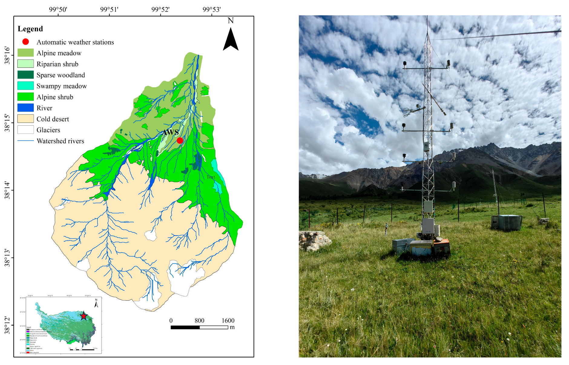
4.1. Study Site

This study was conducted in the Hulu catchment of the upper Heihe River basin in the QTP (latitude 38°12′–38°17′, longitude 99°50′–99°54′; see Figure 8) [71]. The elevation of the catchment ranges from 2960 to 4820 m, covering an area of 23.1 km2 [72]. The catchment exhibits distinct alpine mountain climatic characteristics, with a climate type classified as continental and cold humid. Temperatures are low and highly variable, with precipitation occurring concurrently with temperature changes. The annual average daily temperature and precipitation recorded by the National Meteorological Station from 2022 to 2023 were 0.86 °C and 436.02 mm, respectively. Precipitation is primarily concentrated in the warm and humid growing season (from May to September), accounting for 88% of the annual total, while the remaining months (from October to April) are characterized by dry and cold conditions. The main vegetation and corresponding soil types in the catchment include the following: the alpine meadow community was dominated by Carex myosuroides Vill., with the surface soil classified as Mollisols. The riparian shrub community was characterized by Hippophae tibetana Schltdl., with the underlying soil classified as Inceptisols. The sparse woodland community consisted of Picea crassifolia Kom. and Juniperus przewalskii Kom., with soils primarily classified as Inceptisols and Mollisols. The swampy meadow community was dominated by Blysmus compressus (L.) Panz. Ex Link, with the soil classified as Histosols. The alpine shrub community had species such as Dasiphora fruticosa (L.) Rydb. and Caragana jubata (Pall.) Poir., where the soils are a combination of Inceptisols and Entisols. The cold desert community was characterized by Rhodiola rosea L., with Gelisols as the predominant soil type [36].

4.2. Instruments and Measurements

We selected the meteorological observation station in the central alpine meadow of the Hulu catchment (38°24.9′ N, 99°87.4′ E), at an elevation of 3232 m. The observation area is a flat, open valley bottom, approximately 400 m from the mountain, with a slope of less than 10°. A 10 m × 10 m fenced area was established around the station to ensure the safety and stable operation of the equipment. Vegetation information at the study site was determined using sampling methods. The dominant vegetation was K. myosuroides, with the accompanying plant C. moorcroftii. During the GS (May to September), the vegetation cover is approximately 92%, with an average height of about 0.25 m. In the NGS (October to April of the following year), the average height of the vegetation is about 0.15 m.
An integrated environmental monitoring system was installed at the experimental site, including a four-component radiation sensor and a soil temperature sensor to collect data on different solar radiation components and surface air temperature. Air temperature and humidity sensors, as well as a wind speed sensor, were installed at two different heights. Soil sensors were placed at various soil depths, including soil temperature sensors, soil moisture sensors, and soil heat flux sensors. Detailed information on all sensors is provided in Table 2. All measured data were averaged over 30-minute intervals and stored using a data logger (CR1000, Campbell Scientific, Logan, UT, USA) set up at the experimental station. The system collected observational data from 1 November 2022 to 31 October 2023.

4.3. Bowen Ratio Energy Balance (BREB) Method

In this study, we used the BREB method to calculate surface energy changes. This method is well-established, reliable, and widely applied in numerous studies of surface energy variations [43]. According to the first law of thermodynamics, solar radiation entering the surface is absorbed and reflected. Equation (1) represents the mathematical formulation for surface energy balance:
R n = G + H + L E + S
Equation (2) calculates Rn using data collected by the radiation instruments set up in the integrated environmental monitoring system:
R n = S d S u + L d L u
Equation (3) calculates G using embedded soil heat flux plates and temperature gradients at different soil depths:
G = G P + C s z T t
where S represents the energy produced by leaf metabolism and storage (W·m−2), which are usually neglected in calculations. In 1926, the Bowen ratio was proposed as the ratio of H to LE, assuming that the exchange coefficients for water vapor and heat between two horizontal planes perpendicular to the evaporation direction are similar, i.e., Kh = Kv. The corresponding mathematical equation is presented in Equation (4), outlined below:
β = H L E = ρ a C p K h T 2 T 1 + τ ( Z 2 Z 1 ) ρ a C p K w ( e 2 e 1 ) / γ = γ T 2 T 1 + τ ( Z 2 Z 1 ) e 2 e 1
To reduce errors, Foken et al. (2008) recommended that temperature and humidity be measured at two heights, with a height ratio of 4–8 [73]. In this study, Z1 and Z2 were chosen as 0.15 m and 7.70 m, respectively. Using Equations (1) and (4), we can calculate the H and LE as follows:
L E = R n G ( 1 + β )
H = β ( R n G ) ( 1 + β )
All abbreviations are shown in Table 3.

4.4. Exclusion of Outliers and Imputation

The results of the BREB model assume that Kh = Kv, which requires the underlying surface to be homogeneous. According to the turbulent flux footprint model proposed by Hsieh et al. (2000) [74], the 90% fetch-to-measurement height ratio is 54 m. Considering that the heights of the two humidity and temperature sensors are 1.5 m and 7.7 m, respectively, their geometric mean is 3.4 m. This indicates that 90% of the effective turbulent flux is confined within a radius of 184 m from the meteorological tower. Meanwhile, the homogeneity of the experimental area is sufficiently stable, making the results obtained from the BREB model reasonable.
To obtain continuously recorded data, this study utilized linear interpolation and the average diurnal variation method to fill in missing meteorological data caused by extreme weather and instrument failures [75]. After data processing and imputation of missing values, the data were further aggregated into daily averages. When using the BREB method to calculate surface fluxes, turbulence data obtained during the morning and evening are often unreliable.
To ensure the reliability of the results obtained using the BREB method, quality control was implemented based on the dynamic error exclusion standard (β) proposed by Hu et al. (2014), which is based on the typical instrument resolution. The following quality control criterion was applied to the computed data [76]:
1 δ 1 γ δ 2 e < β < 1 + δ 1 γ δ 2 e
This screening process ensures the accuracy of the turbulent flux calculations. For missing data in the BREB method, the flux profile method was used for calculation and imputation [45].

4.5. Energy Closure Calculation

Due to the prevalent energy imbalance in alpine meadows [19,77], it is necessary to verify the reliability of daily averaged energy values on the surface. The energy closure ratio (EBR) typically ranges from 0.55 to 0.99. To validate this, we used the energy closure calculation formula (Equation (8)) and performed linear regression between the available energy and turbulent flux:
E B R = ( H + L E ) ( R n G )
The energy balance closure ratio (EBR) was calculated to be 0.85. As shown in Figure 9, the slope of the linear regression was 0.92, indicating a strong correlation between turbulent flux and available energy. This suggests that the calculated turbulence data are reliable [18,78].

4.6. Data Analysis

The surface fluxes of Rn, G, H, and LE exhibit significant differences between the GS and NGS. To assess these differences, a paired t-test was conducted on the half-hourly data. To determine the relationship between H and LE and their potential influencing factors (Ta, Ts, U, VPD, Rn, SWC), we conducted Pearson’s correlation analysis to assess the strength and direction of linear relationships between these variables. Simultaneously, a Pearson correlation heatmap was generated using Origin software (OriginLab Corporation, Northampton, MA, USA), version 2024. The heatmap visually represents the correlation coefficients between variables, with * p < 0.05 and ** p < 0.01 indicating significant and highly significant relationships, respectively (see Figure 6). Based on the results of Pearson’s correlation analysis, path analysis models for H and LE were constructed. Path analysis allowed us to quantify the direct and indirect effects of the meteorological factors on H and LE, providing a comprehensive understanding of the energy flux dynamics. We utilized the Goodness of Fit Index (GFI) and Chi-Square/df ratio to evaluate the performance and adequacy of the path analysis model. The model was considered well-constructed if the Goodness of Fit Index (GFI) was greater than 0.9 and the Chi-Square/df ratio was less than 3. All statistical analyses were conducted using the SPSS Amos 22.0 platform (IBM Inc., Armonk, NY, USA) [79].

5. Conclusions

This study collected meteorological data during the growth process of an alpine meadow and applied the BREB model to calculate the surface energy balance. This study focuses on analyzing the variations, proportions, and influencing factors of surface fluxes during different time periods. The results show that the daily peak values of surface fluxes occur around 1:00 PM, with lower values in the growing season (GS) compared to the non-growing season (NGS). Although the trends are consistent, there are significant differences in the magnitudes of the variations. On an annual scale, the LE/Rn ratio is higher than the H/Rn ratio, and G occupies the smallest proportion throughout the year, with most Rn being returned to the atmosphere as LE. Specifically, in the growing season, Rn is primarily converted to H, while in the non-growing season, it is mainly converted to LE. The path analysis and Pearson’s correlation analysis both indicate that Rn is the primary driver of both LE and H, followed by Ta, which has a stronger effect on H than on LE. VPD and SWC have a stronger impact on LE than on H, while U has a limited influence on surface fluxes. Overall, this study provides foundational data on the climate response of alpine meadows; however, the observation period was relatively short, and future research could benefit from using remote-sensing data to track long-term vegetation growth changes over a wider area, with an emphasis on the impact of extreme weather on the energy balance and the feedback mechanisms between vegetation growth and energy fluxes.

Author Contributions

Conceptualization, Y.T., Y.F. and Z.L.; Data curation, Y.L., H.T., and C.H.; Formal analysis, Y.T. and X.A.; Funding acquisition, Y.F., Z.L. and C.H.; Investigation, Y.T., Z.L., Y.L. and H.T.; Methodology, Y.T., Y.F. and Z.L.; Project administration, Z.L.; Resources, Z.L.; Software, Y.T.; Supervision, Z.L. and R.C.; Visualization, Y.T. and Y.F.; Writing—original draft, Y.T.; Writing—review and editing, Y.T. and Z.L. All authors have read and agreed to the published version of the manuscript.

Funding

This study was funded by the National Natural Sciences Foundation of China (42171147 and 52369007), Inter-Institute Youth United Fund of Lanzhou Branch, Chinese Academy of Sciences, 2024-LZFYQNLHJJ-02.

Data Availability Statement

Data will be made available on request.

Conflicts of Interest

The authors declare no conflicts of interest.

References

  1. Qu, S.; Xu, R.; Yu, J.; Li, F.; Wei, D.; Borjigidai, A. Nitrogen deposition accelerates greenhouse gas emissions at an alpine steppe site on the Tibetan Plateau. Sci. Total Environ. 2021, 765, 144277. [Google Scholar] [CrossRef] [PubMed]
  2. Si, M.; Guo, X.; Lan, Y.; Fan, B.; Cao, G. Effects of Climatic Variability on Soil Water Content in an Alpine Kobresia Meadow, Northern Qinghai–Tibetan Plateau, China. Water 2022, 14, 2754. [Google Scholar] [CrossRef]
  3. Aires, L.M.; Pio, C.A.; Pereira, J.S. The effect of drought on energy and water vapour exchange above a mediterranean C3/C4 grassland in Southern Portugal. Agric. For. Meteorol. 2008, 148, 565–579. [Google Scholar] [CrossRef]
  4. Gao, Y.; Zhao, C.; Rong, Z.; Liu, J.; Wang, Q.; Ge, L.; Guo, Z.; Mao, Y. Energy exchange between the atmosphere and a subalpine meadow in the Qilian Mountains, northwest China. J. Hydrol. 2019, 572, 771–780. [Google Scholar]
  5. Iziomon, M.G.; Mayer, H. On the variability and modelling of surface albedo and long-wave radiation components. Agric. For. Meteorol. 2002, 111, 141–152. [Google Scholar] [CrossRef]
  6. Wang, Y.; You, C.; Gao, Y.; Li, Y.; Niu, Y.; Shao, C.; Wang, X.; Xin, X.; Yu, G.; Han, X.; et al. Seasonal variations and drivers of energy fluxes and partitioning along an aridity gradient in temperate grasslands of Northern China. Agric. For. Meteorol. 2023, 342, 109736. [Google Scholar] [CrossRef]
  7. Yue, P.; Zhang, Q.; Zhang, L.; Li, H.; Yang, Y.; Zeng, J.; Wang, S. Long-term variations in energy partitioning and evapotranspiration in a semiarid grassland in the Loess Plateau of China. Agric. For. Meteorol. 2019, 278, 323–336. [Google Scholar] [CrossRef]
  8. Zhang, K.; Liu, D.; Liu, H.; Lei, H.; Guo, F.; Xie, S.; Meng, X.; Huang, Q. Energy flux observation in a shrub ecosystem of a gully region of the Chinese Loess Plateau. Ecohydrol. Hydrobiol. 2022, 22, 323–336. [Google Scholar] [CrossRef]
  9. Liu, X.; Chen, B. Climatic warming in the Tibetan Plateau during recent decades. Int. J. Climatol. 2000, 20, 1729–1742. [Google Scholar] [CrossRef]
  10. Zhang, L.; Shen, M.; Yang, Z.; Wang, Y.; Chen, J. Spatial variations in the difference in elevational shifts between greenness and temperature isolines across the Tibetan Plateau grasslands under warming. Sci. Total Environ. 2024, 906, 167715. [Google Scholar] [CrossRef]
  11. Ma, Y.; Guan, Q.; Sun, Y.; Zhang, J.; Yang, L.; Yang, E.; Li, H.; Du, Q. Three-dimensional dynamic characteristics of vegetation and its response to climatic factors in the Qilian Mountains. Catena 2022, 208, 105694. [Google Scholar] [CrossRef]
  12. Qian, D.; Du, Y.; Li, Q.; Guo, X.; Fan, B.; Cao, G. Impacts of alpine shrub-meadow degradation on its ecosystem services and spatial patterns in Qinghai-Tibetan Plateau. Ecol. Indic. 2022, 135, 108541. [Google Scholar] [CrossRef]
  13. Wei, L.; Zhao, W.; Feng, X.; Han, C.; Li, T.; Qi, J.; Li, Y. Freeze-thaw desertification of alpine meadow in Qilian Mountains and the implications for alpine ecosystem management. Catena 2023, 232, 107471. [Google Scholar] [CrossRef]
  14. Zhang, L.; Chen, Z.; Zhang, X.; Zhao, L.; Li, Q.; Chen, D.; Tang, Y.; Gu, S. Evapotranspiration and Its Partitioning in Alpine Meadow of Three-River Source Region on the Qinghai-Tibetan Plateau. Water 2021, 13, 2061. [Google Scholar] [CrossRef]
  15. Chen, S.P.; Chen, J.Q.; Lin, G.H.; Zhang, W.L.; Miao, H.X.; Wei, L.; Huang, J.H.; Han, X.G. Energy balance and partition in Inner Mongolia steppe ecosystems with different land use types. Agric. For. Meteorol. 2009, 149, 1800–1809. [Google Scholar] [CrossRef]
  16. Ryu, Y.; Baldocchi, D.D.; Ma, S.; Hehn, T. Interannual variability of evapotranspiration and energy exchange over an annual grassland in California. J. Geophys. Res. Atmos. 2008, 113, D09104. [Google Scholar] [CrossRef]
  17. Yan, C.; Zhao, W.; Wang, Y.; Yang, Q.; Zhang, Q.; Qiu, G.Y. Effects of forest evapotranspiration on soil water budget and energy flux partitioning in a subalpine valley of China. Agric. For. Meteorol. 2017, 246, 207–217. [Google Scholar] [CrossRef]
  18. Chang, Y.P.; Ding, Y.J.; Zhang, S.Q.; Qin, J.; Zhao, Q.D. Dynamics and environmental controls of evapotranspiration for typical alpine meadow in the northeastern Tibetan Plateau. J. Hydrol. 2022, 612, 128282. [Google Scholar] [CrossRef]
  19. Gu, S.; Tang, Y.; Cui, X.; Kato, T.; Du, M.; Li, Y.; Zhao, X. Energy exchange between the atmosphere and a meadow ecosystem on the Qinghai–Tibetan Plateau. Agric. For. Meteorol. 2005, 129, 175–185. [Google Scholar] [CrossRef]
  20. Hu, Z.; Wang, G.; Sun, X.; Huang, K.; Song, C.; Li, Y.; Sun, S.; Sun, J.; Lin, S.; Zhang, Y. Energy partitioning and controlling factors of evapotranspiration in an alpine meadow in the permafrost region of the Qinghai-Tibet Plateau. J. Plant Ecol. 2024, 17, rtae002. [Google Scholar] [CrossRef]
  21. Li, J.; Jiang, S.; Wang, B.; Jiang, W.-W.; Tang, Y.-H.; Du, M.-Y.; Gu, S. Evapotranspiration and Its Energy Exchange in Alpine Meadow Ecosystem on the Qinghai-Tibetan Plateau. J. Integr. Agric. 2013, 12, 1396–1401. [Google Scholar] [CrossRef]
  22. Li, Y.; Sun, R.; Liu, S. Vegetation physiological parameter setting in the Simple Biosphere model 2 (SiB2) for alpine meadows in the upper reaches of Heihe river. Sci. China Earth Sci. 2014, 58, 755–769. [Google Scholar] [CrossRef]
  23. Shang, L.Y.; Zhang, Y.; Lü, S.H.; Wang, S.Y. Energy exchange of an alpine grassland on the eastern Qinghai-Tibetan Plateau. Sci. Bull. 2015, 60, 435–446. [Google Scholar] [CrossRef]
  24. Xie, J.; Yu, Y.; Li, J.-l.; Ge, J.; Liu, C. Comparison of surface sensible and latent heat fluxes over the Tibetan Plateau from reanalysis and observations. Meteorol. Atmos. Phys. 2018, 131, 567–584. [Google Scholar] [CrossRef]
  25. Yang, K.; Guo, X.; Wu, B. Recent trends in surface sensible heat flux on the Tibetan Plateau. Sci. China Earth Sci. 2010, 54, 19–28. [Google Scholar] [CrossRef]
  26. Ma, Y.; Fan, S.; Ishikawa, H.; Tsukamoto, O.; Yao, T.; Koike, T.; Zuo, H.; Hu, Z.; Su, Z. Diurnal and inter-monthly variation of land surface heat fluxes over the central Tibetan Plateau area. Theor. Appl. Climatol. 2004, 80, 259–273. [Google Scholar] [CrossRef]
  27. Wang, S.; Ma, Y.; Liu, Y. Simulation of sensible and latent heat fluxes on the Tibetan Plateau from 1981 to 2018. Atmos. Res. 2022, 271, 106129. [Google Scholar] [CrossRef]
  28. Xin, Y.-F.; Chen, F.; Zhao, P.; Barlage, M.; Blanken, P.; Chen, Y.-L.; Chen, B.; Wang, Y.-J. Surface energy balance closure at ten sites over the Tibetan plateau. Agric. For. Meteorol. 2018, 259, 317–328. [Google Scholar] [CrossRef]
  29. Yao, J.; Zhao, L.; Ding, Y.; Gu, L.; Jiao, K.; Qiao, Y.; Wang, Y. The surface energy budget and evapotranspiration in the Tanggula region on the Tibetan Plateau. Cold Reg. Sci. Technol. 2008, 52, 326–340. [Google Scholar] [CrossRef]
  30. Yao, J.M.; Zhao, L.; Gu, L.L.; Qiao, Y.P.; Jiao, K.Q. The surface energy budget in the permafrost region of the Tibetan Plateau. Atmos. Res. 2011, 102, 394–407. [Google Scholar] [CrossRef]
  31. Zhang, S.Y.; Li, X.Y.; Zhao, G.Q.; Huang, Y.M. Surface energy fluxes and controls of evapotranspiration in three alpine ecosystems of Qinghai Lake watershed, NE Qinghai-Tibet Plateau. Ecohydrology 2015, 9, 267–279. [Google Scholar] [CrossRef]
  32. Ma, Y.; Yao, T.; Zhong, L.; Wang, B.; Xu, X.; Hu, Z.; Ma, W.; Sun, F.; Han, C.; Li, M.; et al. Comprehensive study of energy and water exchange over the Tibetan Plateau: A review and perspective: From GAME/Tibet and CAMP/Tibet to TORP, TPEORP, and TPEITORP. Earth-Sci. Rev. 2023, 237, 104312. [Google Scholar] [CrossRef]
  33. Zhang, X.; Gu, S.; Zhao, X.; Cui, X.; Zhao, L.; Xu, S.; Du, M.; Jiang, S.; Gao, Y.; Ma, C.; et al. Radiation partitioning and its relation to environmental factors above a meadow ecosystem on the Qinghai-Tibetan Plateau. J. Geophys. Res. Atmos. 2010, 115, D10106. [Google Scholar] [CrossRef]
  34. Tanaka, K.; Ishikawa, H.; Hayashi, T.; Tamagawa, I.; Ma, Y. Surface Energy Budget at Amdo on the Tibetan Plateau using GAME/Tibet IOP98 Data. J. Meteorol. Soc. Jpn. Ser. II 2001, 79, 505–517. [Google Scholar] [CrossRef]
  35. Li, H.Q.; Zhang, F.W.; Zhu, J.B.; Guo, X.W.; Li, Y.K.; Lin, L.; Zhang, L.M.; Yang, Y.S.; Li, Y.N.; Cao, G.M.; et al. Precipitation rather than evapotranspiration determines the warm-season water supply in an alpine shrub and an alpine meadow. Agric. For. Meteorol. 2021, 300, 108318. [Google Scholar] [CrossRef]
  36. Liu, Z.; Chen, R.; Qi, J.; Dang, Z.; Han, C.; Yang, Y. Control of Mosses on Water Flux in an Alpine Shrub Site on the Qilian Mountains, Northwest China. Plants 2022, 11, 3111. [Google Scholar] [CrossRef]
  37. Lu, H.; Koike, T.; Yang, K.; Hu, Z.; Xu, X.; Rasmy, M.; Kuria, D.; Tamagawa, K. Improving land surface soil moisture and energy flux simulations over the Tibetan plateau by the assimilation of the microwave remote sensing data and the GCM output into a land surface model. Int. J. Appl. Earth Obs. Geoinf. 2012, 17, 43–54. [Google Scholar] [CrossRef]
  38. Byun, K.; Liaqat, U.W.; Choi, M. Dual-model approaches for evapotranspiration analyses over homo- and heterogeneous land surface conditions. Agric. For. Meteorol. 2014, 197, 169–187. [Google Scholar] [CrossRef]
  39. Escarabajal-Henarejos, D.; Fernández-Pacheco, D.G.; Molina-Martínez, J.M.; Martínez-Molina, L.; Ruiz-Canales, A. Selection of device to determine temperature gradients for estimating evapotranspiration using energy balance method. Agric. Water Manag. 2015, 151, 136–147. [Google Scholar] [CrossRef]
  40. Zhuang, Y.; Zhao, W. Dew formation and its variation in Haloxylon ammodendron plantations at the edge of a desert oasis, northwestern China. Agric. For. Meteorol. 2017, 247, 541–550. [Google Scholar] [CrossRef]
  41. Li, H.; Zhang, F.; Zhu, J.; Li, J.; Guo, X.; Zhou, H.; Li, Y. Surface Albedo Dominates Radiation Efficiency of Alpine Grasslands Along an Elevation Profile of Qilian Mountains. J. Geophys. Res. Atmos. 2024, 129, e2023JD040649. [Google Scholar] [CrossRef]
  42. Minderlein, S.; Menzel, L. Evapotranspiration and energy balance dynamics of a semi-arid mountainous steppe and shrubland site in Northern Mongolia. Environ. Earth Sci. 2014, 73, 593–609. [Google Scholar] [CrossRef]
  43. Wang, K.; Ma, N.; Zhang, Y.; Qiang, Y.; Guo, Y. Evapotranspiration and energy partitioning of a typical alpine wetland in the central Tibetan Plateau. Atmos. Res. 2022, 267, 105931. [Google Scholar] [CrossRef]
  44. Zhang, X.; Liu, X.; Zhang, L.; Chen, Z.; Zhao, L.; Li, Q.; Chen, D.; Gu, S.J.A.; Meteorology, F. Comparison of energy partitioning between artificial pasture and degraded meadow in three-river source region on the Qinghai-Tibetan Plateau: A case study. Environ. Earth Sci. 2019, 271, 251–263. [Google Scholar] [CrossRef]
  45. You, Q.G.; Xue, X.; Peng, F.; Dong, S.Y.; Gao, Y.H. Surface water and heat exchange comparison between alpine meadow and bare land in a permafrost region of the Tibetan Plateau. Agric. For. Meteorol. 2017, 232, 48–65. [Google Scholar] [CrossRef]
  46. Peng, F.; You, Q.; Xue, X.; Guo, J.; Wang, T.J.E.E. Evapotranspiration and its source components change under experimental warming in alpine meadow ecosystem on the Qinghai-Tibet plateau. Ecol. Eng. 2015, 84, 653–659. [Google Scholar] [CrossRef]
  47. Allen, R.G.; Trezza, R.; Tasumi, M. Analytical integrated functions for daily solar radiation on slopes. Agric. For. Meteorol. 2006, 139, 55–73. [Google Scholar] [CrossRef]
  48. Ma, Y.; Wang, Y.; Wu, R.; Hu, Z.; Yang, K.; Li, M.; Ma, W.; Zhong, L.; Sun, F.; Chen, X.; et al. Recent advances on the study of atmosphere-land interaction observations on the Tibetan Plateau. Hydrol. Earth Syst. Sci. 2009, 13, 1103–1111. [Google Scholar] [CrossRef]
  49. Tanaka, K.; Tamagawa, I.; Ishikawa, H.; Ma, Y.M.; Hu, Z.Y. Surface energy budget and closure of the eastern Tibetan Plateau during the GAME-Tibet IOP 1998. J. Hydrol. 2003, 283, 169–183. [Google Scholar] [CrossRef]
  50. Mu, Y.M.; Yuan, Y.; Jia, X.; Zha, T.S.; Qin, S.G.; Ye, Z.Q.; Liu, P.; Yang, R.Z.; Tian, Y. Hydrological losses and soil moisture carryover affected the relationship between evapotranspiration and rainfall in a temperate semiarid shrubland. Agric. For. Meteorol. 2022, 315, 108831. [Google Scholar] [CrossRef]
  51. Todd, R.W.; Evett, S.R.; Howell, T.A. The Bowen ratio-energy balance method for estimating latent heat flux of irrigated alfalfa evaluated in a semi-arid, advective environment. Agric. For. Meteorol. 2000, 103, 335–348. [Google Scholar] [CrossRef]
  52. Forzieri, G.; Miralles, D.G.; Ciais, P.; Alkama, R.; Ryu, Y.; Duveiller, G.; Zhang, K.; Robertson, E.; Kautz, M.; Martens, B.; et al. Increased control of vegetation on global terrestrial energy fluxes. Nat. Clim. Chang. 2020, 10, 356. [Google Scholar] [CrossRef]
  53. Gu, S.; Tang, Y.; Cui, X.; Du, M.; Zhao, L.; Li, Y.; Xu, S.; Zhou, H.; Kato, T.; Qi, P.; et al. Characterizing evapotranspiration over a meadow ecosystem on the Qinghai-Tibetan Plateau. J. Geophys. Res. Atmos. 2008, 113, 129827810. [Google Scholar] [CrossRef]
  54. Chen, H.L.; Zhu, Y.T.; Zhu, G.F.; Zhang, Y.; He, L.Y.; Xu, C.; Zhang, K.; Wang, J.; Ayyamperumal, R.; Fan, H.C.; et al. Energy partitioning over an irrigated vineyard in arid northwest China: Variation characteristics, influence degree, and path of influencing factors. Agric. For. Meteorol. 2024, 350, 109972. [Google Scholar] [CrossRef]
  55. Li, H.; Zhang, F.; Li, J.; Guo, X.; Zhou, H.; Li, Y. Differential responses of CO2 and latent heat fluxes to climatic anomalies on two alpine grasslands on the northeastern Qinghai-Tibetan Plateau. Sci. Total Environ. 2023, 900, 165863. [Google Scholar] [CrossRef]
  56. Xu, F.; Fan, J.; Yang, C.; Liu, J.; Zhang, X. Reconstructing all-weather daytime land surface temperature based on energy balance considering the cloud radiative effect. Atmos. Res. 2022, 279, 106397. [Google Scholar] [CrossRef]
  57. Chen, X.; Pan, Z.; Huang, B.; Liang, J.; Wang, J.; Zhang, Z.; Jiang, K.; Huang, N.; Han, G.; Long, B.; et al. Influence paradigms of soil moisture on land surface energy partitioning under different climatic conditions. Sci. Total Environ. 2024, 916, 170098. [Google Scholar] [CrossRef]
  58. Feldman, A.F.; Short Gianotti, D.J.; Trigo, I.F.; Salvucci, G.D.; Entekhabi, D. Satellite-Based Assessment of Land Surface Energy Partitioning–Soil Moisture Relationships and Effects of Confounding Variables. Water Resour. Res. 2019, 55, 10657–10677. [Google Scholar] [CrossRef]
  59. Jia, X.; Zha, T.S.; Gong, J.N.; Wu, B.; Zhang, Y.Q.; Qin, S.G.; Chen, G.P.; Feng, W.; Kellomäki, S.; Peltola, H. Energy partitioning over a semi-arid shrubland in northern China. Hydrol. Process. 2016, 30, 972–985. [Google Scholar] [CrossRef]
  60. Niu, L.; Ye, B.S.; Ding, Y.J.; Li, L.; Zhang, Y.S.; Sheng, Y.; Yue, G.Y. Response of hydrological processes to permafrost degradation from 1980 to 2009 in the Upper Yellow River Basin, China. Hydrol. Res. 2016, 47, 1014–1024. [Google Scholar] [CrossRef]
  61. Cao, S.K.; Cao, G.C.; Han, G.Z.; Wu, F.T.; Lan, Y. Comparison of evapotranspiration between two alpine type wetland ecosystems in Qinghai lake basin of Qinghai-Tibet Plateau. Ecohydrol. Hydrobiol. 2020, 20, 215–229. [Google Scholar] [CrossRef]
  62. Deng, C.L.; Zhang, B.Q.; Cheng, L.Y.; Hu, L.Q.; Chen, F.H. Vegetation dynamics and their effects on surface water-energy balance over the Three-North Region of China. Agric. For. Meteorol. 2019, 275, 79–90. [Google Scholar] [CrossRef]
  63. Scull, P. Changes in Soil Temperature Associated with Reforestation in Central New York State. Phys. Geogr. 2013, 28, 360–373. [Google Scholar] [CrossRef]
  64. Jin, Z.; You, Q.L.; Zuo, Z.Y.; Li, M.C.; Sun, G.D.; Pepin, N.; Wang, L.X. Weakening amplification of grassland greening to transpiration fraction of evapotranspiration over the Tibetan Plateau during 2001–2020. Agric. For. Meteorol. 2023, 341, 109661. [Google Scholar] [CrossRef]
  65. Wu, X.C.; Li, X.Y.; Chen, Y.H.; Bai, Y.; Tong, Y.Q.; Wang, P.; Liu, H.Y.; Wang, M.J.; Shi, F.Z.; Zhang, C.C.; et al. Atmospheric Water Demand Dominates Daily Variations in Water Use Efficiency in Alpine Meadows, Northeastern Tibetan Plateau. J. Geophys. Res. Biogeosci. 2019, 124, 2174–2185. [Google Scholar] [CrossRef]
  66. Wang, Y.; Zhu, Z.; Ma, Y.; Yuan, L. Carbon and water fluxes in an alpine steppe ecosystem in the Nam Co area of the Tibetan Plateau during two years with contrasting amounts of precipitation. Int. J. Biometeorol. 2020, 64, 1183–1196. [Google Scholar] [CrossRef]
  67. Ma, Y.-J.; Li, X.-Y.; Liu, L.; Yang, X.-F.; Wu, X.-C.; Wang, P.; Lin, H.; Zhang, G.-H.; Miao, C.-Y. Evapotranspiration and its dominant controls along an elevation gradient in the Qinghai Lake watershed, northeast Qinghai-Tibet Plateau. J. Hydrol. 2019, 575, 257–268. [Google Scholar] [CrossRef]
  68. Chen, N.N.; Guan, D.X.; Jin, C.J.; Wang, A.Z.; Wu, J.B.; Yuan, F.H. Influences of snow event on energy balance over temperate meadow in dormant season based on eddy covariance measurements. J. Hydrol. 2011, 399, 100–107. [Google Scholar] [CrossRef]
  69. He, Z.; Zhao, W.; Liu, H.; Chang, X. The response of soil moisture to rainfall event size in subalpine grassland and meadows in a semi-arid mountain range: A case study in northwestern China’s Qilian Mountains. J. Hydrol. 2012, 420–421, 183–190. [Google Scholar] [CrossRef]
  70. Yan, C.H.; Wang, B.; Xiang, J.; Du, J.; Zhang, S.F.; Qiu, G.Y. Seasonal and interannual variability of surface energy fluxes and evapotranspiration over a subalpine horizontal flow wetland in China. Agric. For. Meteorol. 2020, 288–289, 107996. [Google Scholar] [CrossRef]
  71. Chen, R.S.; Song, Y.X.; Kang, E.S.; Han, C.T.; Liu, J.F.; Yang, Y.; Qing, W.W.; Liu, Z.W. A Cryosphere-Hydrology Observation System in a Small Alpine Watershed in the Qilian Mountains of China and Its Meteorological Gradient. Arct. Antarct. Alp. Res. 2018, 46, 505–523. [Google Scholar] [CrossRef]
  72. Han, C.; Chen, R.; Liu, Z.; Yang, Y.; Liu, J.; Song, Y.; Wang, L.; Liu, G.; Guo, S.; Wang, X. Cryospheric Hydrometeorology Observation in the Hulu Catchment (CHOICE), Qilian Mountains, China. Vadose Zone J. 2018, 17, 1–18. [Google Scholar] [CrossRef]
  73. Foken, T. The energy balance closure problem: An overview. Ecol. Appl. 2008, 18, 1351–1367. [Google Scholar] [CrossRef]
  74. Hsieh, C.-I.; Katul, G.; Chi, T.-W. An approximate analytical model for footprint estimation of scalar fluxes in thermally stratified atmospheric flows. Adv. Water Resour. 2000, 23, 765–772. [Google Scholar] [CrossRef]
  75. Xu, M.J.; An, T.T.; Zheng, Z.T.; Zhang, T.; Zhang, Y.J.; Yu, G.R. Variability in evapotranspiration shifts from meteorological to biological control under wet versus drought conditions in an alpine meadow. J. Plant Ecol. 2022, 15, 921–932. [Google Scholar] [CrossRef]
  76. Hu, S.; Zhao, C.; Li, J.; Wang, F.; Chen, Y.J.H.P. Discussion and reassessment of the method used for accepting or rejecting data observed by a Bowen ratio system. Hydrol. Process. 2014, 28, 4506–4510. [Google Scholar] [CrossRef]
  77. Chang, Y.P.; Qin, D.H.; Ding, Y.J.; Zhao, Q.D.; Zhang, S.Q. A modified MOD16 algorithm to estimate evapotranspiration over alpine meadow on the Tibetan Plateau, China. J. Hydrol. 2018, 561, 16–30. [Google Scholar] [CrossRef]
  78. Tong, Y.Q.; Wang, P.; Li, X.Y.; Wang, L.X.; Wu, X.C.; Shi, F.Z.; Bai, Y.; Li, E.G.; Wang, J.Q.; Wang, Y. Seasonality of the Transpiration Fraction and Its Controls Across Typical Ecosystems Within the Heihe River Basin. J. Geophys. Res. Atmos 2019, 124, 1277–1291. [Google Scholar] [CrossRef]
  79. Lefcheck, J.S.; Freckleton, R. piecewiseSEM: Piecewise structural equation modelling in R for ecology, evolution, and systematics. Methods Ecol. Evol. 2015, 7, 573–579. [Google Scholar] [CrossRef]
Figure 1. Annual variation in daily average meteorological variables at the meteorological observation site from 2022 to 2023, with the green area representing the GS: (a) Ta and Ts; (b) VPD; (c) U; (d) SWC.
Plants 14 00155 g001
Figure 2. Daily variation in energy fluxes during the GS (a), NGS (b), and throughout the year (c) at the meteorological observation station in 2022–2023.
Plants 14 00155 g002
Figure 3. Yearly variation in daily average energy fluxes at the meteorological observation site from 2022 to 2023, with the green area indicating the GS: (a) Rn; (b) H; (c) LE; (d) G.
Plants 14 00155 g003
Figure 4. Yearly variations in the daily average proportions of energy fluxes and Bowen ratio at the meteorological observation site from 2022 to 2023, with the green area indicating the GS: (a) H/Rn ratio; (b) LE/Rn ratio; (c) G/Rn ratio; (d) Bowen ratio.
Plants 14 00155 g004
Figure 5. Yearly variations in the monthly average proportions of energy fluxes and Bowen ratio at the meteorological observation site from 2022 to 2023, with the green area indicating the GS.
Plants 14 00155 g005
Figure 6. Pearson’s correlation coefficients between meteorological variables and energy fluxes during the study period.
Plants 14 00155 g006
Figure 7. Structural equation model (SEM) of meteorological variables (Ta, VPD, U, and SWC) and energy components (Rn, H, and LE) at the observation site. Panels (a,b) represent the path analysis models for LE and H, respectively, with standardized path coefficients positively correlated with the strength of path arrows. Blue arrows indicate positive correlations, while red arrows represent negative correlations.
Plants 14 00155 g007
Figure 8. Location of the Hulu catchment (red dot) and meteorological observation stations.
Plants 14 00155 g008
Figure 9. Linear correlation analysis between daily average turbulent flux (H + LE) and available flux (Rn + G).
Plants 14 00155 g009
Table 1. Average values of energy composition and major meteorological factors in alpine meadow ecosystems during different periods.
ItemGrowing Season
(May–September)
Non-Growing Season
(October–April)
Entire Year
Ta (°C)7.12−7.77−1.53
Ts (°C)6.41−6.89−1.31
VPD (kPa)0.470.240.33
U (m s−1)2.192.242.22
SWC (m3 m−3)0.320.160.23
Rn (W m−2)133.7050.3585.29
H (W m−2)21.3629.7926.25
LE (W m−2)100.4728.2258.50
G (W m−2)6.41−7.99−1.95
H/Rn0.170.840.56
LE/Rn0.750.670.71
G/Rn0.04−0.57−0.32
β0.251.420.93
Table 2. List of meteorological station instruments and installation information.
VariableSensorManufacturerAccuracyHeight (m)
Net radiation (Rn)CNR1Kipp & Zonen Kipp & Zonen (Delft, The Netherlands)±1%1.5
Air temperature (Ta)41382VC;
HMP 155A
R. M. Young (Traverse City, MI, USA); Vaisala (Helsinki, Finland)±0.05 and ±0.2 °C1.5, 7.7
Relative humidity (RH)41382VC;
HMP 155A
R. M. Young (Traverse City, MI, USA); Vaisala (Helsinki, Finland)±1 and ±2%1.5, 7.7
Wind speed and direction (U)Wind Sonic; Young05103Gill (Lymington, Hampshire, UK); R.M. Young (Traverse City, MI, USA)±0.01 and ±0.3 m·s−11.5, 7.7
Surface temperature (Ts)SI-111Apogee (Logan, UT, USA)±0.2 °C1.5
Soil heat flux (G)HFP01SCHukseflux(Delft, The Netherlands)±3%−0.05
−0.20
Soil water content (SWC)Enviro SMARTSentek (Adelaide, Australia)±0.1%−0.05
−0.20
Soil temperature (TS5, TS20)109SS-LCampbell Scientific (Logan, UT, USA)±0.2 °C−0.05
−0.20
Table 3. Abbreviation list for the BREB method.
RnNet radiation, W m−2KhHeat exchange coefficient
SdDownward shortwave radiation, W m−2KvWater vapor exchange coefficient
SuUpward shortwave radiation, W m−2T1Air temperature at Z1, K
LdDownward longwave radiation, W m−2T2Air temperature at Z2, K
LuUpward longwave radiation, W m−2e1Vapor pressure at Z1, kPa
GSoil heat flux, W m−2e2Vapor pressure at Z2, kPa
ΔzSoil layer thickness, mρaMean air density at constant pressure, kg m−3
GpEnergy measured by the embedded soil heat flux plates, W m−2CpSpecific heat capacity of air at constant pressure, J kg−1 K−1
CsThe volumetric heat capacity of the soil layer (J m−3 K−1)τAdiabatic lapse rate, which is normally taken as 0.01 K m−1
βBowen ratioΔeVapor pressure difference between the lower and the upper measurement levels, kPa
∂T/∂tRate of variation in the mean temperature of the soil layerSWCSoil water content at a depth of 5 cm, m3 m−3
TaAir temperature at a height of 2 m above the ground, °CVPDVapor pressure deficit, kPa
UWind speed at a height of 2 m above the ground, m s−1BREBBowen ratio energy balance
TsSoil temperature at a depth of 5 cm, °CGSGrowing season
HSensible heat flux, W m−2NGSNon-growing season
LELatent heat flux, W m−2δ1The absolute error limit of vapor pressure
difference Δe
γPsychorometric constant, (kPa K−1)δ2The absolute error limit of vapor pressure
difference ΔT
Disclaimer/Publisher’s Note: The statements, opinions and data contained in all publications are solely those of the individual author(s) and contributor(s) and not of MDPI and/or the editor(s). MDPI and/or the editor(s) disclaim responsibility for any injury to people or property resulting from any ideas, methods, instructions or products referred to in the content.

