Abstract
The composition and structure of vegetation have been recognised as the main determinants of habitat quality, which influences biodiversity. The presented research focuses on the mosaic structure of Lithuanian rich fens and their relationship to ecological conditions. This study was conducted across 98 study plots amongst 15 fens distributed throughout Lithuania. This research included the cover and abundance of vascular plants and bryophytes, water parameters (conductivity, pH, and concentrations of Ca2+, Fe3+, K+, Mg2+, NH4+, NO3−, and PO43−), topography type, and the cover of hummocks. Vegetation studies resulted in the distinction of two clusters containing ten bryophyte groups and two clusters containing eleven vascular plants groups. The main diagnostic species for bryophyte clusters were Scorpidium cossonii and Calliergonella cuspidata, and those for the vascular plant clusters were Carex lepidocarpa and Carex rostrata. The mosaic distribution of vegetation observed in both the bryophyte and vascular plant layers is primarily shaped by local hydrological regimes, microtopographical variation, and the amount of iron present. The habitats of bryophyte groups, as compared to those of vascular plants, were determined by narrower ecological conditions. This study emphasised the specificity of Lithuanian fens, which are located at the junction of the boreal and continental biogeographical regions.
1. Introduction
Preserving and restoring the rich biodiversity of Europe is one of the top priorities of the EU [1]. A key component of this effort is the conservation of habitats, which plays a vital role in the protection and sustainable management of natural environments. Ensuring habitat quality is essential for the survival and population growth of endangered species, as well as for maintaining ecosystem services [2,3,4,5]. The composition, structure, and coverage of vegetation have been recognised as the main determinants of habitat quality, directly influencing biodiversity [6].
Rich fens, like all mires, play an important role in providing hydrological, water purification, and carbon sequestration services [7]. Moreover, they harbour the highest biodiversity among wetlands [7,8].
Rich fen occurrence is closely linked to calcareous groundwater sources and stable hydrological conditions [9]. The most suitable regions for the formation and development of rich fens in Europe are found in the northern and central European regions, particularly in the Baltic States, Scandinavia, and parts of Central and Eastern Europe [10]. However, throughout much of Europe, rich fens have undergone a significant decline. For many decades, considerable effort has been put into converting these unused lands into agricultural land [7]. Although direct destruction has become less common recently, fens remain among Europe’s most threatened ecosystems due to various human-induced and interacting factors, including acidification [9,11,12,13,14,15], eutrophication [12,16,17,18,19,20,21], groundwater pollution [22], hydrological disturbance [23,24], the spread of invasive species [25,26,27], climate change [28,29], or the absence of traditional activities (management) necessary for their survival [14,30,31,32]. Many remaining sites are now fragmented and considered conservation priorities at both the national and EU levels. As priority habitats for nature conservation (7140 transition mires and quaking bogs, 7230 alkaline fens, 7160 fennoscandian mineral-rich springs and spring fens, and 7210 calcareous fens with Cladium mariscus and species of Caricion davallianae), they are included in EU Habitats Directive Annex 1 [33]. The species Hamatocaulis vernicosus, Saxifraga hirculus, Liparis loeseli, and Meesia longiseta, which are adapted to the unique rich fen conditions, are listed in EU Habitat Directive Annex II [34].
Although numerous studies have addressed various aspects of rich fens, including their vegetation [35,36,37,38,39,40], ecology [19,41,42,43], and restoration [7,14,23], there is still considerable scope for research to gain a deeper understanding of the ecology of rich fen vegetation and the patterns of its formation and distribution. In particular, there is a lack of comprehensive knowledge not only from broad regional studies but also from detailed local investigations, all of which form the basis for broader studies and generalisations. They are essential for developing more effective conservation and management strategies tailored to specific local conditions.
The mosaic nature of fens is another frequently underestimated feature in the studies of these ecosystems. Rich fens are structurally diverse, harbouring ecologically unique species assemblages (pools). Even within individual areas of fens, variations in ecological conditions give rise to mosaic vegetation expressed as a composition of different plant species or their predominance. This is typically associated with heterogeneity in hydrology, buffering capacity, nutrient supply, and peat accumulation or successional changes in plant communities [7]. Research into the compositions, sizes, boundaries, and spatial relationships of vegetation patches is key to understanding how specific ecosystems function and how they can be conserved [44]. The effective management and restoration of habitats are not sufficient without considering all landscape mosaic structures [44,45,46,47]. Furthermore, introducing desired ecosystem patches to degraded landscapes to promote biodiversity recovery seems to be a promising active restoration strategy [47].
Our previous studies on habitats of the EU Habitat Directive Annex II species Hamatocaulis vernicosus have revealed [48] that rich fens in Lithuania stand out from other European regions. Occurring at the junction of boreal and continental regions and providing habitats for the EU Habitat Directive Annex II species Hamatocaulis vernicosus, Liparis loeselii, and Saxifraga hirculus, Lithuanian fens are of high conservation value in the broader European context. Nevertheless, the fens of this region are still under investigation. Among European rich fen studies, most of which are from Central Europe [19,31,37,38], this region is very poorly represented. The exception is research conducted in the northeastern part of Poland [49,50]. Some research on rich fens is carried out in Latvia [51].
The presented research focuses on the mosaic structure of Lithuanian rich fens and their relationship to ecological conditions in a regional and local context. The main questions we aimed to answer were as follows: (i) What are the main species pools of the vascular plants and bryophytes in the mosaic vegetation structure of Lithuanian rich fens? (ii) What are the diagnostic species that distinguish individual pools of bryophytes and vascular plants? (iii) What are the environmental characteristics related to each species assemblage? (iv) Do the same ecological factors determine the species composition in bryophyte and vascular plant pools? (v) What are the characteristics of Lithuanian rich fens in terms of bryophyte and vascular plant composition in the context of other European regions?
2. Materials and Methods
2.1. Study Site
Lithuania is situated in the transition zone between oceanic and continental climates in Northeastern Europe. This geographical location results in moderate seasonal variations and climatic conditions favourable for the development of peatlands [52]. The country’s average annual precipitation is around 695 mm, and the mean annual air temperature is approximately 7.4 °C. However, recent decades have shown a warming trend, which could affect wetland hydrology and carbon dynamics.
Lithuania is characterised by a relatively flat terrain shaped during the last glacial period, resulting in numerous depressions and poor drainage areas. As a result, peatlands cover approximately 7.4% of the country’s territory, encompassing a variety of mire types, including fens (5.8%), transitional mires (0.7%), and raised bogs (0.9%) [53]. Fens are particularly widespread in low-lying river valleys and glacial depressions (the highest concentrations found in the southeastern and western parts of the country), where groundwater discharge and mineral-rich waters support diverse and specific vegetation communities [54].
2.2. Vegetation and Environmental Data Sampling
This study was carried out during the summer months (June to August) from 2014 to 2019 in 15 fens across various regions of Lithuania (Figure 1). As our aim was to cover vegetation patches that differed in terms of bryophyte and vascular plant composition, we employed a preferential sampling procedure. The study plots were chosen based on the mosaic vegetation structure of areas that were distinct in terms of the following: 1) the dominant species of vascular plants or bryophytes, 2) the shrub cover, and 3) the microtopography. The number of study plots (4 m × 4 m) ranged from two to 15, depending on the size and heterogeneity of the fens according to the above-discussed criteria. A small number of study plots (two to three) were usually established to supplement the already well-described and well-represented vegetation in nearby fens. A total of 98 plots were surveyed (Table 1).
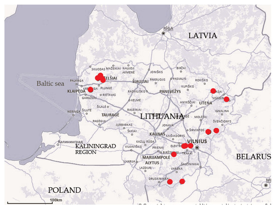
Figure 1.
Map of studied fens (n = 15) in Lithuania (base map: https://www.geoportal.lt/map/ (accessed on 25 July 2025)).

Table 1.
List of investigated fens, their locations, and number of study plots.
Within each study plot, all vascular plant and bryophyte species were recorded, and their abundance was estimated using the Braun–Blanquet cover and abundance scale [55]. The topography was characterised based on microtopography properties (hummock cover, water table position, and surface water presence). Each study plot was assigned to the types of topography following [48], with slight modifications:
- Lawns with negligible microtopography and a high level of surface water that reaches at least half of the bryophyte cover. This usually occurs in flooded areas adjacent to lakes, rivers, or streams.
- Wet lawns (surface water slightly above the peat layer) with shallow hollows.
- Dry lawns (surface water below peat level) with negligible microtopography.
- Hummocky areas (hummocks cover up to 50% of the area).
- Highly hummocky areas (more than 50%) interfacing with deep hollows or water flows.
Additionally, the percentage of hummock cover was evaluated.
Water samples were collected from each plot for hydrochemical analysis. In situ measurements of pH and electrical conductivity were taken using a portable multiparameter device (Multi 350i, WTW, Troistedt, Germany). For chemical analysis, water samples were collected in autumn and frozen until laboratory processing. Concentrations of calcium (Ca2+), magnesium (Mg2+), iron (Fe3+), nitrate (NO3−), ammonium (NH4+), potassium (K+), and phosphate (PO43−) were determined.
Chemical analyses were conducted at the accredited laboratory CJSC “EKOMETRIJA” using standardised ISO and EN ISO methods: Fe3+ (ISO 6332:1995), K+ (ISO 9964-3:1998), NH4+ (ISO 7150-1:1998), NO3− (ISO 7890-3:1998), PO43− (EN ISO 6878:2004), Ca2+ (ISO 6058:2008), and Mg2+ (ISO 6059:2008).
2.3. Data Analysis
Vascular plants and bryophyte groups were distinguished using the TWINSPAN (Two-Way Indicator Species Analysis) algorithm [56], as implemented in the JUICE software. The dataset consisted of species percentage cover values, with pseudo-species cut levels set at 0, 5, 10, and 20%. The classification was terminated at the third cluster level to ensure the resulting groups represented ecologically interpretable floristic units. Species with a fidelity (φ coefficient) exceeding 30% were considered indicator species within each group. The two main TWINSPAN clusters were labelled I–II, with B for bryophytes and H for vascular plants. Groups were numbered 1–11 and similarly marked (e.g., 3B, 5H) for clarity and cross-referencing.
Differences in ecological parameters (hummock cover, pH, topography, conductivity, and concentrations of Ca2+, Mg2+, Fe3+, NO3−, NH4+, K+, and PO43) between plant (IH–IIH) and bryophyte (IB-IIB) clusters identified by the TWINSPAN method were assessed using the Mann–Whitney U test, and differences in the distribution of topography forms were assessed using the Chi-square test. Meanwhile, variations in ecological parameters between vascular plant (1H–11H) and bryophyte (1B–10B) groups were tested using the Kruskal–Wallis test followed by Dunn’s post hoc test. PERMANOVA was used to determine whether the bryophyte and vascular plant groups differed significantly in terms of measured environmental variables. The analysis included species groups identified through classification and a set of measured ecological parameters. Principal component analysis (PCA) was used to identify the main environmental components driving the distribution of vascular plant and bryophyte groups. Components were retained based on the Kaiser criterion, which recommends keeping components with eigenvalues greater than or equal to one [57]. PERMANOVA and PCA were conducted using the PAST statistical software, version 5 [58]. To meet the assumptions of PCA, ecological variables that deviated from a normal distribution (assessed using the Kolmogorov–Smirnov test) were log10-transformed to reduce skewness and approximate normality. The Chi-square test was used to determine the distribution differences between groups of bryophytes and vascular plants. Any p-value less than 0.05 was regarded as statistically significant.
The taxonomic nomenclature followed the checklist of bryophytes of Europe [59] and the World Checklist of Vascular Plants [60].
3. Results
The results of the TWINSPAN in the herb layer illustrated eleven interpreted groups of species (Appendix A). The first cluster (IH), covering groups 1H–5H of the dataset, separated plots with Carex lepidocarpa from the second cluster (IIH), which was mostly characterised by Carex rostrata and Agrostis stolonifera (Appendix A).
Group 1H was characterised by high species richness, in addition to species characteristic to cluster IH (C. lepidocarpa, C. panicea, etc.), including those typical of cluster IIH, such as Agrostis stolonifera, Carex rostrata, and Festuca rubra, which indicates a mixed composition. Similarly, group 6H, assigned to cluster IIH, also exhibited high species diversity and included species from both clusters. However, unlike group 1H, group 6H was much more frequent and abundant in sedges (Carex dioica, C. lepidocarpa, C. nigra, C. panicea, C. rostrata) and shrubs such as Betula pubescens and Salix sp. Group 2H was dominated by low graminoids, especially Eleocharis quinqueflora, while in group 3H, high constancy was demonstrated by Carex panicea. The stands of groups 4H and 5H represented vascular plant compositions with C. lasiocarpa. However, in group 4H, C. lasiocarpa was more strongly associated with other sedges such as C. panicea and C. limosa, whereas group 5H showed a greater presence of Trichophorum alpinum and shrubs (Betula pubescens, Salix sp.).
The second TWINSPAN cluster IIH separated six vegetation groups (6H–11H groups). Group 7H was characterised by the dominance of Eriophorum angustifolium, occurring alongside associated species such as Agrostis stolonifera, Carex diandra, and Caltha palustris. Groups 8H and 9H were both characterised by pronounced hummock formation, suggesting drier fen microtopography. Group 8H included typical mesotrophic fen species such as Carex limosa, Drosera rotundifolia, and Lysimachia thyrsiflora, indicating more open and structurally diverse habitats. By contrast, tall, nutrient-demanding wetland species such as Phragmites australis, Typha latifolia, and Carex diandra occurred exclusively in group 9H. Group 10H included a relatively diverse set of indicators and frequent species such as Agrostis stolonifera, Calla palustris, Caltha palustris, Cardamine pratensis, Eriophorum angustifolium, Festuca rubra, Parnassia palustris, Salix rosmarinifolia, and Silene flos-cuculi. Group 11H, while overlapping in some floristic elements (e.g., Agrostis stolonifera, Caltha palustris) with group 10H, is distinguished by the presence and higher abundance of Carex diandra, C. limosa, Poa trivialis, and Stellaria palustris.
Bryophyte vegetation was classified into two main clusters (IB-IIB) at the first level (TWINSPAN). The IB cluster comprised bryophyte communities with Scorpidium cossonii and Campylium stellatum. The IIB cluster was internally more heterogeneous and primarily associated with species Calliergonella cuspidata and Plagiomnium ellipticum (Appendix B).
The first two bryophyte groups (1B and 2B) represented compositions with Scorpidium cossonii; only group 1B differed from 2B in that it had segments of Sphagnum contortum and Cinclidium stygium, Calliergon giganteum, and Polytrichum strictum, while the bryophyte layer of group 2B was dominated by Scorpidium cossonii. In group 3B, together with Scorpidium cossonii and Campylium stellatum, the bryophyte layer was formed by Plagiomnium elatum and fragments of Tomentypnum nitens, Shagnum teres, Aulacomnium palustre, and Scorpidium scorpioides. The stands of groups 4B and 5B represented different species compositions, with the dominant species Cinclidium stygium and Scorpidium scorpioides in the bryophyte layer. The main difference between these groups lay in their species composition: Group 4B was characterised by the presence of Drepanocladus trifarius, Aulacomnium palustre, Aneura pinguis, and Mesia triquetra and a higher abundance of Campylium stellatum compared to Cinclidium stygium. By contrast, group 5B was notably rich in Cinclidium stygium and Scorpidium scorpioides. Group 6B exhibited high species richness, comprising species characteristic of the first cluster, including Scorpidium cossonii and Campylium stellatum, alongside Aulacomnium palustre and Sphagnum teres, with occasional occurrences of Hamatocaulis vernicosus, Calliergon giganteum, and Climacium dendroides. By contrast, groups 7B and 8B both hosted Hamatocaulis vernicosus, Marchantia polymorpha, and Plagiomnium ellipticum. However, group 8B showed greater species richness, including Brachythecium mildeanum and Tomentypnum nitens, while Calliergon giganteum was found only in group 7B. Groups 9B and 10B were distinguished by Sphagnum sp., Paludella squarrosa, and Tomentypnum nitens, while group 10B was notable for the abundance of Helodium blandowii.
The Mann–Whitney U test revealed significant differences in environmental variables between the two vascular plant clusters (Table 2). Specifically, pH and the concentrations of Mg2+, Fe3+, NH4+, PO43−, and K+ differed significantly, with most of these elements being more abundant in cluster IIH. Similarly, when comparing the corresponding bryophyte clusters, significant differences were observed in hummock cover, pH (with cluster IB being more alkaline), and the concentrations of Fe3+, K+, Mg2+, and PO43−. As in the vascular plant dataset, these variables were generally more abundant and exhibited broader ranges within cluster IIB of the bryophyte groups.
Table 2.
Statistical comparisons of environmental parameters (hummock cover; pH; conductivity; concentrations of Ca2+, Fe3+, K+, Mg2+, NH4+, NO3−, and PO43−; and topography type) between vascular plant (I-IIH) and bryophyte (I-IIB) clusters. All environmental parameters were analysed using the Mann–Whitney U test, while differences in the distribution of topography forms were assessed using the Chi-square test. Significant differences (p < 0.05) are highlighted in bold.
The PCAs were conducted exclusively between vascular plant groups and bryophyte groups to identify the key environmental variables influencing species composition (Table 3). Among the ten measured environmental factors, hummock cover, topography, and iron concentration consistently emerged as the most influential in explaining the variation within both vascular and bryophyte groups (Figure 2). Although the same environmental factors were significant across all groups, their relative contributions differed, i.e., hummock cover had the most decisive influence on bryophyte communities, while topography more strongly affected vascular plant species distribution.
Table 3.
PCA loadings of environmental parameters (hummock cover, topography type, pH, conductivity, and concentrations of Ca2+, Fe3+, K+, Mg2+, NH4+, NO3−, and PO43−) and species groups (vascular plants and bryophytes) across study sites (n = 98). Loadings in bold indicate high contributions (|loading| > 0.4).
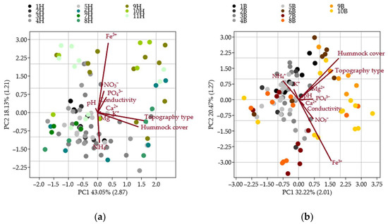
Figure 2.
Principal component analysis (PCA) of environmental variables (hummock cover, topography type, pH, conductivity, and concentrations of Ca2+, Fe3+, K+, Mg2+, NH4+, NO3−, and PO43−) influencing the distribution of vascular plant (1H–11H) (a) and bryophyte (1B–10B) (b) groups; each colour represents a different group based on components (PC) with eigenvalues greater than one (eigenvalues shown in parentheses on axes).
Environmental parameters associated with the five bryophyte groups (1B–5B) and five vascular plant groups (1H–5H) generally reflect stable, moderately calcium-rich conditions with limited variation in key ecological factors. However, among vascular plant groups, group 1H stood out due to lower conductivity and elevated concentrations of magnesium and potassium. By contrast, bryophyte groups (1B–5B) showed more apparent ecological differentiation, particularly in terms of pH and hummock cover, with group 2B exhibiting notably higher levels of magnesium and potassium (Figure 3 and Figure 4).
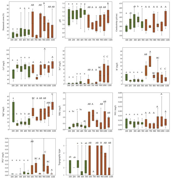
Figure 3.
Comparison of ecological variables (hummock cover; pH; conductivity; concentrations of Ca2+, Fe3+, K+, Mg2+, NH4+, NO3−, and PO43−; and topography types) among vascular plant groups (1H–11H) using boxplots, showing significant differences in environmental conditions. Colours represent different clusters assigned to each group. Lowercase letters indicate statistically significant differences among groups within cluster IH, while uppercase letters indicate differences among groups within cluster IIH. Statistical differences were tested using the Kruskal–Wallis test followed by Dunn’s post hoc test (p < 0.05).
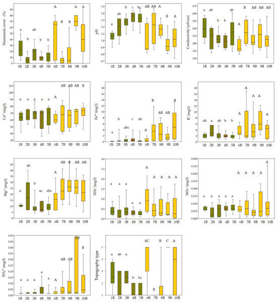
Figure 4.
Comparison of ecological variables (hummock cover; pH; conductivity; concentrations of Ca2+, Fe3+, K+, Mg2+, NH4+, NO3−, and PO43−; and topography type) among bryophyte groups (1B–10B) using boxplots, showing significant differences in environmental conditions. Colours represent different clusters assigned to each group. Lowercase letters indicate statistically significant differences among groups within cluster IB, while uppercase letters indicate differences among groups within cluster IIB. Statistical differences were tested using the Kruskal–Wallis test followed by Dunn’s post hoc test (p < 0.05).
In the case of the vascular plant groups from the second cluster IIH, the species-rich group 6H, characterised by greater hummock cover, preferred a slightly higher availability of NO3−, NH4+, Mg2+, and K+. Patches with Eleocharis quinqueflora (group 7H) thrived in mineral-rich, wet, and slightly more acidic conditions, exhibiting lower Ca2+, Fe3+, and NO3− but the highest concentrations of K+ compared to other IIH groups. Groups 8H and 9H were associated with the development of hummocks and mineral-rich conditions. On the other hand, group 9H was more relevant to higher Fe3+ and PO43− concentrations. Group 10H shared similar environmental conditions with group 11H, both being associated with rich and moist habitat features. However, group 11H was distinguished by slightly wetter conditions, higher electrical conductivity, and lower pH values as well as lower PO43− (Figure 3).
Vegetation patterns across the identified Calliergonella cuspidata and Plagiomnium ellipticum groups (6B–10B) were strongly influenced by microtopography and water chemistry. Group 6B was characterised by drier microsites and low Fe3+ and conductivity, but high NO3− and NH4+. By contrast, groups 7B and 8B represented wetter, base-rich areas with higher Fe3+, Mg2+, and conductivity and were ecologically similar. Groups 9B and 10B were marked by hummock development and high concentrations of Mg2+, Fe3+, and PO43−, with group 9B exhibiting especially elevated K+ and PO43− (Figure 4).
PERMANOVA results revealed significant differences among bryophyte groups based on the measured environmental variables, indicating that bryophyte communities exhibited greater ecological differentiation compared to vascular plant groups (Table 4 and Table 5).
Table 4.
Pairwise vascular plant group differences based on PERMANOVA of environmental parameters (hummock cover, topography type, pH, conductivity, and concentrations of Ca2+, Fe3+, K+, Mg2+, NH4+, NO3−, and PO43−). Significant differences (p < 0.05) are highlighted in bold.
Table 5.
Pairwise bryophyte group differences based on PERMANOVA of environmental parameters (hummock cover, topography type, pH, conductivity, and concentrations of Ca2+, Fe3+, K+, Mg2+, NH4+, NO3−, and PO43−). Significant differences (p < 0.05) are highlighted in bold.
The joint distribution of bryophyte and vascular plant groups highlights apparent asymmetries in the ecological amplitude and habitat specificity of vascular plant groups of different clusters. Bryophyte groups 1B–5B were closely related to vascular plant groups of the IH cluster, while 7B–10B bryophyte groups were with the vascular groups from the IIH cluster (Figure 5).
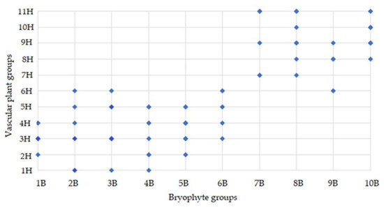
Figure 5.
Binary association matrix illustrating ecological group-level relationship between vascular plant (1H–11H) (Appendix A) and bryophyte groups (1B–10B) (Appendix B) (based on co-occurrence in study sites).
4. Discussion
4.1. Main Characteristics of Bryophyte and Vascular Plant Covers in the Studied Fens
As in the northeastern part of Poland [49] neighbouring Lithuania, the communities we studied, based on vascular plant cover, are divided into two clusters based on the distribution of Carex lepidocarpa and C. rostrata. Concerning the C. lepidocarpa cluster, most of the diagnostic species (C. panicea, Drosera anglica, Eleocharis quinqueflora, Eriophorum latifolium, Peucedanum palustre) are the same [49]. Additionally, the communities we described are also characterised by the presence of Trichophorum alpinum, which is found in various parts of Europe, growing together with previously mentioned species [61]. The species Epipactis palustris and Cirsium palustre, indicated as diagnostic for the Carex lepidocarpa cluster [49], were found equally distributed in both clusters. In the newest synthesis of fen alliances of Europe, only C. panicea and Eriophorum latifolium are indicated as diagnostic for Caricion davallianae communities. The other species mentioned have no diagnostic role in any of the alliances.
In addition to the species Agrostis stolonifera, Carex diandra, Epilobium palustre, Ranunculus lingua, Rumex acetosa, and Silene flos-cuculi, which are provided as characteristic of Poland fen communities indicated by Carex rostrata [49], we found that this cluster is also marked by Caltha palustris, Festuca rubra, Galium uliginosum, and Myosotis scorpioides. Usually, Carex rostrata stands belong to Caricetum rostratae (Caricion rostratae, Magnocaricetalia) [62]. The water level is an essential factor for the growth of C. rostrata shoots, especially during early summer when most of the length increment occurs [63]. Carex rostrata and plants with high stem porosity are adaptive to growing in areas with high Fe3+ concentrations [64]. Carex rostrata usually has high fidelity in the habitats of alliances Stygio-Caricion limosae, Sphagno-warnstorfii Tomentypnion, Saxifrago-Tomentypnion, and Sphagno caricion canescentis [40].
Unlike previous research [49], which was focused exclusively on bryophyte carpets, our study incorporated plots displaying a variety of microtopographic features. This allowed us to reveal a greater diversity of bryophytes in both clusters, including Cinclidium stygium, Drepanocladus trifarius, Meesia triquetra, Paludella squarrosa, Helodium blandowii, and Sphagnum species. Despite the greater diversity of bryophytes, the two main clusters featured similar species to those in the Polish study [49].
Similar to the vascular plant communities from the IH cluster, bryophytes of the IB cluster, indicated by Campylium stellatum and Scorpidium cossonii, also prefer rich fens characterised by stable or only slightly fluctuating water tables and higher pH values, which is consistent with the Polish findings [49].
In the compendium of fen alliances [40], it is indicated that C. stellatum reaches the highest frequency in Caricion davallianae, Caricion atrofusco saxatilis, and Sphagno warnstorfii-Tomentypnion alliances; however, the diagnostic role of Scorpidium cossonii in this compendium is not defined, as the species is integrated into an ecologically wider, especially according to habitat acidity [65], assemblage aggr. Drepanocladus revolvens.
Hamatocaulis vernicosus, Marchantia polymorpha, and Plagiomnium ellipticum, the diagnostic species of the IIB cluster, also distinguish one of the vegetation groups in the Polish study [49]. It is important to emphasise that our research revealed Calliergonella cuspidata and Plagiomnium ellipticum to play a more significant role in distinguishing the two clusters than the other species mentioned. C. cuspidata and P. ellipticum usually thrive within the same general habitat but occupy different micro-niches. Calliergonella cuspidata is typically found in more open habitats with higher nutrient content, such as base-rich fens. It prefers moderately moist-to-wet substrates with stable hydrological conditions but can tolerate a range of moisture regimes [61,66,67]. In some studies [16,19,68], C. cuspidata is commonly recognised as an indicator species of both eutrophication and drying conditions in fen ecosystems. Plagiomnium ellipticum prefers shaded areas with stable hydrological conditions. It is often found in slightly wetter areas, forming dense patches in depressions or shallow hollows where water accumulates [65,69]. These species co-occur not because they are ecologically similar, but because they have overlapping tolerance ranges that enable them to thrive under specific environmental conditions.
Our results are consistent with the findings by Pawlikowski et al. [49], showing a strong co-occurrence between Plagiomnium ellipticum and Hamatocaulis vernicosus and suggesting that these species may share similar ecological preferences. Meanwhile, Calliergonella cuspidata has been found by Pawlikowski [49] to occur with similar frequency across two floristically distinct rich fen types. By contrast, our study, as well as previous studies [48,61,70,71], suggest that C. cuspidata is less prevalent in fens dominated by Scorpidium cossonii in the bryophyte layer. This may be attributed to the differing ecological requirements of the two species. Calliergonella cuspidata prefers more nutrient-rich habitats and is better adapted to dynamic fen environments than Scorpidium cossonii [19,68].
Although we analysed bryophyte and plant diversity separately, our study confirms the two groups of fen vegetation found in Poland [49] and provides further evidence of their ecological differences at a broader geographic scale. Additionally, in line with the pH differences between the plant clusters ascertained by Pawlikowski et al. [49], we observed significant differences in pH and the amounts of Ca2+, Fe3+, Mg2+, K+, NO3−, and PO43− in their habitats. This may be associated with the regional characteristics of the fens, which, in most cases, are fed by mineral-rich springs (especially iron-rich ones) [72]. Usually, Carex lepidocarpa is provided as an indicator of calcareous fens. However, calcium levels were higher in Carex rostrata than in C. lepidocarpa communities in the fens we studied. This confirms the need to obtain reliable data from a wider area of Eastern Europe to specify the composition, ecology, and distribution pattern of the plant communities formed by C. rostrata and C. diandra [49].
4.2. Mosaic Structure of Vascular Plant Cover
The two main clusters of vascular plants and bryophytes reflect the regional peculiarities of Lithuanian fens. The further distinguished groups of species pools reflect the mosaic structure of fen communities, which may be defined by local ecological conditions.
The distributions of vascular plant groups are in accordance with the insight that water level is one of the important axial factors influencing the distribution of vascular plants in fen communities, and it is the major determinant of small-scale patterns of species distribution [37]. Water level, in our study, is indirectly presented as topography, and is a key factor in determining the mosaic nature of the plant communities in the C. lepidocarpa cluster, where most of the chemical parameters are similar. The indicator species for the vegetation pools in this cluster are usually Eleocharis quinqueflora, Carex panicea, and C. lasiocarpa. The patches dominated by Eleocharis quinqueflora occur at water-saturated sites of calcareous fens [73]. Carex panicea is a characteristic species of fen meadows. The investigations of drained fens in Sweden show the C. panicea peak at five to ten years after drainage [23]. Thus, the extension of such communities in the fens may be an indication of their encroachment. According to [74], plant communities with C. lasiocarpa and calciphilous species represent the wetter face of Caricion davallianae. The wetter characteristic in our study is also indicated by the species growing together: Carex diandra, C. limosa, Comarum palustre, etc.
Vegetation heterogeneity may be enhanced by an expanding shrub and tree cover, which is often linked to a drop in water levels and hummocky character of the area [23]. The occurrence of shrubs (Salix rosmarinifolia), meadow species (Rumex acetosa, Silene flos-cuculi, and Festuca rubra), and wetland plants (e.g., Carex limosa, Calle palustris, Caltha palustris) in the same vegetation pool reflects the co-occurrence of hummocks and the hollows.
When analysing the differences between the two clusters as well as within IIH, we found that iron content is also a key factor in determining the mosaic structure of their vegetation. The content of this toxic metallic element can influence patterns of small-scale vegetation [37,38]. Extremely high iron was fixed within the vegetation patches of the 9H, 10H, and 11H groups. However, many species characteristic of these groups, such as Agrostis stolonifera, Caltha palustris, and Calle palustris, are also common in habitats with lower iron content (group 7H). For plants inhabiting fens fed by iron-rich waters, high iron concentrations are probably not necessary but are tolerable. We found that, in addition to these species, the patches with low iron and calcium were dominated by Eriophorum angustifolium. Usually, E. angustifolium communities are basic elements of mire vegetation in Sphagnum peatlands [75]. However, the species can tolerate a wide range of pH values (3.7–6.8), nitrates, base deficiency, and iron [76]. The high amount of potassium recorded by us in the patches dominated by E. angustifolium seems to be limited by potassium as in the case of E. vaginatum [77]. Another distinguishing feature of this group habitat is the high levels of ammonium coupled with low amounts of nitrates. This may be related to the high water levels in the habitat, which could be affecting the reduction processes [18]. Two groups indicated by Carex limosa (8H and 11H) are distinguished by a greater extent of surface water or the presence of hollows, as well as by a low amount of phosphorus content. The species exhibits characteristics (a low fresh shoot ratio) that may help it grow under low phosphate conditions [78].
It is important to note that two groups (1H and 6H) are classified in different clusters, although they share diagnostic species that are specific to both. Group 6H, attributed to the C. rostrata cluster, is defined by the presence of C. dioica and C. nigra. The latter is a diagnostic species of the Caricion fuscae alliance and occurs in habitats with moderate-to-low calcium content [40]. Although our studies do not indicate any differences in calcium content between these groups, group 6H is closer to cluster IIH in terms of other parameters.
4.3. Bryophyte Pools and Their Ecological Preferences
As with vascular plant groups, the heterogeneity of rich fens, as manifested through features such as water levels, hummocks, and hollows, shapes the distribution patterns of bryophyte groups observed in our study. Patches indicated by Scorpidium scorpioides and Cinclidium stygium, along with inclusions of Drepanocladus trifarius, Meesia triquetra, and Aneura pinguis, as well as bryophyte groups dominated by species such as Hamatocaulis vernicosus and Calliergon giganteum, were more strongly tied to stable, waterlogged hollows or lawns, where water availability remains consistently high. This finding is consistent with previous experiments, which have shown that these species exhibit high vitality under prolonged waterlogged conditions [18]. By contrast, patches dominated by Scorpidium cossonii and Campylium stellatum appear to indicate that the water table lay somewhat deeper.
Groups 6B, 9B, and 10B represent bryophyte species that actively form hummocks. Likewise, Paludella squarrosa and Helodium blandowii, typically considered indicators of wetter environments [65], were frequently associated with low hummocks in relatively dry microsites in our study, suggesting a broader ecological amplitude and potential adaptation to spatial moisture variability [67]. Hummock formation by bryophytes, especially those with high water-holding capacity and dense canopy structure, not only reduces desiccation stress but also contributes to fen stability or, conversely, promotes ecological shifts by altering hydrological feedback [79,80,81]. Moreover, our findings support previous studies e.g., [82,83,84], indicating that increased hummock abundance is often linked to declining pH values. Wet carpets dominated by species like Hamatocaulis vernicosus and Scorpidium scorpioides occur under slightly alkaline conditions, while areas with more hummock-forming species are associated with more acidic habitats.
It is also crucial to highlight the role of iron content in shaping the spatial patterns of bryophytes. In fen habitats, iron plays a crucial role in phosphorus cycling, which in turn affects plant growth and overall ecosystem health [64]. Patches dominated by Hamatocaulis vernicosus were commonly found in areas with high iron concentrations, although this species showed tolerance to a wide range of iron levels [48]. Although the presence of H. vernicosus is associated with higher phosphorus levels [49], our previous research [48] and the current study do not show that these species habitats are distinguished by their phosphorus content. Additionally, high iron levels were also recorded in hummocky group 10B. At the same time, phosphorus exhibited a notably wide range of values in group 9H—with frequent patches of Palludella squarrosa in the bryophyte layer. This variability in phosphorus and iron concentrations warrants further detailed analysis, as it may reflect localised environmental heterogeneity. Potential factors include differences in redox conditions, organic matter decomposition, and microtopography (e.g., presence of hollows and hummocks) [18,85].
Our study found high levels of base cations (Ca2+, Mg2+, and K+) in rich fens, although these factors appeared to have only a moderate influence on the distribution of bryophyte groups. Unlike some reports linking Scorpidium cossonii to higher calcium levels [72,86,87], we observed no significant calcium differences, but the ratio of calcium to magnesium and potassium appeared more relevant [84]. Additionally, hummocky areas with patches of Paludella squarrosa and Helodium blandowii exhibited notably higher potassium levels, ranging from five to six mg/L. In terms of NH4+ concentrations, they were notably higher and more variable, with several sites exceeding two mg/L, indicating potential organic pollution [88] or reduced oxygen conditions in groups 6B and 10B. These findings suggest that the bryophyte communities observed in these groups may be subjected to elevated environmental stress or anthropogenic disturbance [50].
4.4. Vascular and Bryophyte Groups as Indicators of Habitat Conditions
Our study indicates that the distribution of bryophyte and vascular plant groups is primarily influenced by the same factors: topography, number of hummocks, and iron content. However, vascular plant groups exhibit a wider range of overlaps with ecological conditions compared to bryophyte groups. Vegetation patches defined by the same vascular plant assemblages or dominant plant species may cover bryophyte pools with a different species composition. Vascular plants are less sensitive to microtopographic or hydrological changes than are bryophytes due to their more efficient water conducting system. They can penetrate deeper into peat layers and are thus expected to sustain water uptake and, consequently, transpiration [89,90]. In addition, the development of vascular plants, such as sedges, may be determined by competition between species due to their different life traits. The gaps in the vegetation that are necessary for seed germination and seedling establishment are often unavailable in dense stands of rhizomatous, clonal species [91]. Therefore, initial changes in environmental conditions in fens may be more accurately identified by changes in the composition of bryophytes than by vascular plants. As Hajek et al. [19] stated, shifts in bryophyte species composition also indicate undesirable successional changes in fens. Conversely, the diversity of bryophytes may be linked to slight differences in micro-relief that persist despite general changes in the fen’s hydrology. It is essential to note that, when evaluating changes in habitat conditions, identifying the exact species, not just complexes of species, is crucial.
Nonetheless, there is significant overlap between specific plant and bryophyte groups within the clusters, while the differences between the clusters are pronounced. The exclusion of intermediate groups between the respective clusters of vascular plants (6H) and bryophytes (6B) makes this particularly striking. On one side, there are the fen communities characterised by Carex lepidocarpa and Scorpidium cossonii and, on the other, those characterised by Carex rostrata and Hamatocaulis vernicous. This shows once again that such fens are common in the region, which is transitional between the boreal and continental regions. There are two distinct types of fens, which are significantly different in their species composition from those described in Central Europe [48,49]. We agree with Pawlikowski et al. [49] that the fens we described do not exactly fit the scheme according to the poor-rich gradient provided for Central Europe [68]. Most importantly, it has no place for the plant communities characterised by the most typical species, including Carex rostrata, C. diandra, Agrostis stolonifera, Caltha palustris, and Hamatocaulis vernicosus in the moss cover. While such fen habitats are abundant in calcium and minerals, they do not contain calcareous species, as has also been reported by Pawlikowski [49]. Although H. vernicosus is listed as a characteristic of extremely rich fen species in the scheme [68], these fens are also characterised by the presence of Scorpidium cossonii and Campylium stellatum. The only bryophyte group that harbours both Hamatocaulis vernicosus and Scordidium cossonnii and meets the group’s criteria for calcareous vascular plants is group 6B. Therefore, there is still scope for debate on how the fens in our region should be divided.
5. Conclusions
Our research identified two ecologically and floristically distinct plant communities that are representative of regional fen ecosystems. Such data are highly relevant for the fen classification efforts at both the national and European scales. The mosaic distribution of vegetation, observed in both bryophyte and vascular plant layers, is primarily shaped by local hydrological regimes, microtopographical variation, and the amount of iron. Given their greater ecological differentiation, bryophyte assemblages serve as particularly sensitive indicators and should be given special attention in conservation planning and habitat management.
Author Contributions
Conceptualization, I.J.; methodology, I.J. and M.K.; data curation, M.K.; formal analysis, I.J. and M.K.; investigation, M.K. and. I.J.; writing—original draft preparation, M.K. and I.J.; visualisation, M.K.; supervision, I.J.; writing—review and editing, I.J. and M.K. All authors have read and agreed to the published version of the manuscript.
Funding
This research received no external funding.
Data Availability Statement
The data presented in this study are available upon request from the corresponding author. The data are not publicly available due to privacy concerns.
Acknowledgments
We are grateful to Zofija Sinkevičienė for providing valuable information. We want to thank Dalytė Matulevičiūtė and Lukas Petrulaitis for help in the identification of vascular plant species, as well as Viktoras Subka and Gabrielė Jociūtė for their kind assistance during fieldwork.
Conflicts of Interest
The authors declare no conflicts of interest.
Appendix A
Table A1.
Results of TWINSPAN classification showing species presence, frequency, and φ coefficients for indicator species across different vascular plant groups (1H–11H). Columns represent vascular plant groups, rows represent species, and each cell contains species frequency with the φ coefficient indicated as a superscript. Dominant species were those with a frequency greater than 50% and a φ coefficient above 30 (φ coefficient expressed as a percentage, i.e., multiplied by 100).
Appendix B
Table A2.
Results of TWINSPAN classification showing species presence, frequency, and φ coefficients for indicator species across different bryophyte groups (1B–10B). Columns represent bryophyte groups, rows represent species, and each cell contains species frequency with the φ coefficient indicated as a superscript. Dominant species were those with a frequency greater than 50% and a φ coefficient above 30 (φ coefficient expressed as a percentage, i.e., multiplied by 100), indicating frequent occurrence and strong association with the respective group.
References
- European Environment Agency. European Biodiversity Strategy for 2030. Available online: https://ec.europa.eu/environment/nature/biodiversity/strategy/index_en.htm (accessed on 30 June 2025).
- Wu, Y.; Tao, Y.; Yang, G.; Ou, W.; Pueppke, S.; Sun, X.; Chen, G.; Tao, Q. Impact of land use change on multiple ecosystem services in the rapidly urbanizing Kunshan City of China: Past trajectories and future projection. Land Use Policy 2019, 85, 419–427. [Google Scholar] [CrossRef]
- Hicks, L.L.; Vogel, W.O.; Herter, D.R.; Early, R.J.; Stabins, H.C. Plum creek’s central cascades habitat conservation plan and modeling for the northern spotted owl. In Models for Planning Wildlife Conservation in Large Landscapes; Millspaugh, J.J., Thomsin, F.R., Eds.; Academic Press: Cambridge, MA, USA, 2009; pp. 561–592. [Google Scholar] [CrossRef]
- Jukonienė, I.; Kalvaitienė, M.; Bagušinskaitė, A. Bryophyte diversity as an indication of habitat quality in two special areas of conservation on the outskirts of Vilnius (Verkiai Regional Park). Botanica 2022, 28, 159–170. [Google Scholar] [CrossRef]
- Ghasemi, M.; González-García, A.; Serrao-Neumann, S. Ecosystem services modelling to analyse the isolation of protected areas from a social-ecological perspective. J. Environ. Manag. 2025, 386, 125459. [Google Scholar] [CrossRef]
- Beninde, J.; Veith, M.; Hochkirch, A. Biodiversity in cities needs space: A meta-analysis of factors determining intra-urban biodiversity variation. Ecol. Lett. 2015, 18, 581–592. [Google Scholar] [CrossRef] [PubMed]
- Lamers, L.P.M.; Vile, M.A.; Grootjans, A.P.; Acreman, M.C.; van Diggelen, R.; Evans, M.G.; Richardson, C.J.; Rochefort, L.; Kooijman, A.M.; Roelofs, J.G.M.; et al. Ecological restoration of rich fens in Europe and North America: From trial and error to an evidence-based approach. Biol. Rev. 2015, 90, 182–203. [Google Scholar] [CrossRef] [PubMed]
- Bedford, B.L.; Godwin, K.S. Fens of the United States: Distribution, characteristics, and scientific connection versus legal isolation. Wetlands 2003, 23, 608–629. [Google Scholar] [CrossRef]
- Schot, P.P.; Wassen, M.J. Calcium concentrations in wetland groundwater in relation to water sources and soil conditions in the recharge area. J. Hydrol. 1993, 141, 197–217. [Google Scholar] [CrossRef]
- Hájek, M.; Jiménez-Alfaro, B.; Hájek, O.; Brancaleoni, L.; Cantonati, M.; Carbognani, M.; Dedić, A.; Ditĕ, D.; Gerdol, R.; Hájková, P.; et al. European map of groundwater pH and calcium. Earth Syst. Sci. Data Discuss. 2021, 13, 1089–1105. [Google Scholar] [CrossRef]
- van Haesebroeck, V.; Boeye, D.; Verhagen, B.; Verheyen, R.F. Experimental investigation of drought induced acidification in a rich fen soil. Biogeochemistry 1997, 37, 15–32. [Google Scholar] [CrossRef]
- Beltman, B.; Van den Broek, T.; Barendregt, A.; Bootsma, M.C.; Grootjans, A.P. Rehabilitation of acidified and eutrophied fens in The Netherlands: Effects of hydrologic manipulation and liming. Ecol. Eng. 2001, 17, 21–31. [Google Scholar] [CrossRef]
- Kooijman, A.; Paulissen, M.P.C.P. Higher acidification rates in fens with phosphorus enrichment. Appl. Veg. Sci. 2006, 9, 205–212. [Google Scholar] [CrossRef]
- van Diggelen, J.M.; Bense, I.H.; Brouwer, E.; Limpens, J.; van Schie, J.M.; Smolders, A.J.; Lamers, L.P. Restoration of acidified and eutrophied rich fens: Long-term effects of traditional management and experimental liming. Ecol. Eng. 2015, 75, 208–216. [Google Scholar] [CrossRef]
- Karpińska-Kołaczek, M.; Kołaczek, P.; Czerwiński, S.; Gałka, M.; Guzowski, P.; Lamentowicz, M. Anthropocene history of rich fen acidification in W Poland—Causes and indicators of change. Sci. Total Environ. 2022, 838, 155785. [Google Scholar] [CrossRef]
- Kooijman, A.M. Poor rich fen mosses’: Atmospheric N-deposition and P-eutrophication in base-rich fens. Lindbergia 2012, 35, 42–52. [Google Scholar]
- Wassen, M.; Venterink, H.; Lapshina, E.; Tanneberger, F. Endangered plants persist under phosphorus limitation. Nature 2005, 437, 547–550. [Google Scholar] [CrossRef]
- Cusell, C.; Lamers, L.P.; van Wirdum, G.; Kooijman, A. Impacts of water level fluctuation on mesotrophic rich fens: Acidification vs. eutrophication. J. Appl. Ecol. 2013, 50, 998–1009. [Google Scholar] [CrossRef]
- Hájek, M.; Jiroušek, M.; Navrátilová, J.; Horodyská, E.; Peterka, T.; Plesková, Z.; Navrátil, J.; Hájková, P.; Hájek, T. Changes in the moss layer in Czech fens indicate early succession triggered by nutrient enrichment. Preslia 2015, 87, 279–301. [Google Scholar]
- Janssen, J.A.; Rodwell, J.S.; Criado, M.G.; Gubbay, S.; Haynes, T.; Nieto, A.; Sanders, N.; Landucci, F.; Loidi, J.; Ssymank, A.; et al. European Red List of Habitats Part 2. Terrestrial and Freshwater Habitats; European Union: Brussels, Belgium, 2016. [Google Scholar]
- Rion, V.; Gallandat, J.D.; Gobat, J.M.; Vittoz, P. Recent changes in the plant composition of wetlands in the Jura Mountains. Appl. Veg. Sci. 2018, 21, 121–131. [Google Scholar] [CrossRef]
- Geurts, J.J.; Sarneel, J.M.; Willers, B.J.; Roelofs, J.G.; Verhoeven, J.T.; Lamers, L.P. Interacting effects of sulphate pollution, sulphide toxicity and eutrophication on vegetation development in fens: A mesocosm experiment. Environ. Pollut. 2009, 157, 2072–2081. [Google Scholar] [CrossRef] [PubMed]
- Mälson, K.; Backéus, I.; Rydin, H. Long-term effects of drainage and initial effects of hydrological restoration on rich fen vegetation. Appl. Veg. Sci. 2008, 11, 99–106. [Google Scholar] [CrossRef]
- Booth, E.G.; Loheide, S.B.; Bart, D. Fen ecohydrological trajectories in response to groundwater drawdown with edaphic feedback. Ecohydrology 2022, 15, e2471. [Google Scholar] [CrossRef]
- Shih, J.G.; Finkelstein, S.A. Range dynamics and invasive tendencies in Typha latifolia and Typha angustifolia in eastern North America derived from herbarium and pollen records. Wetlands 2008, 28, 1–16. [Google Scholar] [CrossRef]
- Pyšek, P.; Chytrý, M.; Pergl, J.; Sádlo, J.; Wild, J. Plant invasions in the Czech Republic: Current state, introduction dynamics, invasive species and invaded habitats. Preslia 2012, 84, 575–629. [Google Scholar]
- Dube, C.; Pellerin, S.; Poulin, M. Do power line rights-of-way facilitate the spread of non-peatland and invasive plants in bogs and fens? Botany 2011, 89, 91–103. [Google Scholar] [CrossRef]
- Essl, F.; Dullinger, S.; Moser, D.; Rabitsch, W.; Kleinbauer, I. Vulnerability of mires under climate change: Implications for nature conservation and climate change adaptation. Biodivers. Conserv. 2012, 21, 655–669. [Google Scholar] [CrossRef]
- Kolari, T.H.M.; Korpelainen, P.; Kumpula, T.; Tahvanainen, T. Accelerated vegetation succession but no hydrological change in a boreal fen during 20 years of recent climate change. Ecol. Evol. 2021, 11, 7602–7621. [Google Scholar] [CrossRef] [PubMed]
- Moen, A.; Lyngstad, A.; Øien, D.I. Hay crop of boreal rich fen communitiest raditionally used for haymaking. Folia Geobot. 2015, 50, 25–38. [Google Scholar] [CrossRef]
- Hájková, P.; Horsáková, V.; Peterka, T.; Janeček, Š.; Galvánek, D.; Dítě, D.; Horník, J.; Horsák, M.; Hájek, M. Conservation and restoration of Central European fens by mowing: A consensus from 20 years of experimental work. Sci. Total Environ. 2022, 846, 157293. [Google Scholar] [CrossRef]
- Wheeler, B.D.; Shaw, S.C.; Fojt, W.J.; Robertson, R.A. (Eds.) Restoration of Temperate Wetlands, 1st ed.; Wiley: Hoboken, NJ, USA, 1995; 562p. [Google Scholar]
- EUNIS. Habitat Classification. Available online: https://www.eea.europa.eu/data-and-maps/data/eunis-habitat-classification-1/eunis-terrestrial-habitat-classification-review-2021 (accessed on 21 May 2025).
- European Commission. Council Directive 92/43/EEC of 21 May 1992 on the conservation of natural habitats and of wild fauna and flora. Off. J. Eur. Union 1992, 206, 7–50. [Google Scholar]
- Jiménez-Alfaro, B.; Fernández-Pascual, E.; Díaz González, T.E.; Peréz-Haase, A.; Ninot, J.M. Diversity of rich fen vegetation and related plant specialists in mountain refugia of the Iberian Peninsula. Folia Geobot. 2012, 47, 403–419. [Google Scholar] [CrossRef]
- Jiménez-Alfaro, B.; Hájek, M.; Ejrnaes, R.; Rodwell, J.; Pawlikowski, P.; Weeda, E.J.; Laitinen, J.; Moen, A.; Bergamini, A.; Aunina, L.; et al. Biogeographic patterns of base-rich fen vegetation across Europe. Appl. Veg. Sci. 2014, 17, 367–380. [Google Scholar] [CrossRef]
- Hájková, P.; Hájek, M. Bryophyte and vascular plant responses to base-richness and water level gradients in Western Carpathian Sphagnum-rich mires. Folia Geobot. 2004, 39, 335–351. [Google Scholar] [CrossRef]
- Hájková, P.; Hájek, M. Species richness and above-ground biomass of poor and calcareous spring fens in the flysch West Carpathians, and their relationships to water and soil chemistry. Preslia 2003, 5, 271–287. [Google Scholar]
- Hájek, M.; Dítě, D.; Horsáková, V.; Mikulášková, E.; Peterka, T.; Navrátilová, J.; Jiménez-Alfaro, B.; Hájková, P.; Tichy, L.; Horsák, M. Towards the pan-European bioindication system: Assessing and testing updated hydrological indicator values for vascular plants and bryophytes in mires. Ecol. Indic. 2020, 116, 106527. [Google Scholar] [CrossRef]
- Peterka, T.; Hájek, M.; Jiroušek, M.; Jiménez-Alfaro, B.; Aunina, L.; Bergamini, A.; Dítě, D.; Felbaba-Klushyna, L.; Graf, U.; Hájková, P.; et al. Formalized classification of European fen vegetation at the alliance level. Appl. Veg. Sci. 2017, 20, 124–142. [Google Scholar] [CrossRef]
- Øien, D.-I. Nutrient limitation in boreal rich-fen vegetation: A fertilization experiment. Appl. Veg. Sci. 2004, 7, 119–132. [Google Scholar] [CrossRef]
- Vitt, D.H.; Hopuse, M.; Glaeser, L. The response of vegetation to chemical and hydrological gradients at a patterned rich fen in northern Alberta, Canada. J. Hydrol. Reg. Stud. 2022, 40, 101038. [Google Scholar] [CrossRef]
- van Der Hoek, D.; van Mierlo, A.J.E.M.; van Groenendael, J.M. Nutrient limitation and nutrient-driven shifts in plant species composition in a species-rich fen meadow. J. Veg. Sci. 2004, 15, 389–396. [Google Scholar] [CrossRef]
- Kay, S.; Proctor, J. Population dynamics of two Scottish ultramafic (serpentine) rarities with contrasting life histories. Bot. J. Scotl. 2003, 55, 269–285. [Google Scholar] [CrossRef]
- van der Maarel, E. On the establishment of plant community boundaries. Berichte Dtsch. Bot. Ges. 1976, 89, 415–443. [Google Scholar] [CrossRef]
- van der Maarel, E. Ecotones and ecoclines are different. J. Veg. Sci. 1990, 1, 135–138. [Google Scholar] [CrossRef]
- Eppinga, M.B.; Michaels, T.K.; Santos, M.J.; Bever, J.D. Introducing desirable patches to initiate ecosystem transitions and accelerate ecosystem restoration. Ecol. Appl. 2023, 33, e2910. [Google Scholar] [CrossRef]
- Kalvaitienė, M.; Jukonienė, I. Habitat preferences of Hamatocaulis vernicosus at the junction of continental and boreal phytogeographical regions (Lithuania). Boreal Environ. Res. 2022, 27, 81–96. [Google Scholar]
- Pawlikowski, P.; Abramczyk, K.; Szczepaniuk, A.; Kozub, Ł. Nitrogen: Phosphorus ratio as the main ecological determinant of the differences in the species composition of brown-moss rich fens in north-eastern Poland. Preslia 2013, 85, 349–367. [Google Scholar]
- Jabłońska, E.; Pawlikowski, P.; Jarzombkowski, F.; Tarapata, M.; Kłosowski, S. Thirty years of vegetation dynamics in the Rospuda fen (NE Poland). Mires Peat 2019, 24, 05. [Google Scholar] [CrossRef]
- Auniņa, L. Vegetation changes in extremely rich fens in Latvia. Rend. Fis. Acc. Lincei 2022, 33, 707–712. [Google Scholar] [CrossRef]
- Šimanauskienė, R.; Linkevičienė, R.; Bartold, M.; Dąbrowska-Zielińska, K.; Slavinskienė, G.; Veteikis, D.; Taminskas, J. Peatland degradation: The relationship between raised bog hydrology and normalized difference vegetation index. Ecohydrology 2019, 12, e2159. [Google Scholar] [CrossRef]
- Povilaitis, A.; Taminskas, J.; Gulbinas, Z.; Linkevičienė, R.I.; Pileckas, M. Lietuvos Šlapynės ir jų Vandensauginė Reikšmė; Apyaušris: Vilnius, Lithuania, 2011; 327p. [Google Scholar]
- Taminskas, J.; Pileckas, M.; Šimanauskienė, R.; Linkevičienė, R. Wetland classification and inventory in Lithuania. Baltica 2012, 25, 33–44. [Google Scholar] [CrossRef]
- Braun-Blanquet, J. Pflanzensoziologie. Grundzüge der Vegetationskunde, 3rd ed.; Springer: Wien, Austria, 1964; 631p. [Google Scholar]
- Hill, M.O. TWINSPAN: A FORTRAN Program for Arranging Multivariate Data in an Ordered Two-Way Table by the Classification of the Individuals and Attributes; Ecology and Systematics, Cornell University: Ithaca, NY, USA, 1979; 90p. [Google Scholar]
- Kaiser, H.F. The application of electronic computers to factor analysis. Educ. Psychol. Meas. 1960, 20, 141–151. [Google Scholar] [CrossRef]
- Hammer, Ø.; Harper, D.A.T.; Ryan, P.D. PAST: Paleontological Statistics Software Package for Education and Data Analysis. Palaeontol. Electron. 2001, 4, 9. [Google Scholar]
- Hodgetts, N.G.; Söderström, L.; Blockeel, T.L.; Caspari, S.; Ignatov, M.S.; Konstantinova, N.A.; Lockhard, N.; Papp, B.; Schröck, C.; Sim-Sim, M.; et al. An annotated checklist of bryophytes of Europe, Macaronesia and Cyprus. J. Bryol. 2020, 42, 1–116. [Google Scholar] [CrossRef]
- Govaerts, R.; Nic Lughadha, E.; Black, N.; Turner, R.; Paton, A. The World Checklist of Vascular Plants, a continuously updated resource for exploring global plant diversity. Sci. Data 2021, 8, 215. [Google Scholar] [CrossRef]
- Štechová, T.; Hájek, M.; Hájková, P.; Navrátilová, J. Comparison of habitat requirements of the mosses Hamatocaulis vernicosus, Scorpidium cossonii and Warnstorfia exannulata in different parts of temperate Europe. Preslia 2008, 80, 399–410. [Google Scholar]
- Bufková, I.; Prach, K.; Bastl, M. Relationships between vegetation and environment within the montane floodplain of the Upper Vltava River (Šumava National Park, Czech Republic). Silva Gabreta 2005, 11 (Suppl. S2), 1–78. [Google Scholar]
- Hultgren, A.C. Growth in length of Carex rostrata Stokes shoots in relation to water level. Aquat. Bot. 1989, 34, 353–365. [Google Scholar] [CrossRef]
- Aggenbach, C.J.S.; Backx, H.; Emsens, W.J.; Grootjans, A.P.; Lamers, L.P.M.; Smolders, A.J.P.; Stuyfzand, P.J.; Wołejko, L.; van Diggelen, R. Do high iron concentrations in rewetted rich fens hamper restoration? Preslia 2013, 85, 405–420. [Google Scholar]
- Dierßen, K. Distribution, ecological amplitude and phytosociological characterization of European bryophytes. Bryophyt. Bibl. 2001, 56, 1–289. [Google Scholar]
- Samson, T.; Kaasik, A.; Ingerpuu, N.; Vellak, K. Is an infrequent moss species a weaker competitor? Experiment with three fen species. Nordic J. Bot. 2023, 8, e04038. [Google Scholar] [CrossRef]
- Manukjanová, A.; Štechová, T.; Kučera, J. Drought survival test of eight fen moss species. Cryptogam. Bryol. 2014, 35, 397–403. [Google Scholar] [CrossRef]
- Hájek, M.; Horsák, M.; Hájková, P.; Dítě, D. Habitat diversity of central European fens in relation to environmental gradients and an effort to standardise fen terminology in ecological studies. Perspect. Plant Ecol. Evol. Syst. 2006, 8, 97–114. [Google Scholar] [CrossRef]
- Jabłońska, E.; Kotowski, W.; Soudzilovskaia, N. Desiccation avoidance and hummock formation traits of rich fen bryophytes. Wetlands 2023, 43, 21. [Google Scholar] [CrossRef]
- Hedenäs, L. The genera Scorpidium and Hamatocaulis, gen. nov., in northern Europe. Lindbergia 1989, 15, 8–36. [Google Scholar]
- Mälson, K.; Rydin, H. The regeneration capabilities of bryophytes for rich fen restoration. Biol. Conserv. 2007, 135, 435–442. [Google Scholar] [CrossRef]
- Hájek, M.; Plesková, Z.; Syrovátka, V.; Peterka, T.; Laburdová, J.; Kintrová, K.; Hájek, T. Patterns in moss element concentrations in fens across species, habitats, and regions. Perspect. Plant Ecol. Evol. Syst. 2014, 16, 203–218. [Google Scholar] [CrossRef]
- Hájek, M.; Hájková, P. Eleocharitetum quinqueflorae Lüdi 1921. In Vegetace České Republiky. 3. Vodní a Mokřadní Vegetace [Vegetation of the Czech Republic 3. Aquatic and Wetland Vegetation]; Chytrý, M., Ed.; Academia: Praha, Czech Republic, 2011; pp. 639–641. Available online: https://www.sci.muni.cz/botany/chytry/Vegetace-Ceske-republiky-3-2011-low-resolution.pdf (accessed on 15 June 2025).
- FloraVeg, E. Caricion Davallianae Klika 1934. Available online: https://floraveg.eu/vegetation/nomenclature/Caricion%20davallianae (accessed on 15 June 2025).
- Gąbka, M.; Owsianny, P.M.; Sobczyński, T. Comparison of the habitat conditions of peat-moss phytocoenoses dominated by Eriophorum angustifolium Honck. or Carex rostrata Stokes from mires in Western Poland. Biodivers. Res. Conserv. 2007, 5–8, 61–69. [Google Scholar] [CrossRef]
- Philips, M.E. Studies in the quantitative morphology and ecology of Eriophorum angustifolium Roth: II. Competition and Dispersion. J. Ecol. 1954, 42, 187–210. [Google Scholar] [CrossRef]
- Goodman, G.T.; Perkins, D.F. The role of mineral nutrients in Eriophorum communities: IV Potassium supply as a limiting factor in an E. vaginatum community. J. Ecol. 1968, 56, 685–696. [Google Scholar] [CrossRef]
- Veerkamp, M.T.; Corré, W.J.; Atwell, B.J.; Kuiper, P.J. Growth rate and phosphate utilization of some Carex species from a range of oligotrophic to eutrophic swamp habitats. Physiol. Plant. 1980, 50, 237–240. [Google Scholar] [CrossRef]
- Soudzilovskaia, N.A.; Cornelissen, J.H.C.; During, H.J.; Van Logtestijn, R.S.P.; Lang, S.I.; Aerts, R. Similar cation exchange capacities among bryophyte species refute a presumed mechanism of peatland acidification. Ecology 2010, 91, 2716–2726. [Google Scholar] [CrossRef] [PubMed]
- Goetz, J.D.; Price, J.S. Role of morphological structure and layering of Sphagnum and Tomenthypnum mosses on moss productivity and evaporation rates. Can. J. Soil Sci. 2015, 95, 109–124. [Google Scholar] [CrossRef]
- Turetsky, M.R.; Bond-Lamberty, B.; Euskirchen, E.; Talbot, J.; Frolking, S.; McGuire, A.D.; Tuittila, E.S. The resilience and functional role of moss in boreal and arctic ecosystems. New Phytol. 2012, 196, 49–67. [Google Scholar] [CrossRef]
- Grootjans, A.P.; Adema, E.B.; Bleuten, W.; Joosten, H.; Madaras, M.; Janáková, M. Hydrological landscape settings of base-rich fen mires and fen meadows: An overview. Appl. Veg. Sci. 2006, 9, 175–184. [Google Scholar] [CrossRef]
- Peterka, T.; Syrovátka, V.; Dítě, D.; Hájková, P.; Hrubanová, M.; Jiroušek, M.; Hájek, M. Is variable plot size a serious constraint in broad-scale vegetation studies? A case study on fens. J. Veg. Sci. 2020, 31, 594–605. [Google Scholar] [CrossRef]
- Jabvanainen, T. Water chemistry of mires in relation to the poor-rich vegetation gradient and contrasting geochemical zones of the north-eastern fennoscandian Shield. Folia Geobot. 2004, 39, 353–369. [Google Scholar] [CrossRef]
- Emsens, W.J.; Aggenbach, C.J.; Smolders, A.J.; Zak, D.; Van Diggelen, R. Restoration of endangered fen communities: The ambiguity of iron–phosphorus binding and phosphorus limitation. J. Appl. Ecol. 2017, 54, 1755–1764. [Google Scholar] [CrossRef]
- Mettrop, I.S.; Neijmeijer, T.; Cusell, C.; Lamers, L.P.; Hedenäs, L.; Kooijman, A.M. Calcium and iron as key drivers of brown moss composition through differential effects on phosphorus availability. J. Bryol. 2018, 40, 350–357. [Google Scholar] [CrossRef]
- Graham, J.; Farr, G.; Hedenäs, L.; Devez, A.; Watts, M.J. Using water chemistry to define ecological preferences within the moss genus Scorpidium, from Wales, UK. J. Bryol. 2019, 41, 197–204. [Google Scholar] [CrossRef]
- Paulissen, M.P.; van der Ven, P.J.; Dees, A.J.; Bobbink, R. Differential effects of nitrate and ammonium on three fen bryophyte species in relation to pollutant nitrogen input. New Phytol. 2004, 164, 451–458. [Google Scholar] [CrossRef]
- Malmer, N.; Svensson, B.M.; Wallén, B. Interactions between Sphagnum mosses and field layer vascular plants in the development of peat-forming systems. Folia Geobot. Phytotax. 1994, 29, 483–496. [Google Scholar] [CrossRef]
- Mezbahuddin, S.; Nikonovas, T.; Spessa, A.; Grant, R.; Imron, M. Modelling large-scale seasonal variations in water table depth over tropical peatlands in Riau, Sumatra. Authorea, 2022; preprint. [Google Scholar]
- Araki, S.; Kunii, H. Relationship between seed and clonal growth in the reproduction of Carex rugulosa KüK. in riverside meadows. Plant Species Biol. 2008, 23, 81–89. [Google Scholar] [CrossRef]


Disclaimer/Publisher’s Note: The statements, opinions and data contained in all publications are solely those of the individual author(s) and contributor(s) and not of MDPI and/or the editor(s). MDPI and/or the editor(s) disclaim responsibility for any injury to people or property resulting from any ideas, methods, instructions or products referred to in the content. |
© 2025 by the authors. Licensee MDPI, Basel, Switzerland. This article is an open access article distributed under the terms and conditions of the Creative Commons Attribution (CC BY) license (https://creativecommons.org/licenses/by/4.0/).