Abstract
The genetic dissection of agronomically important traits in closely related Japanese rice cultivars is still in its infancy mainly because of the narrow genetic diversity within japonica rice cultivars. In an attempt to unveil potential polymorphism between closely related Japanese rice cultivars, we used a next-generation-sequencing-based genotyping method: genotyping by random amplicon sequencing-direct (GRAS-Di) to develop genetic linkage maps. In this study, four recombinant inbred line (RIL) populations and their parents were used. A final RIL number of 190 for RIL71, 96 for RIL98, 95 for RIL16, and 94 for RIL91 derived from crosses between a common leading Japanese rice cultivar Koshihikari and Yamadanishiki, Taichung 65, Fujisaka 5, and Futaba, respectively, and the parent plants were subjected to GRAS-Di library construction and sequencing. Approximately 438.7 Mbp, 440 Mbp, 403.1 Mbp, and 392 Mbp called bases covering 97.5%, 97.3%, 98.3%, and 96.1%, respectively, of the estimated rice genome sequence at average depth of 1× were generated. Analysis of genotypic data identified 1050, 1285, 1708, and 1704 markers for each of the above RIL populations, respectively. Markers generated by GRAS-Di were organized into linkage maps and compared with those generated by GoldenGate SNP assay of the same RIL populations; the average genetic distance between markers showed a clear decrease in the four RIL populations when we integrated markers of both linkage maps. Genetic studies using these markers successfully localized five QTLs associated with heading date on chromosomes 3, 6, and 7 and which previously were identified as Hd1, Hd2, Hd6, Hd16, and Hd17. Therefore, GRAS-Di technology provided a low cost and efficient genotyping to overcome the narrow genetic diversity in closely related Japanese rice cultivars and enabled us to generate a high density linkage map in this germplasm.
1. Introduction
Rice (Oryza sativa L.) is the staple food of more than three billion people [1], corresponding to more than half of the world’s population. Accordingly, it is considered as one of the most important crops in the world. In addition to its economic importance, rice has long served as a model system in monocotyledon, not only for research on plant development but also on cereal’s genomics, pathology, and physiology due to the fact of its sharing synteny with other cereals, such as wheat (Triticum aestivum L.), maize (Zea mays L.), and sorghum (Sorghum bicolor) [2,3,4]. Rice’s first drafts of genome sequences were published in 2002 for japonica cultivar Nipponbare [5] and indica cultivar 93-11 [6]. In 2005, a high-quality whole-genome sequence was published using a japonica cultivar Nipponbare (IRGSP 2005), offering to the scientific community one of the most accurate sequences available for crop species. In fact, as a result of the complete high quality genome sequencing of rice, its small genome size (estimated to be 398 MB), the availability of databases and tools for functional genomics, and the identification of new genes and quantitative traits loci (QTLs) of agronomical interest are becoming easier.
With the emergence of the next generation sequencing (NGS) technologies, researchers and scientists have been focusing on developing new and more efficient breeding strategies that combine high throughput phenotyping and genomic technologies to accelerate crop breeding [7,8,9,10]. Thusly, the isolation of new rice genes is becoming easier and more rapid, revolutionizing the world of genomics.
The spectacular advance in whole genome sequencing technologies revolutionized the way to detect genome-wide polymorphisms and allowed a large number of single-nucleotide polymorphisms (SNPs) to be identified from comparisons between genome sequences. Consequently, it became possible to genotype a large number of SNPs in ultra-high throughput, even among closely related temperate japonica cultivars [11].
Genotyping by random amplicon sequencing-direct (GRAS-Di) is a new genotyping technology for detecting SNP and amplicon markers using NGS technology [12].
In addition to its technical simplicity, GRAS-Di has the potential of generating a large number of polymorphisms, an important factor to be used as molecular markers for genetic analysis. This new technology, which has been recently successfully used to reveal genetic structure of mangrove fishes [13], also provided high reproducible results with a minimal loss of genotype data in various species, including wheat, soybean, tomato, potato, sugarcane, cow, chicken, tuna, and humans [14].
Genetic diversity is universally acknowledged as the foundation of each breeding effort. The advancement of crop improvement and the genetic analysis of complex traits have used segregating populations derived from crosses between distantly related cultivars. This approach allows the detection of quantitative trait loci (QTLs) and the isolation of the responsible genes [15]. During the study of rice genetics, a commonly used approach is to utilize a mutation identified in a subspecies japonica and cross it with an indica cultivar. The purpose of this approach is to identify a high number of genetic variations and subsequently use them to develop genetic markers. These markers can then be employed to test their association with the desired phenotype [16]. This approach addresses co-segregation of phenotypes and markers from the parents to progeny and is commonly known as “linkage study” [17].
Genetic linkage maps provide a linear order of molecular markers along all the chromosomes for a specific genome, and those are highly valuable in helping to study the co-segregation of phenotypes and markers from parents to progeny.
Many captivating genetic analyses that have used this conventional genetic mapping approach and generated segregating populations (F2 progeny or recombinant inbred lines (RILs)) are derived from the crosses between japonica and indica cultivars to localize QTLs and genes controlling important agronomic traits [18,19,20]. However, the genetic and molecular analysis of closely related rice cultivars within a subspecies, such as Japanese rice population, presents challenges. One major obstacle is the limited genetic diversity and low levels of DNA polymorphism present among cultivars. This narrow genetic diversity can impede the ability to identify useful genetic markers and make it difficult to isolate specific genes or mutations associated with a particular phenotype. Large studies on the population structure in Japanese rice population are conducted to reveal and to clarify the genetic relationship among Japanese rice cultivars. In this context, Yamasaki and Ideta [21] classified 114 Japanese paddy rice populations into six subgroups and provided useful sets of Japanese rice cultivars for genetic applications.
Koshihikari, an elite Japanese temperate japonica cultivar, is the most widely grown cultivar, accounting for 35% of the total cultivated paddy field in Japan [22,23]. It is characterized by an excellent eating quality, an early heading date, stronger cool temperature tolerance at the booting stage, and a stronger preharvest sprouting resistance compared with other japonica cultivars [24]. For all these features, the cultivation of Koshihikari cv. has expanded all over Japan for more than 35 years, and many Japanese temperate japonica cultivars are currently developed using Koshihikari as a donor parent [11].
Nested Association Mapping (NAM) population has been first designed for maize [25,26] and subsequently for other cereals, such as rice, wheat [27], and barley [28]. Japan is located within a wide range of latitude, extending from 20° to 45° north and of longitude extending from 122° to 153° east (Geography of Japan Wikipedia https://en.wikipedia.org/wiki/Geography_of_Japan, accessed on 15 February 2023). As a consequence, its environmental characteristics, such as day length, temperature, and humidity level, vary greatly among regions. Rice cultivars are, therefore, carefully chosen by breeders to adapt the local climate of each of the 47 prefectures of Japan.
To exploit the natural variation of diverse Japanese rice cultivars and landraces, our research group at the Food Resources Education and Research Center, Kobe University has been generating, over the past few years, a Japanese Rice Nested Association Mapping (JNAM) population composed of 3268 RILs, using the cultivar Koshihikari as a common parent. Four of these RIL populations were used in this study. Cultivar Fujisaka5 has an early mating allele and has a partial resistance to rice blast [29]; cv. Futaba, however, is known for its resistance to leaf blast but not panicle blast [30]. Cv. Yamadanishiki is a popular Japanese sake brewing rice cultivar [31], and Taichung 65 is known for its wide regional adaptability, its early heading date, and its potential high yield [32]. GRAS-Di was applied for genotyping of four RIL populations, RIL71, RIL98, RIL16, and RIL91 and their parents, Koshihikari/Yamadanishiki; Koshihikari/Taichung 65; Koshihikari/Fujisaka 5; and Koshihikari/Futaba, respectively, which have a narrow genetic diversity. The generated markers (SNPs and amplicons) of the four RILs were organized into linkage maps and compared with those generated by GoldenGate assay of the same RIL populations. The average genetic distance between markers showed a clear decrease in the four RILs populations when we integrated markers of both linkage maps. The successful localization of five QTLs for heading date using these genetic maps, demonstrated the efficiency of GRAS-Di technology in revealing hidden DNA polymorphism in closely related Japanese rice cultivars, confirming GRAS-Di as a valuable tool to enhance functional genomics and genetic breeding studies for species with narrow genetic diversity, such as Japanese rice cultivars and landraces.
2. Results
2.1. Analysis of GRAS-Di Sequencing
Approximately 438.7 Mbp, 440 Mbp, 403.1 Mbp, and 392 Mbp called bases covering 97.5%, 97.3%, 98.3%, and 96.1% of the estimated rice genome sequence at average depth of 1× were generated after sequencing the recombinant inbred lines RIL71, RIL16, RIL91, and RIL98, respectively. The called base sizes of their corresponding parental lines, Koshihikari, Yamadanishiki, Fujisaka 5, Futaba, and Taichung 65 were 413.5 Mbp, 457.0 Mbp, 487.0 Mbp, 439.0 Mbp, and 373.0 Mbp, respectively (Table 1). The average percentage of Q30 bases (bases with a quality score of 30, indicating a 1% probability of an error and, thus, a confidence of 99%) was more than 92% for all reads from four RIL populations and their respective parents, and the average quality (GC: guanine–cytosine content) was at least 35.1% (Figure 1 and Table 1).

Table 1.
Summary of whole-genome sequencing data obtained for GRAS-Di genotyping of the four RIL populations.
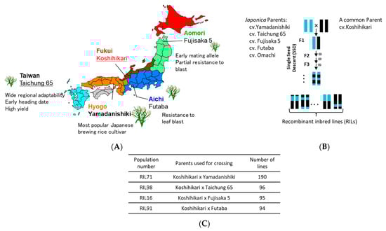
Figure 1.
(A) Origin of Japanese rice parents used for generating Japanese recombinant inbred lines (RILs). (B) A simplified crossing scheme using single seed descend method (SSD) to generate the four RIL populations used in this study and number of their corresponding progeny lines (C).
2.2. GRAS-Di Genotyping and Markers
Genotyping using GRAS-Di generated a total of 1050 (495 SNPs and 555 amplicons), 1285 (499 SNPs and 786 amplicons), 1708 (593 SNPs and 1115 amplicons), and 1704 (635 SNPs and 1069 amplicons) markers for RIL71, RIL98, RIL16, and RIL91, respectively (Supplementary Figure S2).
After the integration of all markers together, only one reliable marker was kept among a set of co-localized markers. Once the remaining co-localized markers were removed, we retained 527, 455, 501, and 436 markers for RIL71, RIL98, RIL16, and RIL91, respectively (Figure 2, Table 2). This suggested the location, on average, of one DNA marker every 700 kb, 820 kb, 744 kb, and 850 kb in RIL71, RIL98, RIL16, and RIL91, respectively (based on a genome size of Nipponbare reference sequence of approximately 373 Mb (IRGSP-1.0)). The integration map of all markers generated by both GoldenGate assay and GRAS-Di technology displayed a total of 1360, 1605, 2018, and 2056 markers for RIL71, RIL98, RIL16, and RIL91, respectively (Table 3).
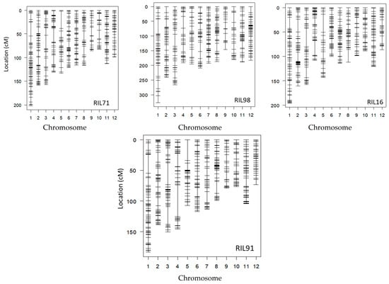
Figure 2.
Linkage maps of the four RIL populations based on the integration of both markers generated by GoldenGate system and GRAS-Di technology, excluding the co-localized markers.
Table 2.
Details on linkage maps of four RIL populations RIL71 (A), RIL98 (B), RIL16 (C) and RIL91 (D), integrating both markers generated by GoldenGate system and GRAS-Di technology, excluding the co-localized markers.
Table 3.
Details on integration linkage maps of four RIL populations RIL71 (A), RIL98 (B), RIL16 (C) and RIL91 (D) including both markers generated by GoldenGate system and GRAS-Di technology (including the co-localized markers).
The density of DNA markers, their distribution, and information on the integration linkage map for the four populations are summarized in Table 2. For RIL71, the total genome length is 1515 cM, including the above-mentioned 527 markers with unique map positions. The average distance between adjacent markers is 2.9 cM. Chromosome 7 is the most saturated, with an average distance of 2.3 cM. However, chromosome 5 is the least saturated, with an average distance of 4.7 cM. The longest chromosome is chromosome 1, with a total length of 202 cM, and the shortest is chromosome 10, with an average length of 81.7 cM. After excluding the co-localized markers, the integrated linkage map derived from genotyping of RIL98 population exhibits a total genome length of 1489 cM; the average distance between adjacent markers is 3.4 cM. Chromosome 1 is the longest, with an average length of 200.4 cM, and chromosome 9 the shortest one, with an average length of 90.4 cM. The most saturated chromosome is chromosome 7, with an average distance of 2.1 cM, whereas chromosome 10 is the less saturated, with an average distance 4.5 cM between markers. As for the integration map using RIL16 population, the full genome length is 1485.2 cM, and the average distance between adjacent markers is 3 cM. Chromosome 1 is the longest chromosome, with an average length of 195.7 cM, and chromosome 12 is the shortest one, with an average length of 86.3 cM. The most saturated chromosome is chromosome 6, with an average distance of 2.1 cM, and chromosome 3 is the least saturated, with an average distance 3.5 cM between markers. Integrated linkage map of RIL91 shows a full genome length of 1389.9 cM, with an average distance between adjacent markers of 3.4 cM. Chromosome 1 is the longest chromosome, with an average length of 183.6 cM, and chromosome 12 the shortest one, with an average length of 73.7 cM. The two densest chromosomes are chromosomes 11 and 12, with an average distances of 2.6 cM, whereas chromosome 4 contains the fewest markers, with an average distance of 4.7 between markers.
2.3. Genotyping by GoldenGate SNP Assay
In an attempt to confirm the increase of DNA marker information provided by GRAS-Di technology, we compared the linkage maps generated by GoldenGate assay with the integrated linkage maps generated by both GRAS-Di and GoldenGate assay (Figure 3 and Figure 4). The linkage map generated by GoldenGate assay provided a total of 292 markers in RIL71, 277 markers in RIL98, 262 markers in RIL16, and 286 markers in RIL91 (Table 4). The number of markers increased to 527 in RIL71 when we integrated makers generated by GRAS-Di and GoldenGate technologies together. Likewise, the integrated linkage maps from GRAS-Di and GoldenGate displayed a total of 455 markers in RIL98, 501 markers in RIL16, and 436 markers in RIL91 (Table 2).
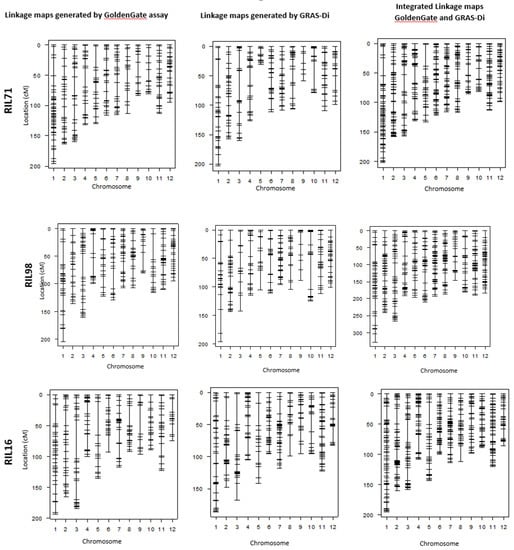
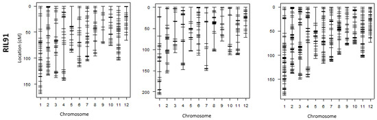
Figure 3.
Individual linkage maps generated by GoldenGate and GRAS-Di and their corresponding integrated maps using the four RIL populations.
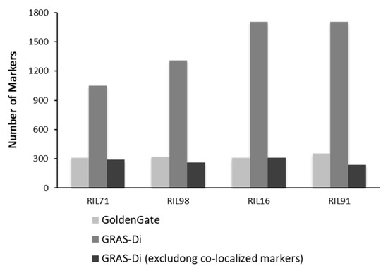
Figure 4.
Comparison of number of markers generated by GoldenGate assay (including the co-localized markers) and GRAS-Di (including and excluding the co-localized markers).
Table 4.
A linkage map created using markers obtained by the GoldenGate method, excluding the co-localized markers.
Although there is a difference in markers density among chromosomes, the total number of DNA markers witnessed a clear increase. In each chromosome, the average distance between markers decreased from 5.3 cM to 2.9 cM in the integrated linkage map of RIL71, from 5.5 cM to 3.4 cM when we integrated all markers using RIL98, from 5.8 cM to 3 cM in the integration map of RIL16, and from 4.8 cM to 3.4 cM in the integrated map of RIL91. Moreover, markers generated by both GoldenGate SNP assay and GRAS-Di were checked for their correspondence in the four populations. A corresponding ratio of 99.8% was observed within the four RIL populations (Supplementary Figure S3), indicating that all linkage maps generated by GRAS-Di have a good agreement with those generated by GoldenGate assay.
Comparison of chromosomal sections lacking DNA markers (hereinafter referred to as “the largest gap”) in both maps (i.e., linkage map generated after genotyping by GoldenGate assay vs. linkage map genotyping by GRAS-Di) showed that the largest gaps became narrower after GRAS-Di genotyping. For instance, these largest gaps have been narrowed by up to 13.7 cM in the linkage map generated using RIL71 population (Table 3 and Table 4). The genotyping by GRAS-Di yielded new markers in seven chromosomes (1, 2, 3, 4, 8, 9, and 11) within the largest gap section of the individual linkage map generated by GoldenGate assay. Consequently, the size of these largest gaps was narrowed by 0.3–6.7 cM in the integrated map. In chromosomes 6, 7, and 12, new DNA markers were generated between markers having the largest gap. In chromosome 7, for instance, nine new markers were added to the previous individual linkage map (GoldenGate) resulting in smaller gap size in the integrated map. The same tendency was observed in the four other linkage maps. In the linkage map generated by GRAS-Di using RIL98 population, the largest gaps also become smaller in six chromosomes (chromosomes 1, 3, 4, 6, 9, and 10), and a maximum decrease of 24.2 cM was observed in chromosome 10 (Table 3 and Table 4). Moreover, the genotyping by GRAS-Di allowed for the identification of more DNA markers within the largest gap regions (Figure 3); for instance, the gap in chromosome 7 was filled with new markers, and the main gap was reduced from 19.4 cM to 9 cM (Table 3 and Table 4).
Likewise, the largest gaps in linkage maps of RIL16 and RIL91 were narrowed in many chromosomes, and new DNA markers filled the gaps generated by GoldenGate SNP genotyping. A reduction in largest gaps was noted in chromosomes 8, 10, 11, and 12 of the linkage map generated by GRAS-Di using RIL16 population and in chromosomes 5, 6, 9, and 10 of the linkage map generated by GRAS-Di in RIL91 (Figure 3). It is worth mentioning that the reduction of the “largest gap” reached 34.6 cM in chromosome 9 in the individual linkage map of RIL16 population. The maximum decrease in gaps reached 11.5 cM in chromosome 9 of RIL91. On the other hand, we observed a slight increase in the “largest gaps” of some chromosomes following the genotyping by GRAS-Di; the genetic distance of the largest gaps in chromosomes 5 and 10 of the linkage map of RIL71 population, for instance, increased from 34.9 to 36.6 cM and 17.9 to 18.0 cM, respectively. This increase also affected the largest gaps of other linkage maps, such as in chromosomes 2, 5, 8, and 11 of RIL98 population, in chromosomes 2 and 4 (chromosome 2: an increase from 25.5 to 36.7 cM, chromosome 4: an increase from 25.8 to 29.4 cM) of RIL16, and a slight increase in chromosomes 1, 3, 4, and 8 for the linkage map of RIL91 population (Figure 3; Table 3 and Table 4). Ultimately, following GRAD-Di genotyping, largest gaps of integrated linkage maps generated in this study have a genetic distance of approximately 30 cM (chromosomes 1, 3, 4, and 5 in the linkage map of RIL71; chromosome 1 in the linkage map of RIL98; chromosomes 2, 3, 4, 5, and 8 in the linkage map of RIL 16; and chromosomes 1, 3, 4, and 5 in the linkage map of RIL91). In addition, the largest gap in chromosome 12 in the integration map generated from RIL98 population as well as chromosomes 1, 3, 4, and 8 in the map of RIL91 slightly increased (Table 3). The corresponding genetic position, however, appeared different from the one in the map generated following genotyping by GoldenGate assay (Table 4). When we looked to the genotype data, it appeared that the recombination frequency between the newly acquired DNA markers (generated by GRAS-Di technology) and the adjacent DNA markers was higher than the recombination in the same region (largest gap) generated by GoldenGate assay, which explains the slight increase in the largest gap following GRAS-Di technology.
2.4. Identification of QTLs for Heading Date
Heading date (Hd) is an important trait for adaptation and expansion of rice to different cultivation areas. QTLs analysis for Hd was performed using the above linkage maps. As shown in Figure 5, significant LOD scores over the thresholds indicated the presence of QTLs in three chromosomes: chromosomes 3, 6, and 7. Peaks of LOD scores in these chromosomal regions were confirmed to be involved in heading date trait using the linkage map data of four RIL populations (Figure 5). The QTLs for Hd6 and Hd16 were detected on chromosome 3 using the four integrated linkage maps generated in this study. Additionally, three more QTLs were detected in chromosome 6 (Hd1, using linkage maps of RIL16 and RIL98; and Hd17, using linkage map of RIL71) and chromosome 7 (Hd2, using linkage map of RIL91).
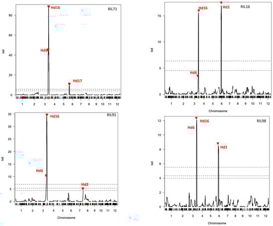
Figure 5.
QTL analysis of heading date in four rice RIL populations using integrated linkage maps generated by GRAD-Di and GoldenGate. The dashed lines indicate 1%, 5% (RIL71 and RIL16), and 10% (RIL91 and RIL98) of genome-empirical thresholds.
3. Discussion
Most Japanese rice cultivars are of japonica origin. Previous studies classified Japanese rice accessions into temperate and tropical japonica using simple sequence repeats (SSR) markers [33]. Also using SSR markers, a previous study [21], provided an estimation regarding the genetic diversity of Japanese rice cultivars and demonstrated the presence of population structure, revealing the presence of six subgroups and admixture in the Japanese rice population. However, despite the phenotypic variation reported in Japanese cultivars [33], its genetic dissection remained limited because of the lack of molecular markers allowing the detection of polymorphism. The first molecular linkage map from japonica × japonica cross was developed by Redona and Mackill [34] using random amplified polymorphic DNA (RAPD) and restriction fragment length polymorphism (RFLP) markers and succeeded in the detection of QTLs for seedling vigor. To generate their japonica map, the authors used F2 progeny derived from the cross between cv. Italica Livorno and cv. Labelle. They suggested that regions in chromosomes 1 and 2 might lack polymorphism in japonica cultivars in contrast to chromosomes 10 and 11, which might be highly polymorphic among temperate and tropical group of japonica subspecies. Recent advances in genotyping technologies and associated reduced costs has changed the way to detect genome-wide polymorphism, since SNPs already replaced SSRs as the first DNA marker of choice [35]. These SNPs could be used to detect further DNA polymorphism among closely related cultivars; for instance, Yamamoto et al. [11] used whole genome sequencing of two closely related japonica rice cultivars, Koshihikari and Nipponbare, and collected over 67,000 SNPs between them. Subsequently, Nagasaki and collaborators [36] compared the genomic sequence of two other japonica cultivars (Eiko and Rikuu132) and Nipponbare as reference to construct a core set of 768 SNPs highly efficient and reliable for diversity and genetic analysis of biparental populations of Japanese rice accessions.
In the present study, Koshihikari cv. was used as a common parent to generate four RIL populations: Yamadanishiki is popular for its highest yielding and excellent brewing quality, which made it a good candidate as a crossing parent to conduct QTL analysis [31]. Taichung 65 is a japonica cultivar derived from the cross between Kameji and Shinriki; its potential for breeding includes early heading date (valuable trait for wide regional adaptability) and high yield [37]. Cultivars Fujisaka 5 and Futaba are, however, renamed mainly for their partial and higher resistance to leaf blast [29,30]. Over the generations, by crossing each of these four Japanese parent cultivars with Koshihikari cultivar, the final genotype of the generated RILs was a random shuffle of parental genotypes. Since each self-pollination reduces heterozygosity by half, the majority of genomes of RILs have become homozygous at advanced generations (F6–F7). Then, in order to reveal potential hidden polymorphism among Japanese rice cultivars, we used GRAS-Di technology to sequence and genotype these four RIL populations and their respective parents. The low cost and high accuracy of GRAS-Di allowed an accurate sequencing using 1× genome coverage of the four RIL populations and their respective parents (Table 1). GRAS-Di technology has randomly amplified multiple regions of the genome to generate amplicons that have been subjected to NGS sequencing [12]. Additionally, GRAS-Di genotyping of the F6-F7 of the four RIL populations and their respective parents confirmed that these populations were almost fixed to the homozygous state (data not shown) and generated a considerable number of markers used to display genetic linkage maps using data of four RIL populations. The total number of markers generated by GRAS-Di (amplicon and SNP markers) was compared with the number of SNP markers previously generated by GoldenGate assay. Although there was a difference in markers density between chromosomes, the total number of DNA markers witnessed a clear increase (Table 4). The distribution of DNA markers, however, is not uniform across the four linkage maps. Gaps between markers were localized in different chromosomes of the four linkage maps (Figure 2 and Figure 3). This uneven distribution of markers might be related to the low frequency of DNA polymorphism in these particular genomic regions, for instance, between Koshihikari and Yamadanishiki for individuals of RIL71 population, Koshihikari and Taichung 65 for individuals of RIL98 population, Koshihikari and Fujisaka5 for individuals of RIL16, and Koshihikari and Futaba for individuals of RIL91 population.
However, in this study, chromosomal regions displaying “SNP deserts” (term defined in [38]), such as in chromosome 5, and which have been related to rice domestication, have been relatively filled with markers in the integrated linkage map of RIL98 (Figure 3). The same region on chromosome 5 appeared empty of markers in the three remaining linkage maps derived from RIL71, RIL16, and RIL91. Moreover, a lower recombination rate around the centromere could also explain the reason of this distorted recombination and the low frequency of markers around these regions of the genome.
Overall, the average genetic distance between markers decreased in the four integrated linkage maps (Figure 3), but the total chromosome length did not significantly change when we compared displayed linkage maps using GoldenGate SNP markers and GRAS-Di markers. Consequently, the integrated maps provided higher density level of arranged markers. The corresponding ratio of 99.8% observed within the four RIL populations indicated that all linkage maps generated by GRAS-Di have a good agreement with those generated by GoldenGate assay. The comparison of largest gaps displayed in linkage maps generated by GoldenGate assay and GRAS-Di, showed a general narrowing of these gaps following the use of GRAS-Di, and this was due to generation of new markers within the largest gap regions. For instance, new markers were generated in seven chromosomes of the linkage map displayed when using RIL71 population, allowing a narrowing of up to 6.7 cM when we integrated both maps (Table 3 and Table 4). In the individual linkage map using RIL98, chromosome 7 witnessed a shrinkage of more than 10 cM following GRAS-Di genotyping. The reduction of the “largest gap” reached 34.6 cM in chromosome 9 in the individual linkage map of RIL16 population. Despite this general decrease in the largest gaps generated by GRAS-Di genotyping, we observed a slight increase of these largest gaps in some chromosomes (Figure 3, Table 3 and Table 4). Since the corresponding markers were in the same position as in linkage maps of GoldenGate assay, this slight increase was considered as a potential error of calculation. In some other chromosomal gap regions, despite the presence of additional markers incorporated after GRAS-Di genotyping, the largest gap did not much change, this is because the new markers are closely located to markers obtained by the GoldenGate assay.
Yamamoto and collaborators [11] sequenced the leading Japanese variety Koshihikari and found fewer SNP regions (compared with Nipponbare reference sequence) in chromosomes 5, 6, and 9, resulting in SNP gaps [36]. This was explained by the absence of DNA polymorphism between Koshihikari and Nipponbare because of the share of common chromosome segments on both genomes. This might also explain the absence of DNA polymorphism between Koshihikari and Yamadanishiki, Koshihikari and Taichung 65, Koshihikari and Fujisaka 5, and Koshihikari and Futaba [36]. However, in the present study, DNA polymorphisms were detected by NGS, which revealed a high possibility of DNA polymorphisms in regions where no DNA markers were obtained before.
Climate change and the unpredictable performance (for example, heading date and grain yield) of cereal crops are of increasing concern. Japanese rice population, which originated from closely related cultivars, has a narrow genetic diversity, which hampered previous temptations to perform genetic dissection of phenotypic variations observed among Japanese rice cultivars. To identify candidate genes or QTLs responsible for the phenotypic and performances differences between Japanese rice cultivars, we constructed RILs among four Japanese rice and Koshihikari cultivars, which are genetically close.
The present study used a recently developed method for genotyping by sequencing “GRAS-Di”, which was highly effective and could identify a large number of genetic markers despite the lack of DNA polymorphism between the used parent lines. The integration of markers generated by GRAS-Di and a previously generated GoldenGate SNP markers produced a higher density linkage map with significantly reduced average distance between markers. In addition to these genotyping data, the same RILs were used to assess several phenotypical traits, such as those related to the heading date. The combination of these phenotyping with the genotyping data generated by GRAS-Di allowed for the efficient mapping of QTLs controlling heading date in Japanese rice. Interestingly, the position of Hd6 and Hd16, corresponding to two previously reported QTLs in chromosome 3 [24,39], was consistently confirmed in this study using all linkage maps generated by GRAS-Di. Likewise, the positions of three other QTLs reported in this study were also previously reported as QTLs located at the top and the middle of chromosome 6 (Hd17 and Hd1, respectively) [40,41] and the end of chromosome 7 (Hd2, [42]). This result demonstrates that major QTLs for heading date, previously reported, could be successfully confirmed using linkage maps generated by GRAS-Di genotyping platform.
4. Materials and Methods
4.1. Plant Material and DNA Isolation
Four recombinant inbred lines (RIL71, RIL98, RIL16, and RIL91) of O. sativa subsp. japonica, developed from independent crosses of cultivars Yamadanishiki, Taichung 65, Fujisaka 5, and Futaba, respectively, with the common cultivar Koshihikari, were used in this study. The obtained F1 progeny was self-fertilized to produce F2 progeny. Each of the F2 was brought to F7 generation by a single seed descent (SSD) method to generate a final progeny number of 190, 96, 95, and 94 for RIL 71, RIL98, RIL16, and RIL91, respectively (Figure 1). These populations were developed in the experimental field at the Food Resources Education and Research Center, Graduate School of Agricultural Science, Kobe University, Kasai City, Hyogo Prefecture, Japan. Bulked leaf samples from each of the four RILs populations (F7 generation) and their respective parents were collected from one-month-old seedlings, dried overnight at 50 °C, and used for total genomic DNA extraction using CTAB [43] protocol with slight modifications.
4.2. DNA Sequencing and Genotyping
We used genotyping by random amplicon sequencing-direct (GRAD-Di) technology for sequencing and genotyping the four RIL populations and their respective parents. GRAS-Di has been recently developed by Toyota Motor Corporation [12] and licensed to Eurofins Genomics. This technology allows for the amplification of multiple parts of the genome by performing two rounds of PCR with high concentration of random primers and adapter sequences to generate a sequence library of tens of thousands of amplicons (Supplementary Figure S1A). GRAS-Di PCR first used a high concentration of random primers (Supplementary Table S1), with Nextera adaptor sequences and 3-base random oligomers that randomly bind to genomic DNA to amplify nonspecific regions of the entire genome. The second PCR is used for indexing and includes Illumina multiplexing 8-base dual index and P7/P5 adapter sequence (Supplementary Table S2). The final genome-wide amplified amplicons were pooled and purified for sequencing using either HiSeq2500 NGS-platforms (Illumina, Inc., San Diego, CA, USA) to generate paired-end reads ranging from 100 to 150 bp depending on the sequence platform (main steps for genotyping and construction of linkage maps are summarized in Supplementary Figure S1B). Construction of library and sequencing of the amplicons were carried out by Eurofins Genomics (Supplementary Figure S1A). To determine the optimal coverage to be used for efficient sequencing and to obtain as many SNP markers as possible, we performed a first sequencing trial of RIL71 using two independent replications of the same library (95 lines). When the sequence depth was 1× the genome, the number of obtained markers was 1089. However, when the depth increased to 2×the genome, the number of markers did not improve much (only 1792 markers were generated), which suggested that 1× sequencing depth should be adequate to detect SNP markers distributed throughout the genome.
For SNP and amplicons marker detection, adapter sequences were removed using cutadapt (ver.1.16) company software. Trimmed reads were mapped to Nipponbare (IRGSP-1.0) reference sequence using Bowtie2 (ver.2.3.3.1) software. For the detection of SNP markers, sequence bases that were different from the Nipponbare reference were extracted using samtools (ver.1.6)/bcftools (ver.1.6) and SNP mutations filtered using vcftools. Further filtering using beagle (ver.4.0) software was performed to ultimately keep only reliable mutations that enable detection of polymorphism between RILs and their corresponding parents. For convenience, SNPs were named on the basis of their physical locations (SNP/chromosome number/physical position). For amplicon markers detection, the polymorphism was judged on the basis of the presence or absence of a particular sequence read in the genome of both parents (i.e., the presence of a sequence in one parent genome and absence in the second parent genome). Once defined as a reliable amplicon marker to be used for genotyping, each RILs population was genotyped on the basis of the presence or absence of the read, and the genomic position of the amplicon marker was determined using the “Nipponbare” (IRGSP-1.0) reference sequence. The analysis of the obtained results was characterized by high reproducibility of amplicon amplification and a minimal loss of genotype data. Amplicon markers were named as follows: AMP/chromosome number/physical position.
SNP marker identification and genotyping using GoldenGate assay were performed using procedures described by Yamamoto and collaborators [11]. Candidate SNPs between Nipponbare and Koshihikari genome sequences were selected at a spacing of 100 to 200 kb and used for genotyping. SNP adaptability to the Illumina (San Diego, CA, USA) GoldenGate detection system was scored using the Illumina online scoring system (http://icom.illumina.com). SNPs with a score higher than 0.4 were selected to design 768-plex SNPs for Illumina GoldenGate BeadArray technology platform [11]. A total of 151 representative Japanese rice cultivars subsp japonica, including Yamadanishiki, Taichung 65, Fujisaka 5, and Futaba, which have been grown during the past 150 years, were used for SNP array analysis. Total DNA from parents of four RIL populations was extracted, and 5µL of 50 ng/µL DNA was used for SNP analysis. Data processing and bioinformatics analysis were conducted by Eurofin Genomics. To check the coherence between markers obtained by GoldenGate and GRAS-Di genotyping, the same genomic regions of all markers obtained by GoldenGate and GRAS-Di were compared on the basis of a threshold of 50 kb distance between GoldenGate-SNP and GRAS-Di-amplicon, or GoldenGate-SNP and GRAS-Di-SNP. Red cell color for each DNA marker corresponds to the genomic region of Koshihikari (A) and green cell color corresponds to the founder genotype (B). As shown in the tables of Supplementary Figure S3, almost all markers detected by GoldenGate and having A or B genotypes have been confirmed with the same genotype using GRAS-Di technology. The corresponding ratio is the quotient of the sum of markers having the same genotype regardless of the genotyping method to the total number of markers generated by GRAS-DI technology.
4.3. Linkage Map Construction
Following the alignment of sequence reads to the Nipponbare (IRGSP-1.0 [44]) reference sequence and after filtering SNPs and sorting them according to their genomic position, a quality control of the genotyping data was performed to exclude any possible alignment errors. Markers showing only Koshihikari or second parent founder homozygous or heterozygous genotypes were discarded. Too many heterozygous markers were also excluded from the analysis. Physically closely located markers that still show recombination are unlikely to be true markers and, thus, were excluded from the analysis. Ambiguous genotypes, for instance, ambiguous amplicon markers mapped to Nipponbare reference sequence with low read count, were converted to missing genotypes codes NA (not applicable) or “-“. Within a set of co-localized markers, only one reliable marker was kept, and other co-localized markers were discarded. SNP markers confirmed with a ratio of 1:1 (Koshihikari:Founder) were used to construct the genetic linkage map. Kosambi’s mapping function was used to convert the recombination frequency to a genetic map distance [45]. The R package R/qtl was used to display the linkage map [46].
4.4. Evaluation of Phenotypic Data and QTL Analysis
In 2021, the four RIL populations and their parents were sown from April 26th to 28th. Six plants per line were transplanted to the experimental field at Kobe University, Food Resources Education and Research Center (Kasai City, Hyogo Prefecture, Japan; 34.88 N, 134.86 E) between June 1st and June 2nd of the same year. The evaluation of days to heading was conducted on six plants per line. QTL analysis was performed using linkage maps derived from the four RIL populations using the R package R/qtl [46]. Detection of QTLs was carried out using the composite interval mapping method [47] with a setting of window size and walk speed of 3 and 1 cM, respectively. The empirical threshold logarithm of odds (LOD) values were determined by computing 1000 permutations [48]. Confidence intervals were calculated from the 1-LOD support interval.
Supplementary Materials
The following supporting information can be downloaded at: https://www.mdpi.com/article/10.3390/plants12040929/s1, Figure S1. (A) Scheme summarizing the main steps for GRAS-Di library construction in this work. (B) Flow chart of main steps adopted for genotyping analysis and linkage mapping; Table S1. Primer sequences for the first PCR; Table S2. Primer sequences for the second PCR; Figure S2: Total number of markers generated by GRAS-Di; Figure S3: Example of calculation of correspondence ratio between makers generated by GoldenGate method and markers generated by GRAS-Di technology.
Author Contributions
Conceptualization, M.Y. and R.F.; methodology, H.E., M.Y., T.O., R.M., K.S. and M.I.; formal analysis, R.F, Y.I., S.O., M.M. and M.Y; investigation, M.Y., R.M. and R.F.; resources, M.Y.; data curation, Y.I., R.F. and M.Y.; writing—original draft preparation, R.F.; writing—review and editing, all authors; supervision, M.Y.; project administration, M.Y.; funding acquisition, M.Y. All authors have read and agreed to the published version of the manuscript.
Funding
This research was funded by the Japan Science and Technology Agency (JST) CREST Grant Number JPMJCR17O3 and Cross-ministerial Strategic Innovation Promotion Program (SIP) “Technologies for creating next-generation agriculture, forestry and fisheries” (funding agency: Biooriented Technology Research Advancement Institute, NARO).
Data Availability Statement
Not applicable.
Acknowledgments
We thank Najla Mezghani and Sophien Kamoun for suggestions to improve the manuscript.
Conflicts of Interest
The authors declare no conflict of interest. The funders had no role in the design of the study; in the collection, analyses, or interpretation of data; in the writing of the manuscript; or in the decision to publish the results.
References
- Jiang, W.; Struik, P.C.; Lingna, J.; Van Keulen, H.; Ming, Z.; Stomph, T.J. Uptake and distribution of root-applied or foliar-applied 65Zn after flowering in aerobic rice. Ann. Appl. Biol. 2007, 150, 383–391. [Google Scholar] [CrossRef]
- Ahn, S.; Anderson, J.A.; Sorrells, M.E.; Tanksley, S.D. Homoeologous relationships of rice, wheat and maize chromosomes. Mol. Gen. Genet. 1993, 241, 483–490. [Google Scholar] [CrossRef]
- Kurata, N.; Moore, G.; Nagamura, Y.; Foote, T.; Yano, M.; Minobe, Y.; Gale, M. Conservation of genome structure between rice and wheat. Nat. Biotechnol. 1994, 12, 276–278. [Google Scholar] [CrossRef]
- Buell, C.R.; Yuan, Q.; Ouyang, S.; Liu, J.; Zhu, W.; Wang, A.; Maiti, R.; Haas, B.; Wortman, J.; Pertea, M.; et al. Sequence, annotation, and analysis of synteny between rice chromosome 3 and diverged grass species. Genome Res. 2005, 15, 1284–1291. [Google Scholar] [CrossRef] [PubMed]
- Goff, S.A.; Ricke, D.; Lan, T.-H.; Presting, G.; Wang, R.; Dunn, M.; Glazebrook, J.; Sessions, A.; Oeller, P.; Varma, H.; et al. A draft sequence of the rice genome (Oryza sativa L. ssp. japonica). Science 2002, 296, 92–100. [Google Scholar] [CrossRef]
- Yu, J.; Hu, S.; Wang, J.; Wong, G.K.S.; Li, S.; Liu, B.; Deng, Y.; Dai, L.; Zhou, Y.; Zhang, X.; et al. A draft sequence of the rice genome (Oryza sativa L. ssp. indica). Science 2002, 296, 79–92. [Google Scholar] [CrossRef]
- Abe, A.; Kosugi, S.; Yoshida, K.; Natsume, S.; Takagi, H.; Kanzaki, H.; Matsumura, H.; Yoshida, K.; Mitsuoka, C.; Tamiru, M.; et al. Genome sequencing reveals agronomically important loci in rice using MutMap. Nat Biotechnol. 2012, 30, 174–178. [Google Scholar] [CrossRef]
- Fekih, R.; Takagi, H.; Tamiru, M.; Abe, A.; Natsume, S.; Yaegashi, H.; Sharma, S.; Sharma, S.; Kanzaki, H.; Matsumura, H.; et al. MutMap+: Genetic mapping and mutant identification without crossing in rice. PLoS ONE 2013, 8, e68529. [Google Scholar] [CrossRef]
- Takagi, H.; Abe, A.; Yoshida, K.; Kosugi, S.; Natsume, S.; Mitsuoka, C.; Uemura, A.; Utsushi, H.; Tamiru, M.; Takuno, S.; et al. QTL-seq: Rapid mapping of quantitative trait loci in rice by whole genome resequencing of DNA from two bulked populations. Plant J. 2013, 74, 174–183. [Google Scholar] [CrossRef]
- Varshney, R.K.; Terauchi, R.; McCouch, S.R. Harvesting the promising fruits of genomics: Applying genome sequencing technologies to crop breeding. PLoS Biol. 2014, 12, e1001883. [Google Scholar] [CrossRef]
- Yamamoto, T.; Nagasaki, H.; Yonemaru, J.-I.; Ebana, K.; Nakajima, M.; Shibaya, T.; Yano, M. Fine definition of the pedigree haplotypes of closely related rice cultivars by means of genome-wide discovery of single-nucleotide polymorphisms. BMC Genom. 2010, 11, 267. [Google Scholar] [CrossRef] [PubMed]
- Enoki, H.; Takeuchi, Y. New genotyping technology, GRAS-Di, using next generation sequencer. In Proceedings of the Plant and Animal genome conference XXVI, San Diego, CA, USA, 13–17 January 2018; Available online: https://pag.confex.com/pag/xxvi/meetingapp.cgi/Paper/29067 (accessed on 10 January 2023).
- Hosoya, S.; Hirase, S.; Kikuchi, K.; Nanjo, K.; Nakamura, Y.; Kohno, H.; Sano, M. Random PCR-based genotyping by sequencing technology GRAS-Di (genotyping by random amplicon sequencing-direct) reveals genetic structure of mangrove fishes. Mol. Ecol. Resour. 2019, 19, 1153–1163. [Google Scholar] [CrossRef] [PubMed]
- Enoki, H. The construction of pseudomolecules of a commercial strawberry by DeNovoMAGIC and new genotyping technology, GRAS-Di. In Proceedings of the Plant and Animal genome conference XXVII, San Diego, CA, USA, 12–16 January 2019; Available online: https://pag.confex.com/pag/xxvii/meetingapp.cgi/Paper/37002 (accessed on 10 January 2023).
- Zhang, Q.; Maroof, M.A.S.; Lu, T.Y.; Shen, B.Z. Genetic diversity and differentiation of indica and japonica rice detected by RFLP analysis. Theor. Appl. Genet. 1992, 83, 495–499. [Google Scholar] [CrossRef] [PubMed]
- Gupta, P.K.; Rustgi, S.; Kulwal, P.L. Linkage disequilibrium and association studies in higher plants: Present status and prospects. Plant Mol. Biol. 2005, 57, 461–485. [Google Scholar] [CrossRef] [PubMed]
- Terauchi, R.; Abe, A.; Takagi, H.; Tamiru, M.; Fekih, R.; Natsume, S.; Yaegashi, H.; Kosugi, S.; Kanzaki, H.; Matsumura, H.; et al. Whole genome sequencing to identify genes and QTL in rice. In Advances in the Understanding of Biological Sciences Using Next Generation Sequencing (NGS) Approaches; Springer: Berlin/Heidelberg, Germany, 2015; pp. 33–42. ISBN 9783319171579. [Google Scholar]
- Fekih, R.; Tamiru, M.; Kanzaki, H.; Abe, A.; Yoshida, K.; Kanzaki, E.; Saitoh, H.; Takagi, H.; Natsume, S.; Undan, J.R.; et al. The rice (Oryza sativa L.) LESION MIMIC RESEMBLING, which encodes an AAA-type ATPase, is implicated in defense response. Mol. Genet. Genom. 2015, 290, 611–622. [Google Scholar] [CrossRef]
- Nagata, K.; Ando, T.; Nonoue, Y.; Mizubayashi, T.; Kitazawa, N.; Shomura, A.; Matsubara, K.; Ono, N.; Mizobuchi, R.; Shibaya, T.; et al. Advanced backcross QTL analysis reveals complicated genetic control of rice grain shape in a japonica × indica cross. Breed. Sci. 2015, 65, 308–318. [Google Scholar] [CrossRef]
- Tamiru, M.; Takagi, H.; Abe, A.; Yokota, T.; Kanzaki, H.; Okamoto, H.; Saitoh, H.; Takahashi, H.; Fujisaki, K.; Oikawa, K.; et al. A chloroplast-localized protein lesion and lamina bending affects defence and growth responses in rice. New Phytol. 2016, 210, 1282–1297. [Google Scholar] [CrossRef]
- Yamasaki, M.; Ideta, O. Population structure in Japanese rice population. Breed Sci. 2013, 63, 49–57. [Google Scholar] [CrossRef]
- Yokoo, M.; Hirao, M.; Imai, T. Annual change in leading rice varieties between 1956 and 2000 in Japan. Bull. Natl. Inst. Crop Sci. 2005, 7, 19–125. [Google Scholar]
- Kobayashi, A.; Hori, K.; Yamamoto, T.; Yano, M. Koshihikari: A premium short-grain rice cultivar - its expansion and breeding in Japan. Rice 2018, 11, 15. [Google Scholar] [CrossRef]
- Hori, K.; Ogiso-Tanaka, E.; Matsubara, K.; Yamanouchi, U.; Ebana, K.; Yano, M. Hd16, a gene for casein kinase I, is involved in the control of rice flowering time by modulating the day-length response. Plant J. 2013, 76, 36–46. [Google Scholar] [CrossRef] [PubMed]
- Yu, J.; Holland, J.B.; McMullen, M.D.; Buckler, E.S. Genetic design and statistical power of nested association mapping in maize. Genetics 2008, 178, 539–551. [Google Scholar] [CrossRef] [PubMed]
- McMullen, M.D.; Kresovich, S.; Villeda, H.S.; Bradbury, P.; Li, H.; Sun, Q.; Flint-Garcia, S.; Thornsberry, J.; Acharya, C.; Bottoms, C.; et al. Genetic properties of the maize nested association mapping population. Science 2009, 325, 737–740. [Google Scholar] [CrossRef] [PubMed]
- Bajgain, P.; Rouse, M.N.; Tsilo, T.J.; Macharia, G.K.; Bhavani, S.; Jin, Y.; Anderson, J.A. Nested association mapping of stem rust resistance in wheat using genotyping by sequencing. PLoS ONE 2016, 11, e0155760. [Google Scholar] [CrossRef]
- Maurer, A.; Draba, V.; Jiang, Y.; Schnaithmann, F.; Sharma, R.; Schumann, E.; Kilian, B.; Reif, J.C.; Pillen, K. Modelling the genetic architecture of flowering time control in barley through nested association mapping. BMC Genom. 2015, 16, 290. [Google Scholar] [CrossRef]
- Takita, T.; Solis, R.O. Rice Breeding at the National Agricultural Research Center for the Tohoku Region (NARCT) and Rice Varietal Recommendation Process in Japan. Bull. Natl. Agric. Res. Cent. Tohoku Reg. 2002, 100, 93–117. (in Japanese). [Google Scholar]
- Saka, N. A Rice (Oryza sativa L.) Breeding for Field Resistance to Blast Disease (Pyricularia oryzae) in Mountainous Region Agricultural Research Institute, Aichi Agricultural Research Center of Japan. Plant Prod. Sci. 2006, 9, 3–9. [Google Scholar] [CrossRef]
- Okada, S.; Suehiro, M.; Ebana, K.; Hori, K.; Onogi, A.; Iwata, H.; Yamasaki, M. Genetic dissection of grain traits in Yamadanishiki, an excellent sake-brewing rice cultivar. Theor. Appl. Genet. 2017, 130, 2567–2585. [Google Scholar] [CrossRef]
- Inoue, H.; Nishida, H.; Okumoto, Y.; Tanisaka, T. Identification of an early heading time gene found in the Taiwanese rice cultivar Taichung 65. Breed. Sci. 1998, 48, 103–108. [Google Scholar] [CrossRef]
- Ebana, K.; Kojima, Y.; Fukuoka, S.; Nagamine, T.; Kawase, M. Development of mini core collection of Japanese rice landrace. Breed. Sci. 2008, 58, 281–291. [Google Scholar] [CrossRef]
- Redoña, E.D.; Mackill, D.J. Mapping quantitative trait loci for seedling vigor in rice using RFLPs. Theoret. Appl. Genet. 1996, 92, 395–402. [Google Scholar] [CrossRef] [PubMed]
- McCouch, S.R.; Zhao, K.; Wright, M.; Tung, C.-W.; Ebana, K.; Thomson, M.; Reynolds, A.; Wang, D.; DeClerck, G.; Ali, L.; et al. Development of genome-wide SNP assays for rice. Breed. Sci. 2010, 60, 524–535. [Google Scholar] [CrossRef]
- Nagasaki, H.; Ebana, K.; Shibaya, T.; Yonemaru, J.I.; Yano, M. Core single-nucleotide polymorphism —A tool for genetic analysis of the Japanese rice populationn. Breed. Sci. 2010, 60, 648–655. [Google Scholar] [CrossRef]
- Okumoto, Y.; Yoshimura, A.; Tanisaka, T.; Yamagata, H. Analysis of a rice variety Taichung 65 and its Isogenic early-heading lines for late-heading genes E1, E2 and E3. Jpn. J. Breed. 1992, 42, 415–429, (in Japanese with English summary). [Google Scholar] [CrossRef]
- Wang, L.; Hao, L.; Li, X.; Hu, S.; Ge, S.; Yu, J. SNP deserts of Asian cultivated rice: Genomic regions under domestication. J. Evol. Biol. 2009, 22, 751–761. [Google Scholar] [CrossRef] [PubMed]
- Takahashi, Y.; Shomura, A.; Sasaki, T.; Yano, M. Hd6, a rice quantitative trait locus involved in photoperiod sensitivity, encodes the alpha subunit of protein kinase CK2. Proc. Natl. Acad. Sci. USA 2001, 98, 7922–7927. [Google Scholar] [CrossRef]
- Matsubara, K.; Kono, I.; Hori, K.; Nonoue, Y.; Ono, N.; Shomura, A.; Mizubayashi, T.; Yamamoto, S.; Yamanouchi, U.; Shirasawa, K.A.; et al. Novel QTLs for photoperiodic flowering revealed by using reciprocal backcross inbred lines from crosses between japonica rice cultivars. Theor. Appl. Genet. 2008, 117, 935–945. [Google Scholar] [CrossRef]
- Yano, M.; Katayose, Y.; Ashikari, M.; Yamanouchi, U.; Monna, L.; Fuse, T.; Baba, T.; Yamamoto, K.; Umehara, Y.; Nagamura, Y.; et al. Hd1, a major photoperiod sensitivity quantitative trait locus in rice, is closely related to the Arabidopsis flowering time gene CONSTANS. Plant Cell. 2000, 12, 2473–2484. [Google Scholar] [CrossRef]
- Yano, M.; Harushima, Y.; Nagamura, Y.; Kurata, N.; Minobe, Y.; Sasaki, T. Identification of quantitative trait loci controlling heading date in rice using a high-density linkage map. Theor. Appl. Genet. 1997, 95, 1025–1032. [Google Scholar] [CrossRef]
- Doyle, J.J.; Doyle, J.J. A rapid procedure for DNA purification from small quantities of fresh leaf tissue. Phytochem. Bull. 1987, 19, 11–15. [Google Scholar]
- International Rice Genome Sequencing Project. The map-based sequence of the rice genome. Nature 2005, 436, 793–800. [Google Scholar] [CrossRef]
- Kosambi, D.D. The estimation of map distances from recombination values. Ann. Hum. Genet. 1943, 12, 172–175. [Google Scholar] [CrossRef]
- Broman, K.W.; Wu, H.; Sen, Ś.; Churchill, G.A. R/qtl: QTL mapping in experimental crosses. Bioinformatics 2003, 19, 889–890. [Google Scholar] [PubMed]
- Zeng, Z.B. A composite interval mapping method for locating multiple QTLs. In Proceedings of the 5th World Congress on Genetics Applied to Livestock Production, Guelph, ON, Canada, 7–12 August 1994; University of Guelph: Guelph, ON, Canada, 1994; Volume 7. [Google Scholar]
- Churchill, G.A.; Doerge, R.W. Empirical threshold values for quantitative trait mapping. Genetics 1994, 138, 963–971. [Google Scholar] [CrossRef]


Disclaimer/Publisher’s Note: The statements, opinions and data contained in all publications are solely those of the individual author(s) and contributor(s) and not of MDPI and/or the editor(s). MDPI and/or the editor(s) disclaim responsibility for any injury to people or property resulting from any ideas, methods, instructions or products referred to in the content. |
© 2023 by the authors. Licensee MDPI, Basel, Switzerland. This article is an open access article distributed under the terms and conditions of the Creative Commons Attribution (CC BY) license (https://creativecommons.org/licenses/by/4.0/).