
AMMI and GGE Biplot Analyses for Mega-Environment Identification and Selection of Some High-Yielding Oat (Avena sativa L.) Genotypes for Multiple Environments

 , , , , ,
Abstract
:1. Introduction
2. Results and Discussion
2.1. AMMI ANOVA
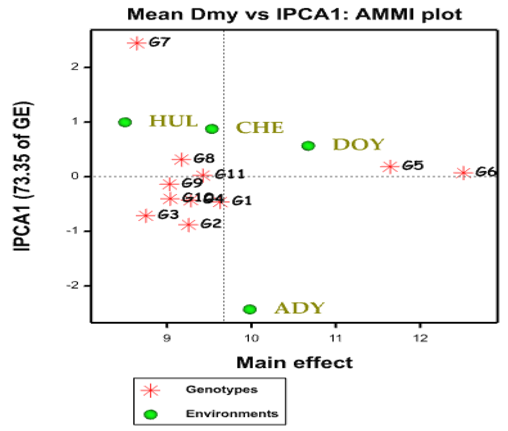
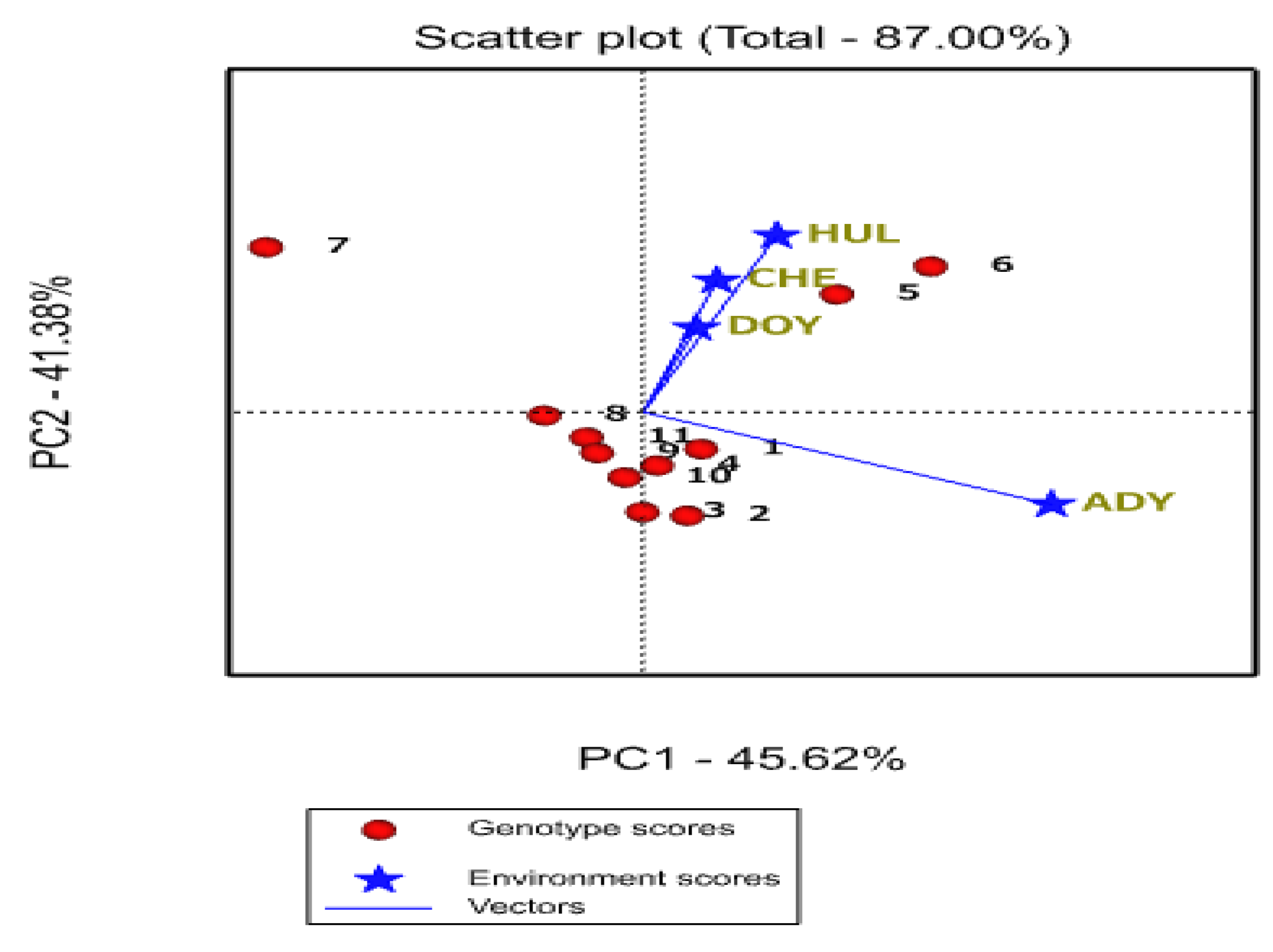
2.2. AMMI Biplot
2.3. AMMI Stability Value (ASV)
2.4. Genotype Selection Index (GSI) Analysis
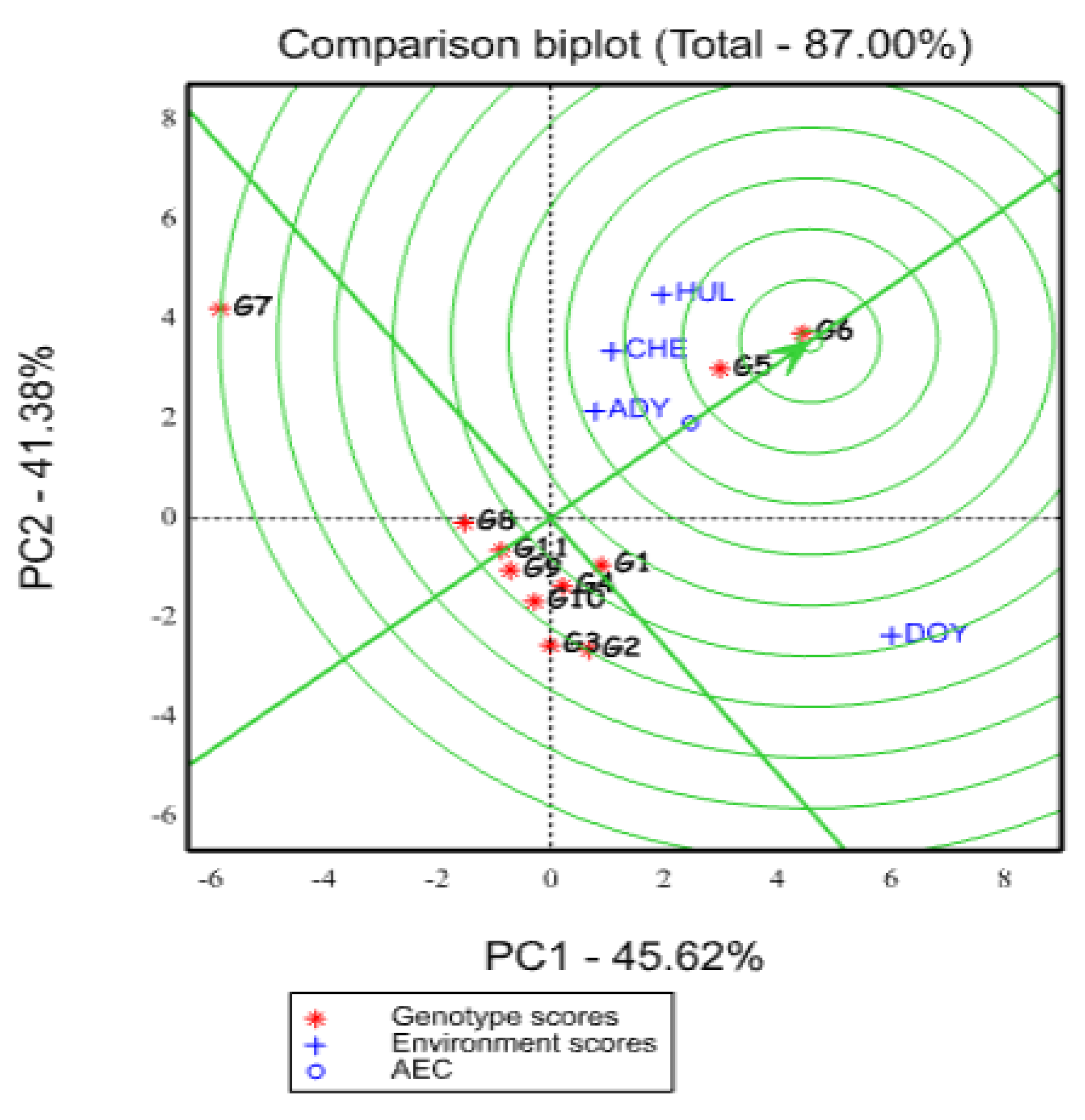
2.5. GGE Biplot
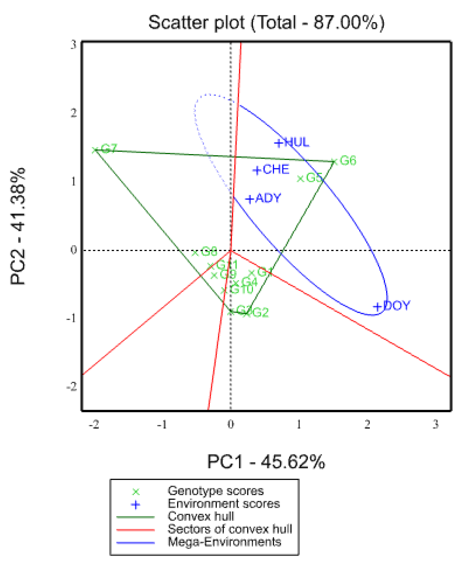
2.5.1. Which-Won-Where View of GGE Biplot
2.5.2. Relationship among Environments
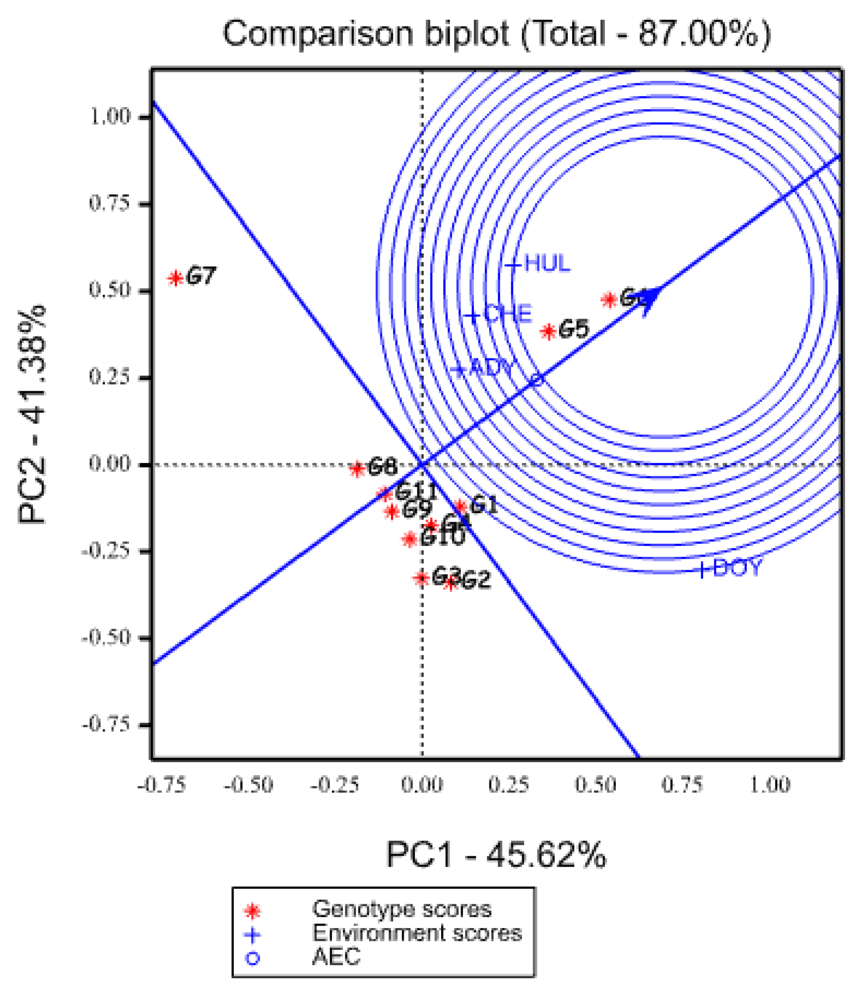
2.5.3. Evaluation of Genotypes Based on the Ideal Genotype
2.5.4. Evaluation of Environments Relative to Ideal Environments
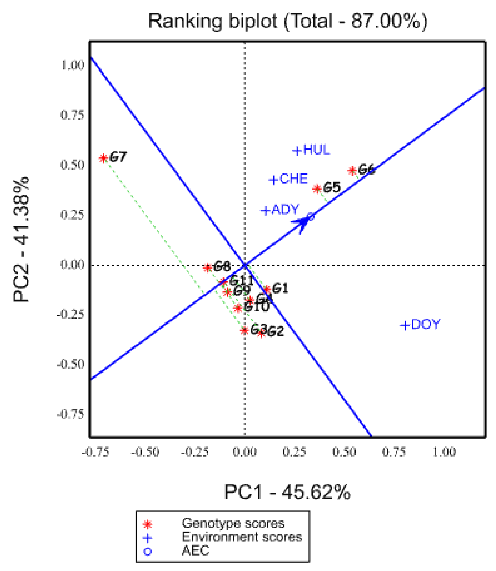
2.5.5. Ranking of Genotypes Based on Mean Yield and Stability Performance
3. Materials and Methods
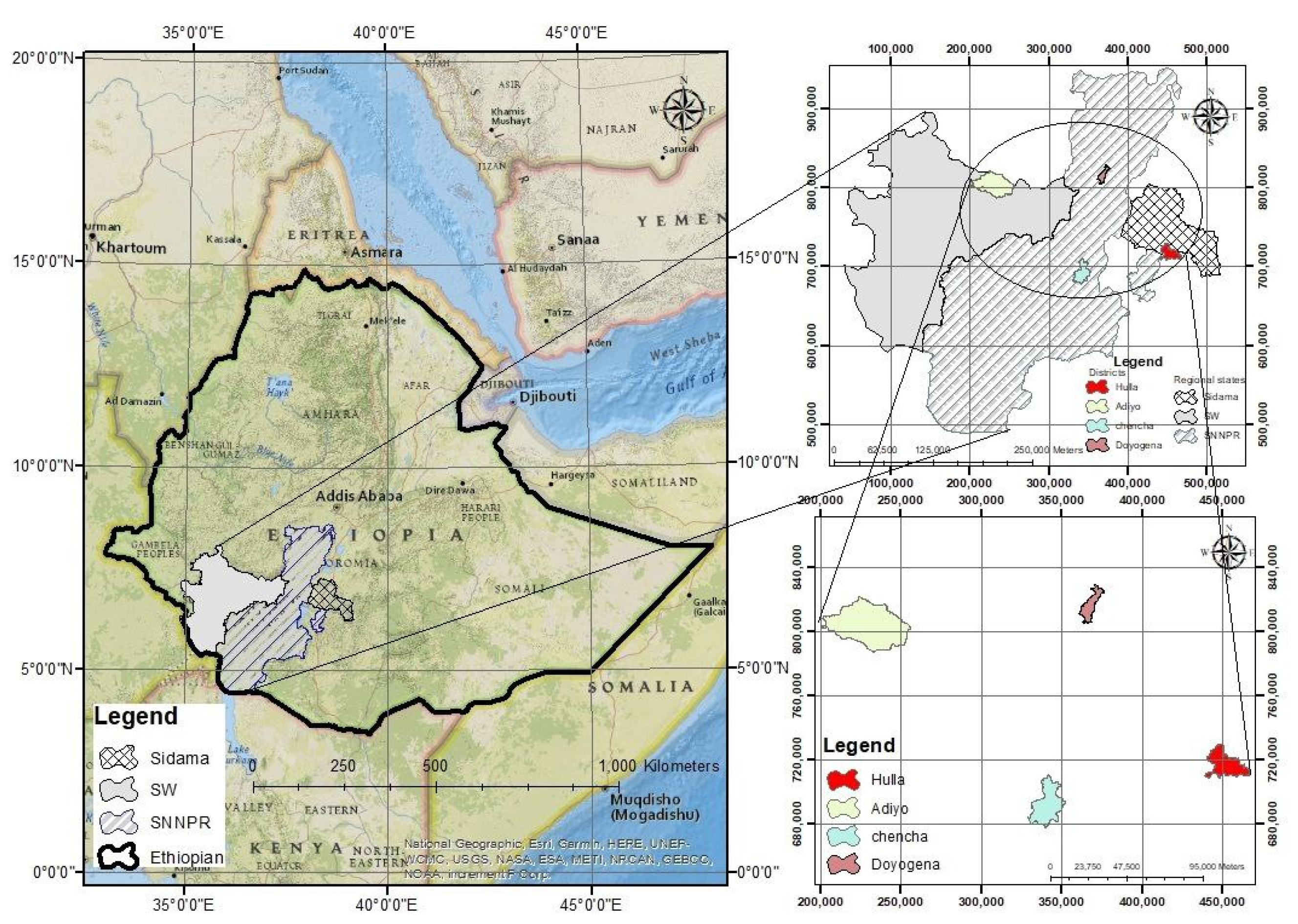
3.1. Description of Study Area
3.2. Experimental Materials
3.3. Experimental Design and Management
3.4. Data Analysis
3.4.1. AMMI Analysis
3.4.2. AMMI Stability Value (ASV) Analysis
3.4.3. Genotype Selection Index (GSI) Analysis
3.4.4. Gene Gene Environment Biplot
4. Conclusions
Author Contributions
Funding
Institutional Review Board Statement
Data Availability Statement
Acknowledgments
Conflicts of Interest
References
- Fekede, F.; Gezahegn, K. Feed Availability, Conservation Practices and Utilization in Selected Milk-Shed Areas in the Central Highlands of Ethiopia. Ethiop. J. Anim. Prod. 2018, 18, 1–9. [Google Scholar]
- Arunachalam, A.; Misra, A.K. DARE-ICAR Global Reach; Indian Council of Agricultural Research: New Delhi, India, 2020; pp. 26–34. [Google Scholar]
- Seré, C.; Ayantunde, A.; Duncan, A.; Freeman, A.; Herrero, M.; Tarawali, S.A.; Wright, I. Livestock production and poverty alleviation—Challenges and opportunities in arid and semi-arid tropical rangeland based systems. In Proceedings of the Multifunctional Grasslands in a Changing World, Volume 1: XXI International Grassland Congress and VIII International Rangeland Congress, Hohhot, China, 29 June–5 July 2008; Guangdong People’s Publishing House: Guangzhou, China, 2008; pp. 19–26. [Google Scholar]
- FAO. 2011. Available online: http://faostat.fao.org (accessed on 20 June 2023).
- Sánchez-Martín, J.; Rubiales, D.; Flores, F.; Emeran, A.A.; Shtaya, M.J.Y.; Sillero, J.C.; Allagui, M.B.; Prats, E. Adaptation of oat (Avena sativa) cultivars to autumn sowings in Mediterranean environments. Field Crops Res. 2014, 156, 111–122. [Google Scholar] [CrossRef]
- Hoffman, L.A. The Oat Crop: Production and Utilization; Springer: Berlin/Heidelberg, Germany, 1995; p. 584. [Google Scholar]
- Suttie, S.G.; Reynolds, J.M. (Eds.) Fodder Oats: A World Overview (No. 33); Food & Agriculture Organization of United Nations: Rome, Italy, 2004; pp. 179–196. [Google Scholar]
- Anderson, T.; Lee, C.-R. Strong Selection Genome-Wide Enhances Fitness Trade-Offs Across Environments and Episodes of Selection. Evolution 2014, 68, 16–31. [Google Scholar] [CrossRef] [PubMed]
- Rodrigues, P.C.; Malosetti, M.; Gauch, H.G.; van Eeuwijk, F.A. A Weighted AMMI Algorithm to Study Genotype-by-Environment Interaction and QTL-by-Environment Interaction. Crop Sci. 2014, 54, 1555–1570. [Google Scholar] [CrossRef]
- Van Eeuwijk, F.A.; Bustos-Korts, D.V.; Malosetti, M. What should students in plant breeding know about the statistical aspects of genotype x Environment interactions? Crop Sci. 2016, 56, 2119–2140. [Google Scholar] [CrossRef]
- Begna, T. The role of genotype by environmental interaction in plant breeding. Int. J. Agric. Biosci. 2020, 9, 209–215. [Google Scholar]
- Eskridge, K.M. Selection of Stable Cultivars Using a Safety-First Rule. Crop Sci. 1990, 30, 369. [Google Scholar] [CrossRef]
- Doehlert, D.C.; McMullen, M.S.; Hammond, J.J. Genotypic and environmental effects on grain yield and quality of oat grown in North Dakota. Crop Sci. 2001, 41, 1066–1072. [Google Scholar] [CrossRef]
- Mult, Z.; Akay, H.; Köse, D.E. Grain yield, quality traits and grain yield stability of local oat cultivars. J. Soil Sci. Plant Nutr. 2018, 18, 269–281. [Google Scholar] [CrossRef]
- Milenković, J.; Blagojevića, M.; Đorđević, N.; Dinića, B.; Vasića, T.; Marković, J.; Petrovića, M. Determination of Green Forage and Silage Protein Degradability of Some Pea (Pisum sativum L.) + Oat (Avena sativa L.) Mixtures Grown in Serbia. J. Agric. Sci. 2016, 23, 415–422. [Google Scholar] [CrossRef]
- Yan, W.; Tinker, N.A. Biplot analysis of multi-environment trial data: Principles and applications. Can. J. Plant Sci. 2006, 86, 623–645. [Google Scholar] [CrossRef]
- Zobel, R.W.; Wright, M.J.; Gauch, H.G. Statistical Analysis of a Yield Trial. Agron. J. 1988, 80, 388–393. [Google Scholar] [CrossRef]
- Gauch, H.G.; Zobel, R.W. AMMI Analysis of Yield Trials. In Genotype-by-Environment Interaction; Kang, M.S., Gauch, H.G., Eds.; Taylor and Francis: Abingdon, UK, 1996; pp. 85–122. [Google Scholar]
- Yan, W.; Kang, M.S.; Woods BMa, S.; Cornelius, P.L. GGE biplot vs. AMMI analysis of genotype-by-environment data. Crop Sci. 2007, 47, 643–655. [Google Scholar] [CrossRef]
- Samonte, S.O.P.B.; Wilson, L.T.; McClung, A.M.A.M.; Medley, J.C. Targeting cultivars onto rice growing environments using AMM and SREG GGE biplot analyses. Crop Sci. 2005, 45, 2414–2424. [Google Scholar] [CrossRef]
- Rad, M.R.N.; Kadir, M.A.; Rafii, M.Y.; Jaafar, H.Z.E.; Naghavi, M.R.; Ahmadi, F. Genotype × environment interaction by AMMI and GGE biplot analysis in three consecutive generations of wheat (Triticum aestivum) under normal and drought stress conditions. Aust. J. Crop Sci. 2013, 7, 956–961. [Google Scholar]
- Gauch, H.G. Statistical analysis of yield trials by AMMI and GGE. Crop Sci. 2006, 46, 1488–1500. [Google Scholar] [CrossRef]
- Gauch, H.G.; Piepho, H.P.; Annicchiarico, P. Statistical analysis of yield trials by AMMI and GGE: Further considerations. Crop Sci. 2008, 48, 866–889. [Google Scholar] [CrossRef]
- Yan, W.; Frégeau-Reid, J.; Pageau, D.; Martin, R. Genotype-by-environment interaction and trait associations in two genetic populations of oat. Crop Sci. 2016, 56, 1136–1145. [Google Scholar] [CrossRef]
- Hmwe, S.S.; Htun, T.M.; Win, S.; Aung, M.M.; Tan, A.M. Genotype and environment interaction on yield in cassava (Manihot esculenta). J. Agric. Res. 2018, 5, 62–66. [Google Scholar]
- Noerwijati, K.; Nasrullah; Taryono; Prajitno, D. Fresh Tuber Yield Stability Analysis of Fifteen Cassava Genotypes Across Five Environments in East Java (Indonesia) Using GGE Biplot. Energy Procedia 2014, 47, 156–165. [Google Scholar] [CrossRef]
- Adjebeng-Danquah, J.; Manu-Aduening, J.; Gracen, V.E.; Asante, I.K.; Offei, S.K. AMMI Stability Analysis and Estimation of Genetic Parameters for Growth and Yield Components in Cassava in the Forest and Guinea Savannah Ecologies of Ghana. Int. J. Agron. 2017, 2017, 8075846. [Google Scholar] [CrossRef]
- Abera, L.M.W. Stability analysis of Ethiopian maize varieties using AMMI model. Ethiop. J. Agric. Sci. 2005, 18, 173–180. [Google Scholar]
- Temesgen, N.; Chaba, A.; Mangistu, C.; Lule, G.; Geleta, N. Regression and additive main effects and multiple interactions (AMMI) in common bean (Phaseolus vulgaris L.) genotypes. Ethiop. J. Biol. Sci. 2008, 7, 45–53. [Google Scholar]
- Misra, R.C.; Das, S.; Patnaik, M.C. AMMI Model Analysis of Stability and Adaptability of Late Duration Finger Millet (Eleusine coracana) Genotypes. World Appl. Sci. J. 2009, 6, 1650–1654. [Google Scholar]
- Girma, M.N.G.; Chemeda, D.; Abeya, T.; Dagnachew, L. Genotype x Environment Interaction for Yield in Field Pea (Pisum sativum L.). East Afr. J. Sci. 2011, 5, 6–11. [Google Scholar]
- Acciaresi, C.B.; Chidichimo, H.A.; Fusé, H.O. Study of Genotype x Environment Interaction for Forage Yield in Oat (Avena sativa L.) with Joint Linear Regression Analysis and AMMI Analysis. Cereal Res. Commun. 1997, 25, 55–62. [Google Scholar] [CrossRef]
- Hopkins, A.A.; Vogel, K.P.; Moore, K.J.; Johnson, K.D.; Carlson, I.T. Genotype Effects and Genotype by Environment Interactions for Traits of Elite Switchgrass Populations. Crop. Sci. 1995, 35, 125–132. [Google Scholar] [CrossRef]
- Yan, W.; Rajcan, I. Biplot analysis of test sites and trait relations of soybean in Ontario. Crop Sci. 2002, 42, 11–20. [Google Scholar] [CrossRef]
- Yan, W.; Hunt, L.A.; Sheng, Q.; Szlavnics, Z. Cultivar evaluation and mega-environment investigation based on the GGE biplot. Crop Sci. 2000, 40, 597–605. [Google Scholar] [CrossRef]
- Akter, A.; Hasan, M.J.; Kulsum, U.; Rahman, M.; Khatun, M.; Islam, M. GGE Biplot Analysis for Yield Stability in Multi-environment Trials of Promising Hybrid Rice (Oryza sativa L.). Bangladesh Rice J. 2015, 19, 1–8. [Google Scholar] [CrossRef]
- Erdemci, I. Investigation of genotype x environment interaction in chickpea genotypes using AMMI and GGE biplot analysis. Turk. J. Field Crop 2018, 23, 20–26. [Google Scholar] [CrossRef]
- Purchase, J. Parametric Analysis to Describe Genotype by Environment Interaction and Yield Stability in Winter Wheat. Ph.D. Thesis, University of the Free State, Bloemfontein, South Africa, 1997; p. 83. [Google Scholar]
- Wardofa, G.A.; Mohammed, H.; Asnake, D.; Alemu, T. Genotype X Environment Interaction and Yield Stability of Bread Wheat Genotypes in central Ethiopia. J. Plant Breed. Genet. 2019, 7, 87–94. [Google Scholar] [CrossRef]
- Purchase, J.L.; Hatting, H.; van Deventer, C.S. Genotype x environment interaction of winter wheat (Triticum aestivum L.) in South Africa: II. Stability analysis of yield performance. S. Afr. J. Plant Soil 2000, 17, 101–107. [Google Scholar] [CrossRef]
- Mohammadi, R.; Abdulahi, A.; Haghparast, R.; Armion, M. Interpreting genotype x environment interactions for durum wheat grain yields using nonparametric methods. Euphytica 2007, 157, 239–251. [Google Scholar] [CrossRef]
- Tadese, D. Stability Analysis Using GGE Biplot and Linear Mixed Model Analysis by R Using. 2019. Available online: http://hdl.handle.net/123456789/3148 (accessed on 20 June 2023).
- Farshadfar, E. Incorporation of AMMI stability value and grain yield in a single non-parametric index (GSI) in bread wheat. Pak. J. Biol. Sci. 2008, 11, 1791–1796. [Google Scholar] [CrossRef]
- Sholihin. GGE and AMMI biplot for interpreting interaction of genotype X environments of cassava promising genotypes. AIP Conf. Proc. 2021, 2331, 2–10. [Google Scholar] [CrossRef]
- Agyeman, A.; Parkes, E.; Peprah, B.B. AMMI and GGE biplot analysis of root yield performance of cassava genotypes in the forest and coastal ecologies. Int. J. Agric. Policy Res. 2015, 3, 222–232. [Google Scholar]
- Akinwale, M.G.; Akinyele, B.O.; Odiyi, A.C.; Dixon, A.G.O. Genotype X Environment Interaction and Yield Performance of 43 Improved Cassava (Manihot esculenta Crantz) Genotypes at Three Agro-climatic Zones in Nigeria. Br. Biotechnol. J. 2011, 1, 68–84. [Google Scholar] [CrossRef]
- Daemo, B.B.; Yohannes, D.B.; Beyene, T.M.; Abtew, W.G. AMMI and GGE Biplot Analyses for Mega Environment Identification and Selection of Some High-Yielding Cassava Genotypes for Multiple Environments. Int. J. Agron. 2023, 2023, 6759698. [Google Scholar] [CrossRef]
- Taner S, İ.; Kaya, Y.; Palta, Ç.; Taner, S. Additive Main Effects and Multiplicative Interactions Analysis of Yield Performances in Bread Wheat Genotypes across Environments Additive Main Effects and Multiplicative Interactions Analysis of Yield Performances in Bread Wheat Genotypes across Environm. Turk. J. Agric. For. 2002, 26, 275–279. [Google Scholar]
- Baraki, F.; Gebregergis, Z.; Belay, Y.; Berhe, M.; Zibelo, H. Genotype x environment interaction and yield stability analysis of mung bean (Vigna radiata (L.) Wilczek) genotypes in Northern Ethiopia. Cogent Food Agric. 2020, 6, 1729581. [Google Scholar] [CrossRef]
- Farshadfar, E.; Mohammadi, R.; Aghaee, M.; Vaisi, Z. GGE biplot analysis of genotype x environment interaction in wheat-barley disomic addition lines. Aust. J. Crop Sci. 2012, 6, 1047–1079. [Google Scholar]
- Nimlamai, T.; Banterng, P.; Jogloy, S.; Vorasoot, N. Starch accumulation of cassava genotypes grown in paddy fields during off-season. Sabrao J. Breed. Genet. 2020, 52, 109–126. [Google Scholar]
- Mitroviã, B.; Treski, S.; Stojakoviã, M.; Ivanoviã, M.; Bekavac, G. Evaluation of Experimental Maize Hybrids Tested in Multi-Location Trials Using AMMI and GGE Biplot Analyses. Turk. J. Field Crop 2012, 17, 35–40. [Google Scholar]
- Kaya, Y.; Akçura, M.; Taner, S. GGE-Biplot analysis of multi-environment yield trials in bread wheat. Turk. J. Agric. For. 2006, 30, 325–337. [Google Scholar]
- Mohamed, N.; Said, A.; Amein, K. Additive main effects and multiplicative interaction (AMMI) and GGE-biplot analysis of genotype x environment interactions for grain yield in bread wheat (Triticum aestivum L.). Afr. J. Agric. Res. 2013, 8, 5197–5203. [Google Scholar] [CrossRef]
- Chipeta, M.M.; Melis, R.; Shanahan, P.; Sibiya, J.; Benesi IR, M. Genotype x environment interaction and stability analysis of cassava genotypes at different harvest times. J. Anim. Plant Sci. 2017, 27, 901–919. [Google Scholar]
- Jalata, Z. GGE-biplot Analysis of Multi-environment yield trials of barley genotypes in Southeastern Ethiopia Highlands. Int. J. Plant Breed. Genet. 2011, 5, 59–75. [Google Scholar] [CrossRef]
- Voltas, J.; van Eeuwijk, F.; Igartua, E.; Garcia del Moral, L.F.; Molina-Cano, J.L.; Romagosa, I. Genotype by environment interaction and adaptation in barley breeding: Basic concepts and methods of analysis. Barley Sci. Recent Adv. Mol. Biol. Agron. Yield Qual. 2002, 205–241. [Google Scholar]
- Neisse, A.C.; Kirch, J.L.; Hongyu, K. AMMI and GGE Biplot for genotype x environment interaction: A medoid–based hierarchical cluster analysis approach for high–dimensional data. Biometrical Lett. 2018, 55, 97–121. [Google Scholar] [CrossRef]
- Yan, W.; Hunt, L.A. Interpretation The GE Interacaction for Winter Wheat Yield in Ontario. Crop Sci. 2002, 41, 19–25. [Google Scholar] [CrossRef]
- Abebe, S.M.; Gurmu, F.; Mekonen, S. Root Yield Stability Analysis of White-Fleshed Sweet Potato Genotypes in Ethiopia. Adv. Crop Sci. Technol. 2019, 7, 429. [Google Scholar] [CrossRef]
- Gauch, H.G., Jr. Statistical Analysis of Regional Yield Trials: AMMI Analysis of Factorial Designs; Elsevier Science Publishers: Amsterdam, The Netherlands, 1992. [Google Scholar]
- Miranda, G.V.; de Souza, L.V.; Guimarães, M.; Namorato, H.; Oliveira, L.R.; Soares, M.O. Multivariate analyses of genotype x environment interaction of popcorn. Pesqui. Agropecuária Bras. 2009, 44, 45–50. [Google Scholar] [CrossRef]
- Payne, A.D.; Baird, R.W.; Cherry, D.B.; Gilmour, M.; Harding, A.R.; Lane, S.A.; Morgan, P.W.; Murray, G.W.; Soutar, D.A.; Thompson, D.M.; et al. GenStat Release Reference Manual; Part 2. Directives; VSN International: Hertfordshire, UK, 2002. [Google Scholar]
- Hugh, G.; Gauch, J. Model Selection and Validation for Yield Trials with Interaction. Biometrics 1988, 4, 705–715. [Google Scholar]


| Source | D.F. | S.S. | M.S. | (%) SS Explained |
|---|---|---|---|---|
| Total | 263 | 3052.9 | 11.61 | |
| Treatments | 43 | 1052.3 | 24.47 *** | |
| Genotypes | 10 | 367.6 | 36.76 *** | 34.94 |
| Environments | 3 | 164.2 | 54.72 ** | 15.60 |
| Block | 8 | 92.7 | 11.59 | |
| Interactions | 30 | 520.5 | 17.35 ** | 49.46 |
| IPCA 1 | 12 | 381.8 | 31.81 *** | 73.35 |
| IPCA 2 | 10 | 77.9 | 7.79 | 14.97 |
| Residuals | −6 | 0 | 0 | |
| Error | 212 | 1907.9 | 9 |
| Genotypes | Environments | Genotypic Mean | Rank | ||||
|---|---|---|---|---|---|---|---|
| Code | Name | Chencha | Adiyo | Doyogena | Hulla | ||
| G1 | ILRI_5431A | 8.30 | 10.26 | 11.11 | 8.85 | 9.63 | 3 |
| G2 | ILRI_5444A | 7.08 | 11.38 | 11.55 | 7.02 | 9.26 | 6 |
| G3 | ILRI_5490A | 9.47 | 7.88 | 10.93 | 6.72 | 8.75 | 10 |
| G4 | ILRI_5499A | 8.89 | 9.75 | 10.67 | 7.82 | 9.29 | 5 |
| G5 | ILRI_5526A | 11.51 | 11.67 | 11.65 | 11.75 | 11.65 | 2 |
| G6 | ILRI_5527A | 12.48 | 12.65 | 12.77 | 12.17 | 12.52 | 1 |
| G7 | ILRI_15152A | 10.47 | 11.11 | 3.01 | 9.99 | 8.65 | 11 |
| G8 | ILRI_15153A | 8.99 | 11.38 | 8.60 | 7.72 | 9.17 | 7 |
| G9 | ILRI_16101A | 8.75 | 9.88 | 9.69 | 7.82 | 9.03 | 9 |
| G10 | SRCPX80AB2291 | 8.23 | 10.09 | 10.31 | 7.53 | 9.04 | 8 |
| G11 | SRCPX80AB2806 | 10.69 | 11.36 | 9.52 | 11.36 | 9.43 | 4 |
| Environmental Mean | 9.53(3) | 10.67(1) | 9.98(2) | 8.50(4) | 9.67 | ||
| LSD (5%) | 2.81 | 2.88 | 3.55 | 3.12 | |||
| CV (%) | 15.46 | 14.93 | 18.75 | 21.72 | |||
| F value | ** | *** | * | ** | |||
| Genotypes | BYDM | RY | GSI | ASV | RASV | IPCA1 | IPCA2 |
|---|---|---|---|---|---|---|---|
| G1 | 9.63 | 3 | 11 | 0.937532498 | 8 | −0.46271 | 0.32331 |
| G2 | 9.26 | 6 | 16 | 1.793726372 | 10 | −0.88151 | −0.73616 |
| G3 | 8.75 | 10 | 19 | 1.45376979 | 9 | −0.7156 | 0.56232 |
| G4 | 9.29 | 5 | 12 | 0.86520405 | 7 | −0.42998 | 0.16699 |
| G5 | 11.65 | 2 | 6 | 0.492768176 | 4 | 0.18251 | 0.80585 |
| G6 | 12.52 | 1 | 3 | 0.290958358 | 2 | 0.06914 | 0.62493 |
| G7 | 8.65 | 11 | 22 | 4.900847781 | 11 | 2.4432 | −0.01007 |
| G8 | 9.17 | 7 | 12 | 0.679687821 | 5 | 0.314 | −0.62413 |
| G9 | 9.03 | 9 | 10 | 0.277265348 | 1 | −0.13761 | 0.06356 |
| G10 | 9.04 | 8 | 14 | 1.982438484 | 6 | −0.40402 | −0.09492 |
| G11 | 9.43 | 4 | 7 | 1.08732656 | 3 | 0.02258 | −1.08168 |
| Location | Altitude (m.a.s.l) | Annual Av RF (mm) | Soil Type | Max T° | Min T° | pH |
|---|---|---|---|---|---|---|
| Adiyo | 2573 | 2042.43 | Clay loam | 23.11 | 14.07 | 5.2 |
| Doyogena | 2535 | 1823.13 | Clay loam | 24.49 | 13.98 | 6.5 |
| Hulla | 2959 | 1255.39 | Clay silt | 25.15 | 13.99 | 5.0 |
| Chencha | 2985 | 1857.95 | Nitosols | 26.28 | 15.57 | 4.5 |
| Genotype Name | Genotype Code | Status |
|---|---|---|
| ILRI_5431A | G1 | Promising |
| ILRI_5444A | G2 | Promising |
| ILRI_5490A | G3 | Promising |
| ILRI_5499A | G4 | Promising |
| ILRI_5526A | G5 | Promising |
| ILRI_5527A | G6 | Promising |
| ILRI_15152A | G7 | Promising |
| ILRI_15153A | G8 | Promising |
| ILRI_16101A | G9 | Promising |
| SRCPX80AB2291 | G10 | Released |
| SRCPX80AB2806 | G11 | Released |
Disclaimer/Publisher’s Note: The statements, opinions and data contained in all publications are solely those of the individual author(s) and contributor(s) and not of MDPI and/or the editor(s). MDPI and/or the editor(s) disclaim responsibility for any injury to people or property resulting from any ideas, methods, instructions or products referred to in the content. |
© 2023 by the authors. Licensee MDPI, Basel, Switzerland. This article is an open access article distributed under the terms and conditions of the Creative Commons Attribution (CC BY) license (https://creativecommons.org/licenses/by/4.0/).
Share and Cite
Wodebo, K.Y.; Tolemariam, T.; Demeke, S.; Garedew, W.; Tesfaye, T.; Zeleke, M.; Gemiyu, D.; Bedeke, W.; Wamatu, J.; Sharma, M. AMMI and GGE Biplot Analyses for Mega-Environment Identification and Selection of Some High-Yielding Oat (Avena sativa L.) Genotypes for Multiple Environments. Plants 2023, 12, 3064. https://doi.org/10.3390/plants12173064
Wodebo KY, Tolemariam T, Demeke S, Garedew W, Tesfaye T, Zeleke M, Gemiyu D, Bedeke W, Wamatu J, Sharma M. AMMI and GGE Biplot Analyses for Mega-Environment Identification and Selection of Some High-Yielding Oat (Avena sativa L.) Genotypes for Multiple Environments. Plants. 2023; 12(17):3064. https://doi.org/10.3390/plants12173064
Chicago/Turabian StyleWodebo, Kibreab Yosefe, Taye Tolemariam, Solomon Demeke, Weyessa Garedew, Tessema Tesfaye, Muluken Zeleke, Deribe Gemiyu, Worku Bedeke, Jane Wamatu, and Mamta Sharma. 2023. "AMMI and GGE Biplot Analyses for Mega-Environment Identification and Selection of Some High-Yielding Oat (Avena sativa L.) Genotypes for Multiple Environments" Plants 12, no. 17: 3064. https://doi.org/10.3390/plants12173064
APA StyleWodebo, K. Y., Tolemariam, T., Demeke, S., Garedew, W., Tesfaye, T., Zeleke, M., Gemiyu, D., Bedeke, W., Wamatu, J., & Sharma, M. (2023). AMMI and GGE Biplot Analyses for Mega-Environment Identification and Selection of Some High-Yielding Oat (Avena sativa L.) Genotypes for Multiple Environments. Plants, 12(17), 3064. https://doi.org/10.3390/plants12173064