Pollen Grain Classification Based on Ensemble Transfer Learning on the Cretan Pollen Dataset

 ,
,  ,
,  ,
,  ,
,  and
and 
Abstract
:1. Introduction
2. Materials and Methods
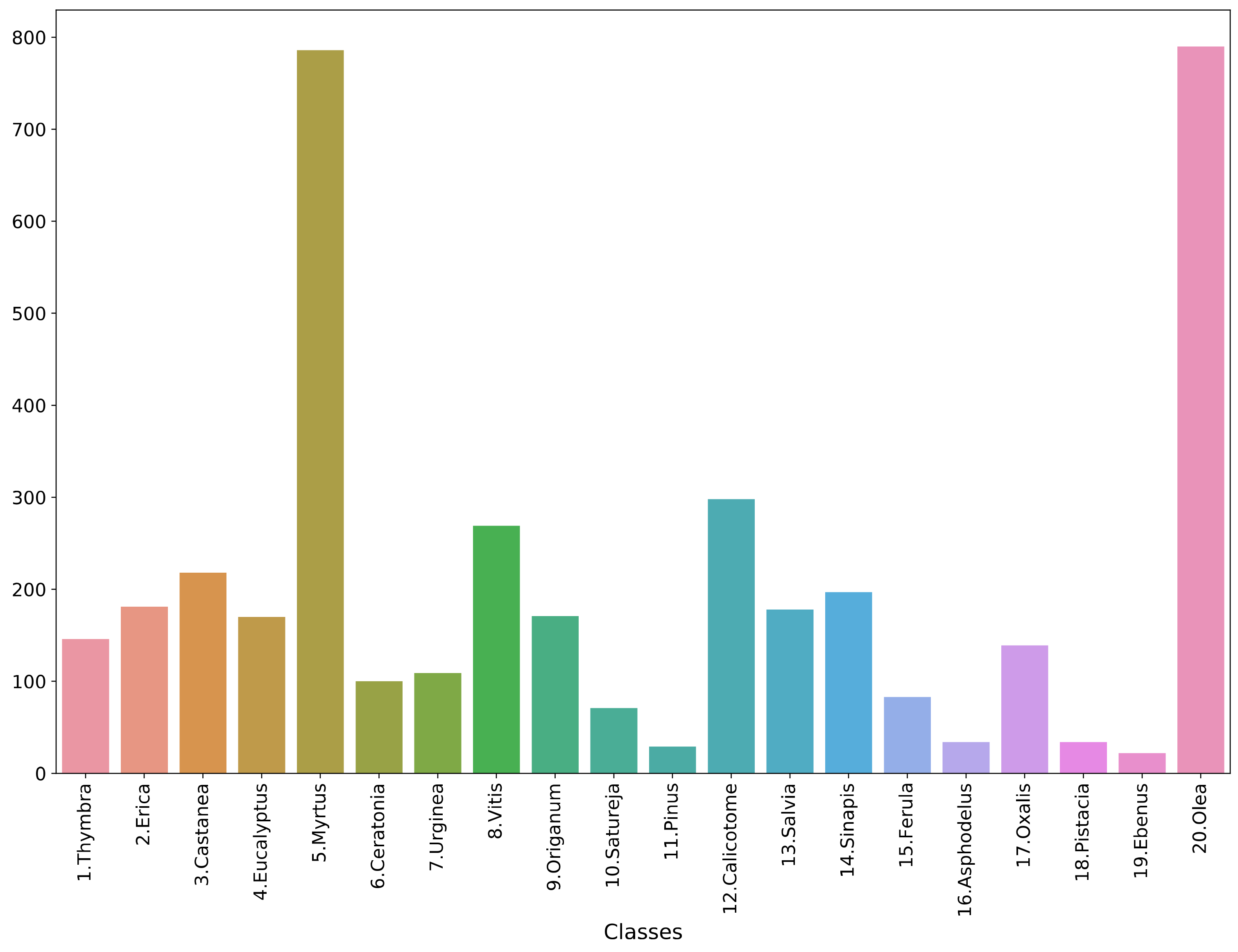
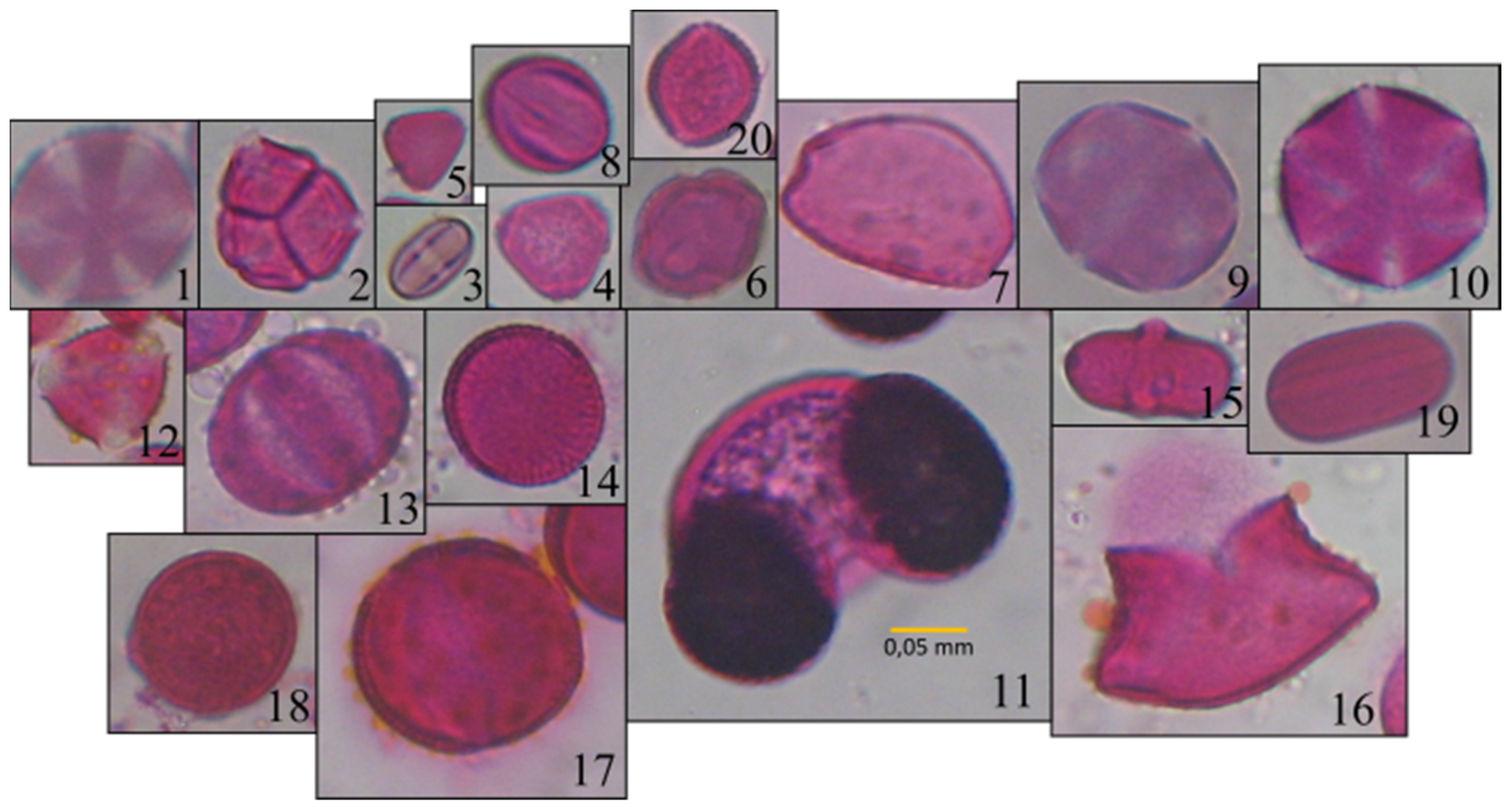
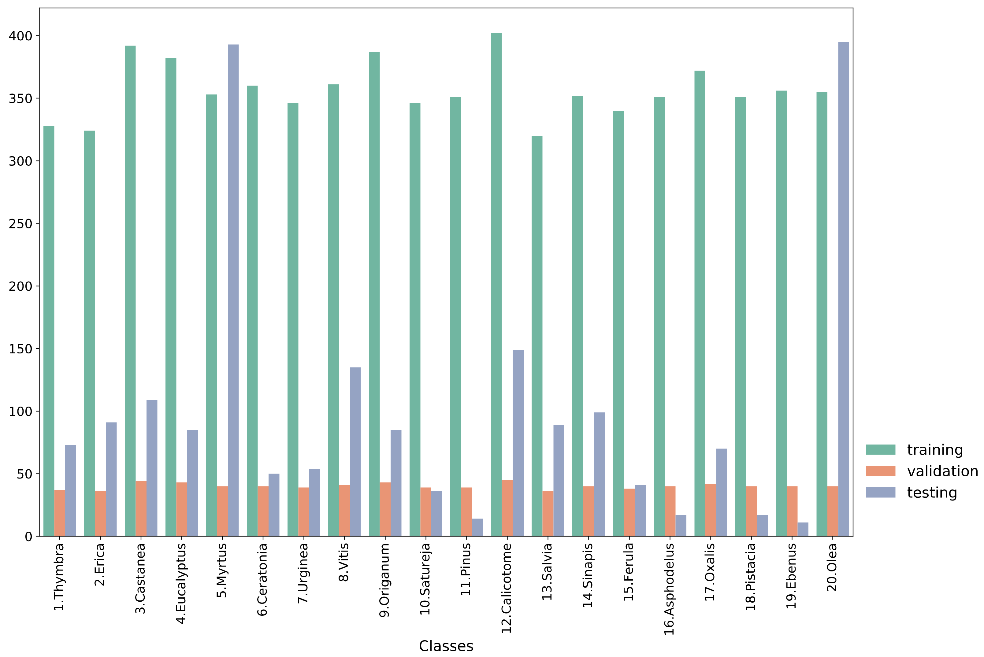
2.1. Data
2.2. Base Models
2.3. Ensemble Techniques
3. Results
3.1. Performance Metrics
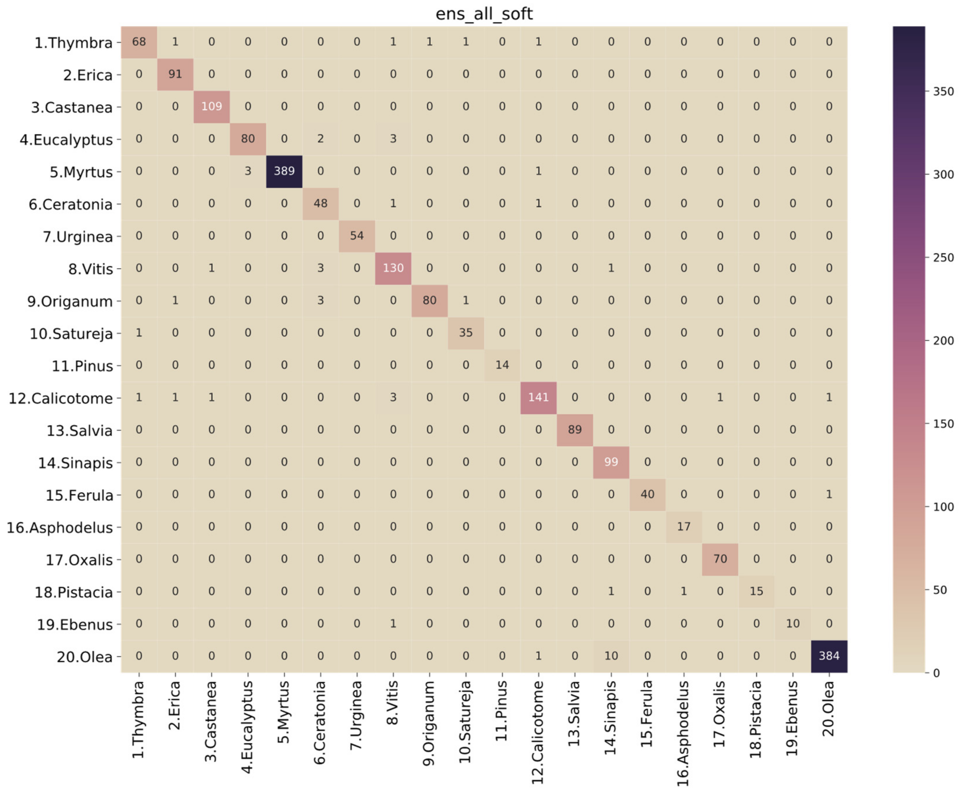
3.2. Performance Analysis of the Models
4. Discussion
4.1. Comparison to Other Studies
4.2. Performance on Honey Data
5. Conclusions
Supplementary Materials
Author Contributions
Funding
Institutional Review Board Statement
Informed Consent Statement
Data Availability Statement
Conflicts of Interest
References
- Ilia, G.; Simulescu, V.; Merghes, P.; Varan, N. The health benefits of honey as an energy source with antioxidant, antibacterial and antiseptic effects. Sci. Sports 2021, 36, 272.e1–272.e10. [Google Scholar] [CrossRef]
- Majtan, J.; Bucekova, M.; Kafantaris, I.; Szweda, P.; Hammer, K.; Mossialos, D. Honey antibacterial activity: A neglected aspect of honey quality assurance as functional food. Trends Food Sci. Technol. 2021, 118, 870–886. [Google Scholar] [CrossRef]
- Esteva, A.; Chou, K.; Yeung, S.; Naik, N.; Madani, A.; Mottaghi, A.; Liu, Y.; Topol, E.; Dean, J.; Socher, R. Deep learning-enabled medical computer vision. NPJ Digit. Med. 2021, 4, 5. [Google Scholar] [CrossRef] [PubMed]
- Santos, L.; Santos, F.N.; Oliveira, P.M.; Shinde, P. Deep learning applications in agriculture: A short review. In Iberian Robotics Conference; Springer: Berlin/Heidelberg, Germany, 2019; pp. 139–151. [Google Scholar]
- Deng, J.; Dong, W.; Socher, R.; Li, L.-J.; Li, K.; Fei-Fei, L. ImageNet: A large-scale hierarchical image database. In Proceedings of the 2009 IEEE Conference on Computer Vision and Pattern Recognition, Miami, FL, USA, 20–25 June 2009; pp. 248–255. [Google Scholar]
- Tsiknakis, N.; Savvidaki, E.; Kafetzopoulos, S.; Manikis, G.; Vidakis, N.; Marias, K.; Alissandrakis, E. Cretan Pollen Dataset v1 (CPD-1). E. Cretan Pollen Dataset 2021, v1, 1. [Google Scholar] [CrossRef]
- Astolfi, G.; Gonçalves, A.B.; Menezes, G.V.; Borges, F.S.B.; Astolfi, A.C.M.N.; Matsubara, E.T.; Alvarez, M.; Pistori, H. POLLEN73S: An image dataset for pollen grains classification. Ecol. Inform. 2020, 60, 101165. [Google Scholar] [CrossRef]
- Gonçalves, A.B.; Souza, J.S.; Da Silva, G.G.; Cereda, M.P.; Pott, A.; Naka, M.H.; Pistori, H. Feature Extraction and Machine Learning for the Classification of Brazilian Savannah Pollen Grains. PLoS ONE 2016, 11, e0157044. [Google Scholar] [CrossRef] [PubMed] [Green Version]
- Battiato, S.; Ortis, A.; Trenta, F.; Ascari, L.; Politi, M.; Siniscalco, C. POLLEN13K: A Large Scale Microscope Pollen Grain Image Dataset. In Proceedings of the 2020 IEEE International Conference on Image Processing (ICIP), Abu Dhabi, United Arab Emirates, 25–28 October 2020; IEEE: Piscataway, NJ, USA, 2020; pp. 2456–2460. [Google Scholar]
- Goodfellow, I.; Bengio, Y.; Courville, A. Deep Learning; MIT Press: Cambridge, MA, USA, 2016. [Google Scholar]
- Szegedy, C.; Vanhoucke, V.; Ioffe, S.; Shlens, J.; Wojna, Z. Rethinking the Inception Architecture for Computer Vision. In Proceedings of the IEEE Conference on Computer Vision and Pattern Recognition (CVPR), Las Vegas, NV, USA, 27–30 June 2016; pp. 2818–2826. [Google Scholar] [CrossRef] [Green Version]
- Chollet, F. Xception: Deep learning with depthwise separable convolutions. In Proceedings of the 2017 IEEE Conference on Computer Vision and Pattern Recognition (CVPR), Honolulu, HI, USA, 21–26 July 2017; pp. 1800–1807. [Google Scholar]
- He, K.; Zhang, X.; Ren, S.; Sun, J. Deep residual learning for image recognition. In Proceedings of the 2016 IEEE Conference on Computer Vision and Pattern Recognition (CVPR), Las Vegas, NV, USA, 27–30 June 2016; pp. 770–778. [Google Scholar]
- Szegedy, C.; Ioffe, S.; Vanhoucke, V.; Alemi, A.A. Inception-v4, Inception-ResNet and the Impact of Residual Connections on Learning; AAAI Press: Palo Alto, CA, USA, 2017; pp. 4278–4284. [Google Scholar]
- Tsiknakis, N.; Savvidaki, E.; Kafetzopoulos, S.; Manikis, G.; Vidakis, N.; Marias, K.; Alissandrakis, E. Segmenting 20 Types of Pollen Grains for the Cretan Pollen Dataset v1 (CPD-1). Appl. Sci. 2021, 11, 6657. [Google Scholar] [CrossRef]
- Kingma, D.P.; Ba, J. Adam: A method for stochastic optimization. In Proceedings of the International Conference Learn, Represent, (ICLR), San Diego, CA, USA, 5–8 May 2015. [Google Scholar]
- Official Government Gazette B-239/23-2-2005 Annex II Article 67 of Greek Food Code 2005, Greek Ministry of Agriculture. Available online: http://www.et.gr/index.php/anazitisi-fek (accessed on 28 March 2022).
- Manikis, G.C.; Marias, K.; Alissandrakis, E.; Perrotto, L.; Savvidaki, E.; Vidakis, N. Pollen Grain Classification using Geometrical and Textural Features. In Proceedings of the 2019 IEEE International Conference on Imaging Systems and Techniques (IST), Abu Dhabi, United Arab Emirates, 9–10 December 2019; IEEE: Piscataway, NJ, USA, 2019; pp. 1–6. [Google Scholar]
- Battiato, S.; Ortis, A.; Trenta, F.; Ascari, L.; Politi, M.; Siniscalco, C. Detection and Classification of Pollen Grain Microscope Images. In Proceedings of the 2020 IEEE/CVF Conference on Computer Vision and Pattern Recognition Workshops (CVPRW), Seattle, WA, USA, 14–19 June 2020; pp. 4220–4227. [Google Scholar]
- Sevillano, V.; Aznarte, J.L. Improving classification of pollen grain images of the POLEN23E dataset through three different applications of deep learning convolutional neural networks. PLoS ONE 2018, 13, e0201807. [Google Scholar] [CrossRef] [PubMed] [Green Version]
- Louveaux, J.; Maurizio, A.; Vorwohl, G. Methods of Melissopalynology. BEE World 1978, 59, 139–157. [Google Scholar] [CrossRef]


| Augmentation Method | Hyperparameters | Probability |
|---|---|---|
| Gaussian Blurring | Sigma [0, 0.3] | 30% |
| Linear Contrast Adjustment | Alpha [0.75, 1.25] | 30% |
| Brightness Multiplication | Multiplication factor [0.7, 1.3] | 30% |
| Rotation | Degrees [−180, 180] | 100% |
| Translation in x Plane | Translation percentage [−0.2, 0.2] | 100% |
| Translation in y Plane | Translation percentage [−0.2, 0.2] | 100% |
| Vertical Flipping | - | 50% |
| Horizontal Flipping | - | 50% |
| Input Size | Output Size | Activation Function | |
|---|---|---|---|
| Global Average Pooling 2D | - | - | - |
| Dense Layer | - | 1024 | ReLU |
| Droput of 50% | 1024 | 1024 | - |
| Dense Layer | 1024 | 512 | ReLU |
| Droput of 50% | 512 | 512 | - |
| Dense Layer | 512 | 256 | ReLU |
| Droput of 50% | 256 | 256 | - |
| Dense Layer | 256 | 128 | ReLU |
| Droput of 50% | 1024 | 1024 | - |
| Dense Layer | 128 | 20 | Softmax |
| Models | Prediction Probability | Prediction |
|---|---|---|
| Model 1 | [0.8, 0.2] | Class 0 |
| Model 2 | [0.55, 0.45] | Class 0 |
| Model 3 | [0.1, 0.9] | Class 1 |
| Soft Voting Ensemble | [0.8 + 0.55 + 0.1, 0.2 + 0.45 + 0.9]/3 = [0.483, 0.517] | Class 1 |
| Hard Voting Ensemble | Maximum occurrence [0,0,1] | Class 0 |
| Macro | Weighted | ||||||||
|---|---|---|---|---|---|---|---|---|---|
| ACC | Pre | Sen | F1 | AUC | Pre | Sen | F1 | AUC | |
| ens_all_hard | 0.975161 | 0.970762 | 0.966647 | 0.967991 | NA | 0.976031 | 0.975161 | 0.975231 | NA |
| ens_all_soft | 0.975161 | 0.970042 | 0.969219 | 0.968880 | 0.999542 | 0.976306 | 0.975161 | 0.975334 | 0.999533 |
| ens_ir_i_r_hard | 0.972678 | 0.969362 | 0.966809 | 0.967251 | NA | 0.973837 | 0.972678 | 0.972838 | NA |
| ens_ir_i_r_soft | 0.973671 | 0.969781 | 0.966628 | 0.967443 | 0.999437 | 0.974688 | 0.973671 | 0.973803 | 0.999338 |
| ens_ir_r_hard | 0.957278 | 0.952362 | 0.947819 | 0.947840 | NA | 0.959952 | 0.957278 | 0.957202 | NA |
| ens_ir_r_soft | 0.966716 | 0.965132 | 0.963203 | 0.962795 | 0.999358 | 0.969911 | 0.966716 | 0.967410 | 0.999204 |
| ens_i_r_hard | 0.964729 | 0.959518 | 0.956076 | 0.956596 | NA | 0.966231 | 0.964729 | 0.964742 | NA |
| ens_i_r_soft | 0.974168 | 0.967764 | 0.970974 | 0.968863 | 0.999177 | 0.975065 | 0.974168 | 0.974326 | 0.999204 |
| ens_x_ir_hard | 0.959265 | 0.958602 | 0.949879 | 0.951970 | NA | 0.962451 | 0.959265 | 0.959344 | NA |
| ens_x_ir_i_hard | 0.972181 | 0.971409 | 0.969076 | 0.969541 | NA | 0.973656 | 0.972181 | 0.972402 | NA |
| ens_x_ir_i_soft | 0.974168 | 0.971959 | 0.968699 | 0.969395 | 0.999222 | 0.975805 | 0.974168 | 0.974393 | 0.999170 |
| ens_x_ir_r_hard | 0.969697 | 0.967619 | 0.964934 | 0.965034 | NA | 0.972198 | 0.969697 | 0.970201 | NA |
| ens_x_ir_r_soft | 0.971187 | 0.968954 | 0.966567 | 0.966683 | 0.999464 | 0.973259 | 0.971187 | 0.971571 | 0.999475 |
| ens_x_ir_soft | 0.966716 | 0.963960 | 0.961913 | 0.961237 | 0.998892 | 0.970550 | 0.966716 | 0.967457 | 0.998980 |
| ens_x_i_hard | 0.965723 | 0.960852 | 0.954880 | 0.956783 | NA | 0.966856 | 0.965723 | 0.965620 | NA |
| ens_x_i_r_hard | 0.976155 | 0.969923 | 0.970366 | 0.969455 | NA | 0.977386 | 0.976155 | 0.976399 | NA |
| ens_x_i_r_soft | 0.976652 | 0.969540 | 0.971659 | 0.969963 | 0.999387 | 0.977790 | 0.976652 | 0.976889 | 0.999454 |
| ens_x_i_soft | 0.974168 | 0.967077 | 0.971752 | 0.968744 | 0.998931 | 0.975470 | 0.974168 | 0.974411 | 0.999008 |
| ens_x_r_hard | 0.967213 | 0.960367 | 0.952631 | 0.954955 | NA | 0.968760 | 0.967213 | 0.967131 | NA |
| ens_x_r_soft | 0.971684 | 0.964913 | 0.963993 | 0.963454 | 0.999097 | 0.973144 | 0.971684 | 0.971921 | 0.999184 |
| inception | 0.964729 | 0.960787 | 0.961660 | 0.960547 | 0.998633 | 0.966119 | 0.964729 | 0.964959 | 0.998587 |
| inception_resnet | 0.952310 | 0.953253 | 0.952506 | 0.950253 | 0.998199 | 0.958644 | 0.952310 | 0.953534 | 0.997607 |
| resnet | 0.958271 | 0.950490 | 0.955365 | 0.951001 | 0.998360 | 0.962226 | 0.958271 | 0.959258 | 0.998233 |
| xception | 0.961749 | 0.950759 | 0.953611 | 0.950483 | 0.998096 | 0.964355 | 0.961749 | 0.962129 | 0.998363 |
| Sensitivity | Specificity | Precision | Accuracy | F1 | AUC | |
|---|---|---|---|---|---|---|
| ens_all_hard | 0.917808 | 0.998969 | 0.971014 | 0.996026 | 0.943662 | NA |
| ens_all_soft | 0.931507 | 0.998969 | 0.971429 | 0.996523 | 0.951049 | 0.999569 |
| ens_ir_i_r_hard | 0.917808 | 0.998969 | 0.971014 | 0.996026 | 0.943662 | NA |
| ens_ir_i_r_soft | 0.931507 | 0.998969 | 0.971429 | 0.996523 | 0.951049 | 0.999364 |
| ens_ir_r_hard | 0.780822 | 1.000000 | 1.000000 | 0.992052 | 0.876923 | NA |
| ens_ir_r_soft | 0.917808 | 1.000000 | 1.000000 | 0.997019 | 0.957143 | 0.998757 |
| ens_i_r_hard | 0.835616 | 0.998969 | 0.968254 | 0.993045 | 0.897059 | NA |
| ens_i_r_soft | 0.931507 | 0.997938 | 0.944444 | 0.995529 | 0.937931 | 0.999244 |
| ens_x_ir_hard | 0.821918 | 1.000000 | 1.000000 | 0.993542 | 0.902256 | NA |
| ens_x_ir_i_hard | 0.904110 | 0.998454 | 0.956522 | 0.995032 | 0.929577 | NA |
| ens_x_ir_i_soft | 0.931507 | 0.998969 | 0.971429 | 0.996523 | 0.951049 | 0.995220 |
| ens_x_ir_r_hard | 0.917808 | 0.998969 | 0.971014 | 0.996026 | 0.943662 | NA |
| ens_x_ir_r_soft | 0.904110 | 0.999485 | 0.985075 | 0.996026 | 0.942857 | 0.998913 |
| ens_x_ir_soft | 0.904110 | 1.000000 | 1.000000 | 0.996523 | 0.949640 | 0.995629 |
| ens_x_i_hard | 0.863014 | 0.998454 | 0.954545 | 0.993542 | 0.906475 | NA |
| ens_x_i_r_hard | 0.931507 | 0.998454 | 0.957746 | 0.996026 | 0.944444 | NA |
| ens_x_i_r_soft | 0.931507 | 0.998969 | 0.971429 | 0.996523 | 0.951049 | 0.999477 |
| ens_x_i_soft | 0.945205 | 0.996907 | 0.920000 | 0.995032 | 0.932432 | 0.995523 |
| ens_x_r_hard | 0.821918 | 0.998969 | 0.967742 | 0.992548 | 0.888889 | NA |
| ens_x_r_soft | 0.904110 | 0.998969 | 0.970588 | 0.995529 | 0.936170 | 0.998687 |
| inception | 0.931507 | 0.995361 | 0.883117 | 0.993045 | 0.906667 | 0.994549 |
| inception_resnet | 0.849315 | 1.000000 | 1.000000 | 0.994536 | 0.918519 | 0.993913 |
| resnet | 0.863014 | 0.997938 | 0.940299 | 0.993045 | 0.900000 | 0.997522 |
| xception | 0.904110 | 0.996907 | 0.916667 | 0.993542 | 0.910345 | 0.995763 |
| Sensitivity | Specificity | Precision | Accuracy | F1 | AUC | |
|---|---|---|---|---|---|---|
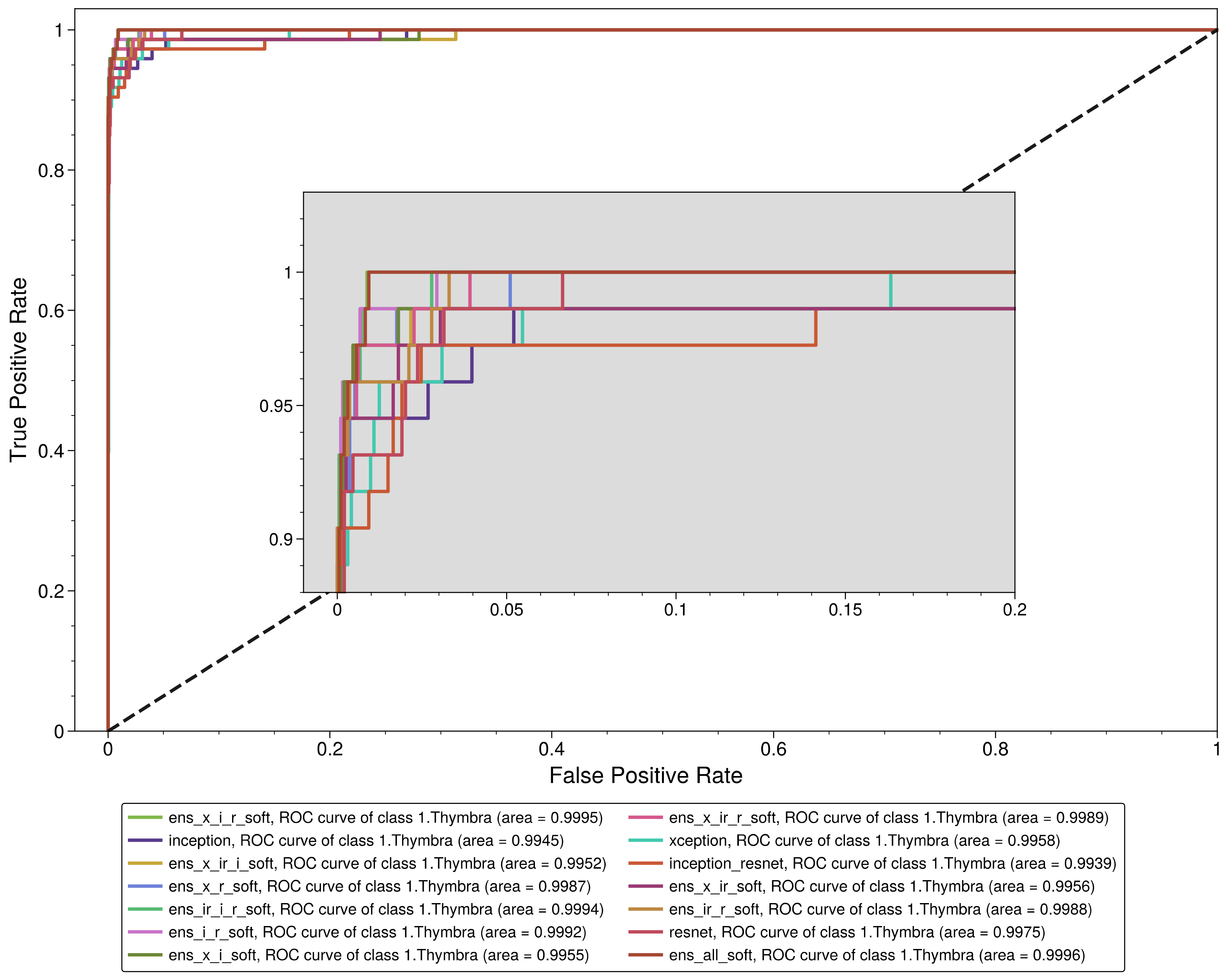
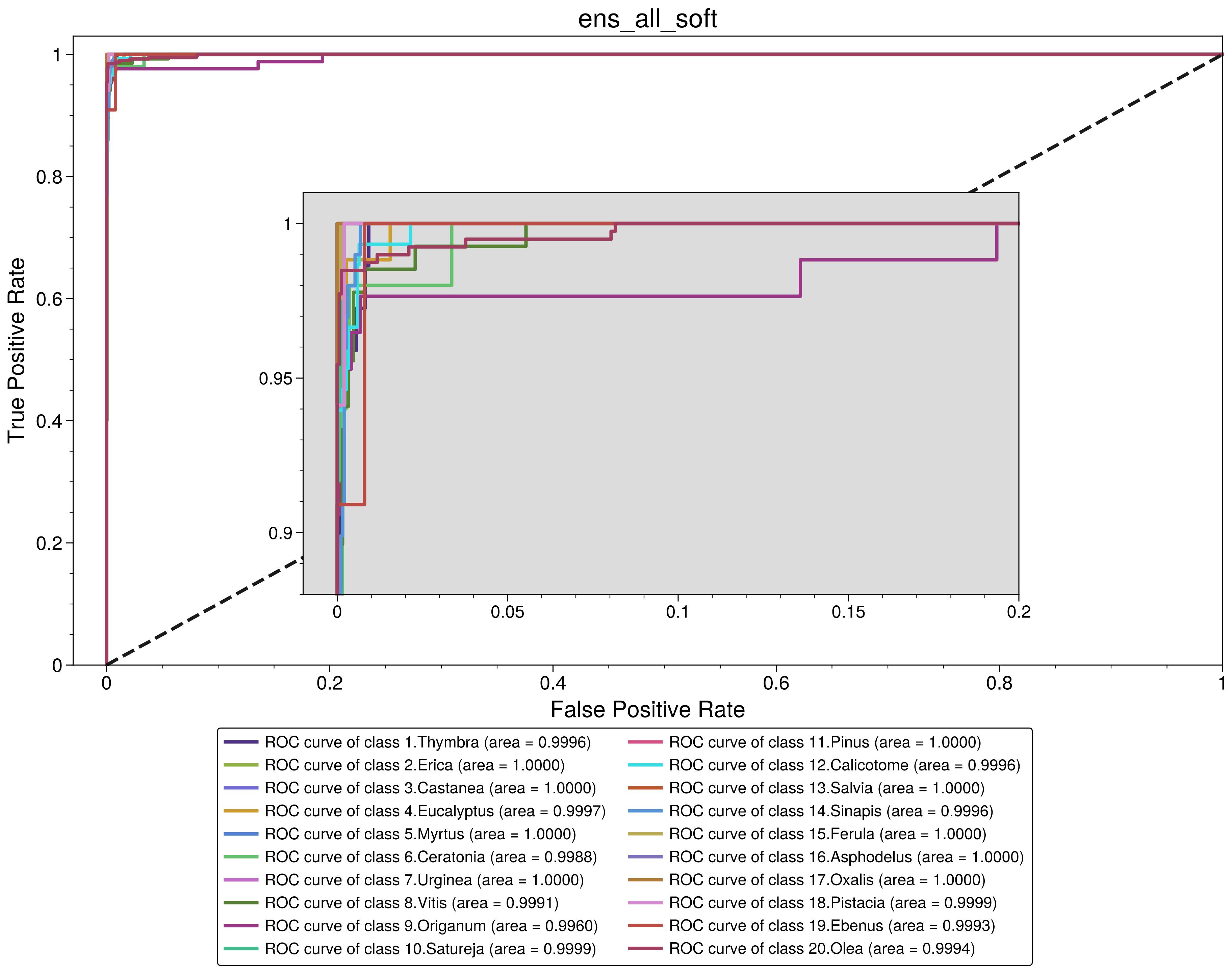
| 1. Thymbra | 0.931507 | 0.998969 | 0.971429 | 0.996523 | 0.951049 | 0.999569 |
| 2. Erica | 1.000000 | 0.998439 | 0.968085 | 0.998510 | 0.983784 | 1.000000 |
| 3. Castanea | 1.000000 | 0.998950 | 0.981982 | 0.999006 | 0.990909 | 1.000000 |
| 4. Eucalyptus | 0.941176 | 0.998444 | 0.963855 | 0.996026 | 0.952381 | 0.999713 |
| 5. Myrtus | 0.989822 | 1.000000 | 1.000000 | 0.998013 | 0.994885 | 0.999991 |
| 6. Ceratonia | 0.960000 | 0.995925 | 0.857143 | 0.995032 | 0.905660 | 0.998839 |
| 7. Urginea | 1.000000 | 1.000000 | 1.000000 | 1.000000 | 1.000000 | 1.000000 |
| 8. Vitis | 0.962963 | 0.995208 | 0.935252 | 0.993045 | 0.948905 | 0.999101 |
| 9. Origanum | 0.941176 | 0.999481 | 0.987654 | 0.997019 | 0.963855 | 0.995973 |
| 10. Satureja | 0.972222 | 0.998988 | 0.945946 | 0.998510 | 0.958904 | 0.999930 |
| 11. Pinus | 1.000000 | 1.000000 | 1.000000 | 1.000000 | 1.000000 | 1.000000 |
| 12. Calicotome | 0.946309 | 0.997854 | 0.972414 | 0.994039 | 0.959184 | 0.999622 |
| 13. Salvia | 1.000000 | 1.000000 | 1.000000 | 1.000000 | 1.000000 | 1.000000 |
| 14. Sinapis | 1.000000 | 0.993730 | 0.891892 | 0.994039 | 0.942857 | 0.999609 |
| 15. Ferula | 0.975610 | 1.000000 | 1.000000 | 0.999503 | 0.987654 | 0.999975 |
| 16. Asphodelus | 1.000000 | 0.999499 | 0.944444 | 0.999503 | 0.971429 | 1.000000 |
| 17. Oxalis | 1.000000 | 0.999485 | 0.985915 | 0.999503 | 0.992908 | 1.000000 |
| 18. Pistacia | 0.882353 | 1.000000 | 1.000000 | 0.999006 | 0.937500 | 0.999882 |
| 19. Ebenus | 0.909091 | 1.000000 | 1.000000 | 0.999503 | 0.952381 | 0.999273 |
| 20. Olea | 0.972152 | 0.998764 | 0.994819 | 0.993542 | 0.983355 | 0.999368 |
| Ref. | Method | Dataset | AUC | Sensitivity | Precision | Accuracy | F1 Score |
|---|---|---|---|---|---|---|---|
| Manikis et al. [18] | Hand-crafted Features + ML | 546 images | - | 88.16% | 88.60% | 88.24% | 87.79% |
| Battiato et al. [19] | CNN | Pollen23E 805 images | - | - | - | 89.63% | 88.97% |
| Sevillano et al. [20] | CNN + LD | Pollen23E 805 images | - | 99.64% | 94.77% | 93.22% | 96.69% |
| Astolfi et al. [7] | CNN | Pollen73S 2523 images | - | 95.7% | 95.7% | 95.8% | 96.4% |
| Our study | CNN | CPD 4034 | 0.9995 | 96.9% | 97% | 97.5% | 96.89% |
Publisher’s Note: MDPI stays neutral with regard to jurisdictional claims in published maps and institutional affiliations. |
© 2022 by the authors. Licensee MDPI, Basel, Switzerland. This article is an open access article distributed under the terms and conditions of the Creative Commons Attribution (CC BY) license (https://creativecommons.org/licenses/by/4.0/).
Share and Cite
Tsiknakis, N.; Savvidaki, E.; Manikis, G.C.; Gotsiou, P.; Remoundou, I.; Marias, K.; Alissandrakis, E.; Vidakis, N. Pollen Grain Classification Based on Ensemble Transfer Learning on the Cretan Pollen Dataset. Plants 2022, 11, 919. https://doi.org/10.3390/plants11070919
Tsiknakis N, Savvidaki E, Manikis GC, Gotsiou P, Remoundou I, Marias K, Alissandrakis E, Vidakis N. Pollen Grain Classification Based on Ensemble Transfer Learning on the Cretan Pollen Dataset. Plants. 2022; 11(7):919. https://doi.org/10.3390/plants11070919
Chicago/Turabian StyleTsiknakis, Nikos, Elisavet Savvidaki, Georgios C. Manikis, Panagiota Gotsiou, Ilektra Remoundou, Kostas Marias, Eleftherios Alissandrakis, and Nikolas Vidakis. 2022. "Pollen Grain Classification Based on Ensemble Transfer Learning on the Cretan Pollen Dataset" Plants 11, no. 7: 919. https://doi.org/10.3390/plants11070919
APA StyleTsiknakis, N., Savvidaki, E., Manikis, G. C., Gotsiou, P., Remoundou, I., Marias, K., Alissandrakis, E., & Vidakis, N. (2022). Pollen Grain Classification Based on Ensemble Transfer Learning on the Cretan Pollen Dataset. Plants, 11(7), 919. https://doi.org/10.3390/plants11070919