

Multi-Environment and Multi-Year Bayesian Analysis Approach in Coffee canephora

 , and
, and 
Abstract
1. Introduction
2. Results
3. Discussion
4. Materials and Methods
4.1. Plant Material and Field Experiments
4.2. Model Choice
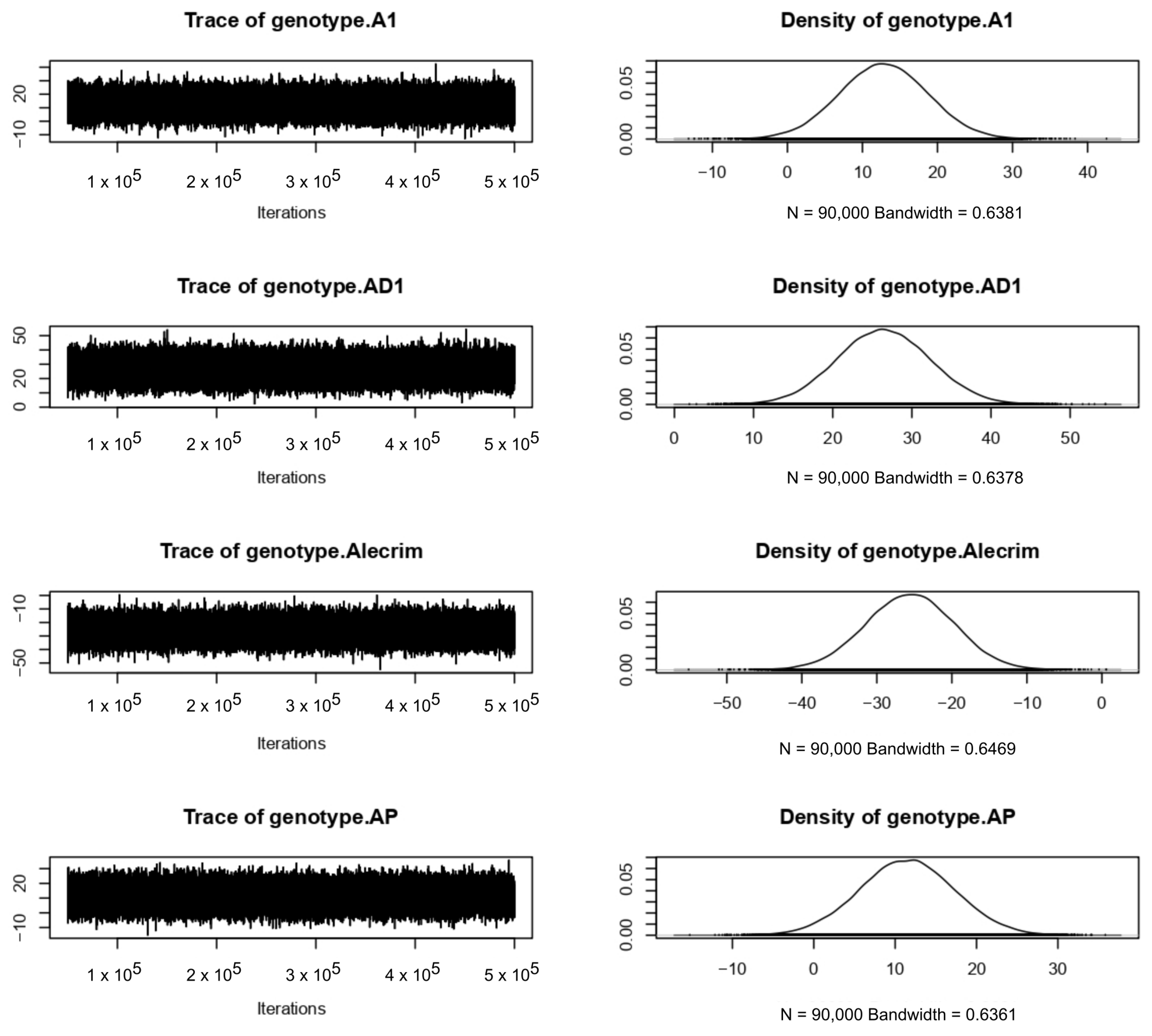
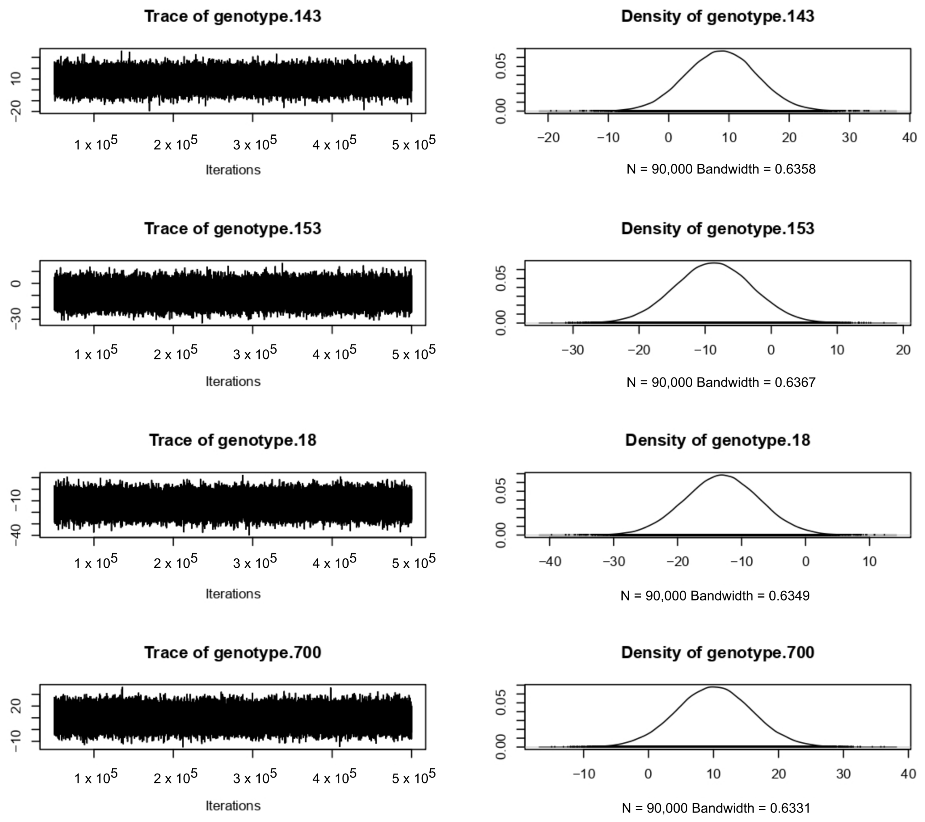
4.3. Bayesian Approach
Author Contributions
Funding
Data Availability Statement
Acknowledgments
Conflicts of Interest
Appendix A

| Heidel | ||||||
|---|---|---|---|---|---|---|
| Stationarity test | start iteration | p-value | Halfwidth test | Mean | Halfwidth | |
| genotype | passed | 1 | 0.939 | passed | 294 | 1.031 |
| environment:year | passed | 1 | 0.816 | passed | 1203 | 17.331 |
| units | passed | 1 | 0.52 | passed | 756 | 0.498 |
| Geweke | ||||||
| genotype | 0.6881 | |||||
| environment:year | 0.6316 | |||||
| units | 0.8992 | |||||
| Effective size | ||||||
| genotype | 19,982.16 | |||||
| environment:year | 18,800 | |||||
| units | 18,278.89 | |||||
| Raf Tery | ||||||
| Burn-in | Total | Lower bound | Dependence factor | |||
| genotype | 10 | 19,090 | 3746 | 5.1 | ||
| environment:year | 10 | 18,275 | 3746 | 4.88 | ||
| units | 10 | 18,600 | 3746 | 4.97 | ||


References
- USDA United States Department of Agriculture. Yld Arab and Robu Cof. 2020. Available online: https://www.usda.gov (accessed on 1 November 2022).
- CONAB. Companhia Nacional de Abastecimento—Acompanhamento Da Safra Brasileira: Acompanhamento Da Safra Brasileira de Café. Terc. Levant. 2021, 8, 1–58. [Google Scholar]
- Martins, M.Q.; Rodrigues, W.P.; Fortunato, A.S.; Leitão, A.E.; Rodrigues, A.P.; Pais, I.P.; Martins, L.D.; Silva, M.J.; Reboredo, F.H.; Partelli, F.L.; et al. Protective Response Mechanisms to Heat Stress in Interaction with High [CO2] Conditions in Coffea spp. Front. Plant Sci. 2016, 7, 947. [Google Scholar] [CrossRef] [PubMed]
- Partelli, F.L.; Vieira, H.D.; Silva, M.G.; Ramalho, J.C. Seasonal Vegetative Growth of Different Age Branches of Conilon Coffee Tree. Sem. Cien. Agr. 2010, 31, 619–626. [Google Scholar] [CrossRef]
- Ramalho, J.C.; Rodrigues, A.P.; Lidon, F.C.; Marques, L.M.C.; Leitão, A.E.; Fortunato, A.S.; Pais, I.P.; Silva, M.J.; Scotti-Campos, P.; Lopes, A.; et al. Stress Cross-Response of the Antioxidative System Promoted by Superimposed Drought and Cold Conditions in Coffea spp. PLoS ONE 2018, 13, e0198694. [Google Scholar] [CrossRef] [PubMed]
- Kath, J.; Byrareddy, V.M.; Craparo, A.; Nguyen-Huy, T.; Mushtaq, S.; Cao, L.; Bossolasco, L. Not so Robust: Robusta Coffee Production Is Highly Sensitive to Temperature. Glob. Chang. Biol. 2020, 26, 3677–3688. [Google Scholar] [CrossRef]
- Partelli, F.L.; Golynski, A.; Ferreira, A.; Martins, M.Q.; Mauri, A.L.; Ramalho, J.C.; Vieira, H.D. Andina-First Clonal Cultivar of High-Altitude Conilon Coffee. Crop Breed. Appl. Biotechnol. 2019, 19, 476–480. [Google Scholar] [CrossRef]
- Whitaker, J.; Field, J.L.; Bernacchi, C.J.; Cerri, C.E.P.; Ceulemans, R.; Davies, C.A.; DeLucia, E.H.; Donnison, I.S.; McCalmont, J.P.; Paustian, K.; et al. Consensus, Uncertainties and Challenges for Perennial Bioenergy Crops and Land Use. GCB Bioenergy 2018, 10, 150–164. [Google Scholar] [CrossRef]
- Van Eeuwijk, F.A.; Bustos-Korts, D.; Millet, E.J.; Boer, M.P.; Kruijer, W.; Thompson, A.; Malosetti, M.; Iwata, H.; Quiroz, R.; Kuppe, C. Modelling Strategies for Assessing and Increasing the Effectiveness of New Phenotyping Techniques in Plant Breeding. Plant Sci. 2019, 282, 23–39. [Google Scholar] [CrossRef]
- Labouisse, J.-P.; Cubry, P.; Austerlitz, F.; Rivallan, R.; Nguyen, H. New Insights on Spatial Genetic Structure and Diversity of Coffea canephora (Rubiaceae) in Upper Guinea Based on Old Herbaria. Plant Ecol. Evol. 2020, 153, 82–100. [Google Scholar] [CrossRef]
- Ferrão, L.F.V.; Ferrão, R.G.; Ferrão, M.A.G.; Fonseca, A.; Carbonetto, P.; Stephens, M.; Garcia, A.A.F. Accurate Genomic Prediction of Coffea canephora in Multiple Environments Using Whole-Genome Statistical Models. Heredity 2019, 122, 261–275. [Google Scholar] [CrossRef]
- Alkimim, E.R.; Caixeta, E.T.; Sousa, T.V.; da Silva, F.L.; Sakiyama, N.S.; Zambolim, L. High-Throughput Targeted Genotyping Using next-Generation Sequencing Applied in Coffea canephora Breeding. Euphytica 2018, 214, 50. [Google Scholar] [CrossRef]
- Mora, F.; Serra, N. Bayesian Estimation of Genetic Parameters for Growth, Stem Straightness, and Survival in Eucalyptus Globulus on an Andean Foothill Site. Tree Genet. Genomes 2014, 10, 711–719. [Google Scholar] [CrossRef]
- da Silva, F.A.; Viana, A.P.; Corrêa, C.C.G.; Carvalho, B.M.; de Sousa, C.M.B.; Amaral, B.D.; Ambrósio, M.; Glória, L.S. Impact of Bayesian Inference on the Selection of Psidium Guajava. Sci. Rep. 2020, 10, 1999. [Google Scholar] [CrossRef]
- Souza, A.O.; Viana, A.P.; e Silva, F.F.; Azevedo, C.F.; da Silva, F.A.; e Silva, F.H.L. Row-Col and Bayesian Approach Seeking to Improve the Predictive Capacity and Selection of Passion Fruit. Sci. Agric. 2022, 79. [Google Scholar] [CrossRef]
- Beaumont, M.A.; Rannala, B. The Bayesian Revolution in Genetics. Nat. Rev. Genet. 2004, 5, 251–261. [Google Scholar] [CrossRef]
- Silva Junqueira, V.; de Azevedo Peixoto, L.; Galvêas Laviola, B.; Lopes Bhering, L.; Mendonça, S.; Agostini Costa, T.d.S.; Antoniassi, R. Correction: Bayesian Multi-Trait Analysis Reveals a Useful Tool to Increase Oil Concentration and to Decrease Toxicity in Jatropha Curcas L. PLoS ONE 2016, 11, e0161046. [Google Scholar] [CrossRef]
- Bates, D.; Mächler, M.; Bolker, B.; Walker, S. Fitting Linear Mixed-Effects Models Using Lme4. J. Stat. Softw. 2015, 67, 48. [Google Scholar] [CrossRef]
- Matuschek, H.; Kliegl, R.; Vasishth, S.; Baayen, H.; Bates, D. Balancing Type I Error and Power in Linear Mixed Models. J. Mem. Lang. 2017, 94, 305–315. [Google Scholar] [CrossRef]
- Barr, D.J.; Levy, R.; Scheepers, C.; Tily, H.J. Random Effects Structure for Confirmatory Hypothesis Testing: Keep It Maximal. J. Mem. Lang. 2013, 68, 255–278. [Google Scholar] [CrossRef]
- Sorensen, D.; Gianola, D. Likelihood, Bayesian, and MCMC Methods in Quantitative Genetics, 1st ed.; Springer Science & Business Media: New York, NY, USA, 2007; 740p, ISBN 0387954406. [Google Scholar]
- Sandoval, V.J.C.; Silva, F.F.; Resende, M.D.V.; Macedo, L.R.; Cecon, P.R. Bayesian Random Regression for Genetic Evaluation of South American Leaf Blight in Rubber Trees. Rev. Cien. Agro. 2017, 48, 151–156. [Google Scholar] [CrossRef]
- Junqueira, V.S.; de Azevedo Peixoto, L.; Laviola, B.G.; Bhering, L.L.; Mendonça, S.; da Silveira Agostini Costa, T.; Antoniassi, R. Bayesian Multi-Trait Analysis Reveals a Useful Tool to Increase Oil Concentration and to Decrease Toxicity in Jatropha Curcas L. PLoS ONE 2016, 11, e0157038. [Google Scholar] [CrossRef]
- Carlin, B.P.; Chib, S. Bayesian Model Choice via Markov Chain Monte Carlo Methods. J. R. Stat. Soc. 1995, 57, 473–484. [Google Scholar] [CrossRef]
- Partelli, F.L.; Oliosi, G.; Dalazen, J.R.; da Silva, C.A.; Vieira, H.D.; Espindula, M.C. Proportion of Ripe Fruit Weight and Volume to Green Coffee: Differences in 43 Genotypes of Coffea canephora. Agron. J. 2021, 113, 1050–1057. [Google Scholar] [CrossRef]
- Oliosi, G.; Partelli, F.L.; da Silva, C.A.; Dubberstein, D.; Gontijo, I.; Tomaz, M.A. Seasonal Variation in Leaf Nutrient Concentration of Conilon Coffee Genotypes. J. Plant Nutr. 2021, 44, 74–85. [Google Scholar] [CrossRef]
- Sorensen, D. Developments in Statistical Analysis in Quantitative Genetics. Genetica 2009, 136, 319–332. [Google Scholar] [CrossRef]
- R Core Team. R: A Language and Environment for Statistical Computing; R Foundation for Statistical Computing: Vienna, Austria, 2020. [Google Scholar]
- Hadfield, J. MCMC Methods for Multi-Response Generalized Linear Mixed Models: The MCMCglmm R Package. J. Stat. Softw. 2010, 33, 1–22. [Google Scholar] [CrossRef]
- Cowles, M.K.; Carlin, B.P. Markov Chain Monte Carlo Convergence Diagnostics: A Comparative Review. J. Am. Stat. Assoc. 1996, 91, 883–904. [Google Scholar] [CrossRef]
- Plummer, M.; Best, N.; Cowles, K.; Vines, K. CODA: Convergence Diagnosis and Output Analysis for MCMC. R News 2006, 6, 7–11. [Google Scholar]
- Bonomo, D.Z.; Bonomo, R.; Partelli, F.L.; de Souza, J.M. Performance of Conilon Coffee Genotypes under Different Adjusted Crop Coefficients. IRRIGA 2017, 22, 236–248. [Google Scholar] [CrossRef]
- Partelli, F.L.; Giles, J.A.D.; Oliosi, G.; Covre, A.M.; Ferreira, A.; Rodrigues, V.M. Tributun: A Coffee Cultivar Developed in Partnership with Farmers. Crop Breed. Appl. Biotechnol. 2020, 20, e30002025. [Google Scholar] [CrossRef]
- Covre, A.M.; Partelli, F.L.; Bonomo, R.; Braun, H.; Ronchi, C.P. Vegetative Growth of Conilon Coffee Plants under Two Water Conditions in the Atlantic Region of Bahia State, Brazil. Acta Sci. Agron. 2016, 38, 535. [Google Scholar] [CrossRef]
- Silva, L.O.E.; Schmidt, R.; Valani, G.P.; Ferreira, A.; Ribeiro-Barros, A.I.; Partelli, F.L. Root Trait Variability in Coffea canephora Genotypes and Its Relation to Plant Height and Crop Yield. Agronomy 2020, 10, 1394. [Google Scholar] [CrossRef]


| Model | Npar | DF | Chisq | Pr (>Chisq) | Deviance | |
|---|---|---|---|---|---|---|
| 1 | Null | 2 | - | - | - | 10,579.3 |
| 2 | (1|genotype) | 3 | 1 | 91.2 | 1.2 × 10⁻²¹ | 10,488.1 |
| 3 | (1|genotype) + location | 4 | 1 | 48.8 | 2.7 × 10⁻¹² | 10,439.2 |
| 3 + 4 | (1|year) | 5 | 1 | 345.7 | 3.6 × 10−77 | 10,093.5 |
| 3 + 5 | (1|block) * | 5 | 0 | 0.0 | - | 10,438.6 |
| 3 + 6 | (1|location/year) | 6 | 1 | 557.7 | 2.5 × 10−123 | 9880.8 |
| 3 + 7 | (1|location/block) * | 6 | 0 | 0.0 | - | 10,438.6 |
| 3 + 8 | (location|year) | 7 | 1 | 559.6 | 1.0 × 10−123 | 9879.0 |
| 3 + 9 | (location|block) ** | 7 | 0 | 0.0 | - | 10,437.1 |
| 3 + 10 | (location|block) + (location|year) ** | 10 | 3 | 566.1 | 2.2 × 10−122 | 9871.0 |
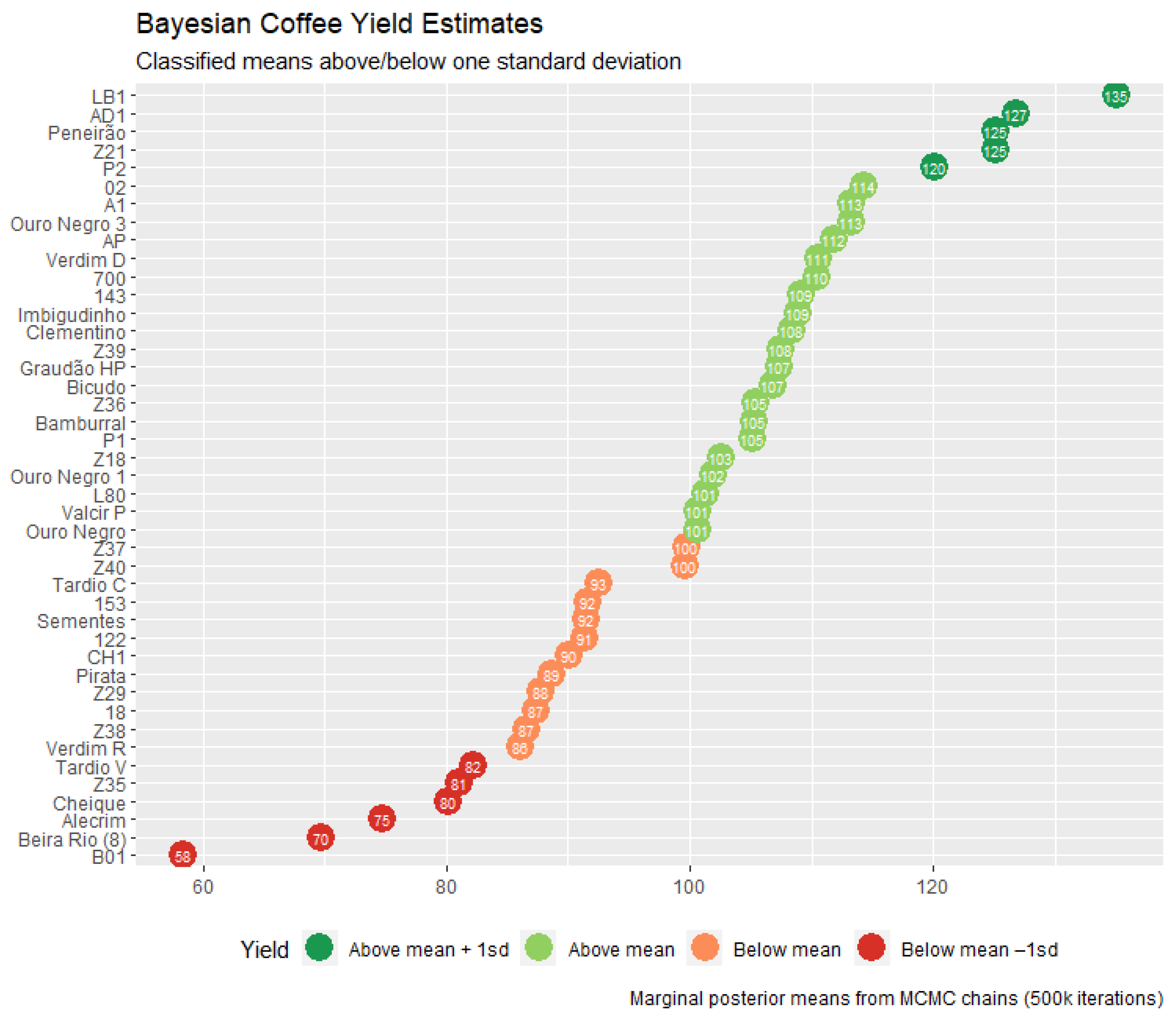
| Genotype | BLUP | HPD Interval | Genotype | BLUP | HPD Interval | ||
|---|---|---|---|---|---|---|---|
| Lower | Upper | Lower | Upper | ||||
| LB1 *,# | 34.76 | 23.41 | 46.64 | L80 # | 0.94 | −10.45 | 12.41 |
| AD1 *,# | 26.40 | 14.52 | 37.79 | Valcir P | 0.31 | −11.73 | 11.50 |
| Peneirão *,# | 24.81 | 13.27 | 36.13 | Ouro Negro | 0.27 | −11.11 | 11.65 |
| Z21 | 24.74 | 12.99 | 36.03 | Z37 | −0.63 | −11.87 | 11.17 |
| P2 * | 19.72 | 7.93 | 31.13 | Z40 | −0.76 | −12.16 | 10.63 |
| 02 | 13.90 | 2.17 | 25.28 | Tardio C | −7.84 | −19.00 | 3.91 |
| A1 # | 12.93 | 1.55 | 24.62 | 153 | −8.71 | −19.98 | 3.05 |
| Ouro Negro 3 | 12.92 | 1.59 | 24.73 | Sementes | −8.83 | −20.56 | 2.33 |
| AP * | 11.45 | −0.17 | 22.85 | 122 | −9.02 | −20.37 | 2.65 |
| Verdim D | 10.23 | −1.07 | 21.68 | CH1 | −10.25 | −21.87 | 1.22 |
| 700 | 10.12 | −1.30 | 21.48 | Pirata | −11.70 | −23.25 | −0.05 |
| 143 | 8.75 | −2.64 | 20.24 | Z29 | −12.58 | −24.19 | −1.29 |
| Imbigudinho * | 8.56 | −2.96 | 20.06 | 18 | −13.06 | −24.36 | −1.50 |
| Clementino | 7.96 | −3.43 | 19.79 | Z38 | −13.73 | −25.31 | −2.40 |
| Z39 | 7.16 | −4.37 | 18.63 | Verdim R | −14.28 | −26.31 | −2.92 |
| Graudão HP | 7.03 | −4.67 | 18.30 | Tardio V | −18.12 | −29.96 | −6.54 |
| Bicudo # | 6.52 | −5.08 | 17.78 | Z35 | −19.31 | −30.96 | −8.02 |
| Z36 | 5.06 | −6.04 | 16.77 | Cheique | −20.16 | −31.58 | −8.34 |
| Bamburral | 4.97 | −6.83 | 16.35 | Alecrim | −25.66 | −36.92 | −13.85 |
| P1 | 4.78 | −6.58 | 16.21 | Beira Rio (8) | −30.68 | −42.06 | −18.86 |
| Z18 | 2.23 | −8.71 | 14.05 | B01 | −41.98 | −53.54 | −30.46 |
| Ouro Negro 1 | 1.54 | −9.60 | 12.99 | - | - | - | - |
Publisher’s Note: MDPI stays neutral with regard to jurisdictional claims in published maps and institutional affiliations. |
© 2022 by the authors. Licensee MDPI, Basel, Switzerland. This article is an open access article distributed under the terms and conditions of the Creative Commons Attribution (CC BY) license (https://creativecommons.org/licenses/by/4.0/).
Share and Cite
Covre, A.M.; da Silva, F.A.; Oliosi, G.; Correa, C.C.G.; Viana, A.P.; Partelli, F.L. Multi-Environment and Multi-Year Bayesian Analysis Approach in Coffee canephora. Plants 2022, 11, 3274. https://doi.org/10.3390/plants11233274
Covre AM, da Silva FA, Oliosi G, Correa CCG, Viana AP, Partelli FL. Multi-Environment and Multi-Year Bayesian Analysis Approach in Coffee canephora. Plants. 2022; 11(23):3274. https://doi.org/10.3390/plants11233274
Chicago/Turabian StyleCovre, André Monzoli, Flavia Alves da Silva, Gleison Oliosi, Caio Cezar Guedes Correa, Alexandre Pio Viana, and Fabio Luiz Partelli. 2022. "Multi-Environment and Multi-Year Bayesian Analysis Approach in Coffee canephora" Plants 11, no. 23: 3274. https://doi.org/10.3390/plants11233274
APA StyleCovre, A. M., da Silva, F. A., Oliosi, G., Correa, C. C. G., Viana, A. P., & Partelli, F. L. (2022). Multi-Environment and Multi-Year Bayesian Analysis Approach in Coffee canephora. Plants, 11(23), 3274. https://doi.org/10.3390/plants11233274