Article

Occupancy Grid and Topological Maps Extraction from Satellite Images for Path Planning in Agricultural Robots

by
Luís Carlos Santos
1,2,*,
André Silva Aguiar
1,2,
Filipe Neves Santos
1,*,
António Valente
1,2 and
Marcelo Petry
1
1
INESC-TEC—Institute for Systems and Computer Engineering, Technology and Science, CRIIS—Centre for Robotics in Industry and Intelligent Systems, 4200-465 Porto, Portugal
2
ECT—School of Sciences and Technologies, UTAD—University of Trás-os-Montes and Alto Douro, 5001-801 Vila Real, Portugal
*
Authors to whom correspondence should be addressed.
Robotics 2020, 9(4), 77; https://doi.org/10.3390/robotics9040077
Submission received: 14 August 2020 / Revised: 11 September 2020 / Accepted: 22 September 2020 / Published: 24 September 2020
(This article belongs to the Special Issue Advances in Agriculture and Forest Robotics)

Abstract

:
Robotics will significantly impact large sectors of the economy with relatively low productivity, such as Agri-Food production. Deploying agricultural robots on the farm is still a challenging task. When it comes to localising the robot, there is a need for a preliminary map, which is obtained from a first robot visit to the farm. Mapping is a semi-autonomous task that requires a human operator to drive the robot throughout the environment using a control pad. Visual and geometric features are used by Simultaneous Localisation and Mapping (SLAM) Algorithms to model and recognise places, and track the robot’s motion. In agricultural fields, this represents a time-consuming operation. This work proposes a novel solution—called AgRoBPP-bridge—to autonomously extract Occupancy Grid and Topological maps from satellites images. These preliminary maps are used by the robot in its first visit, reducing the need of human intervention and making the path planning algorithms more efficient. AgRoBPP-bridge consists of two stages: vineyards row detection and topological map extraction. For vineyards row detection, we explored two approaches, one that is based on conventional machine learning technique, by considering Support Vector Machine with Local Binary Pattern-based features, and another one found in deep learning techniques (ResNET and DenseNET). From the vineyards row detection, we extracted an occupation grid map and, by considering advanced image processing techniques and Voronoi diagrams concept, we obtained a topological map. Our results demonstrated an overall accuracy higher than 85% for detecting vineyards and free paths for robot navigation. The Support Vector Machine (SVM)-based approach demonstrated the best performance in terms of precision and computational resources consumption. AgRoBPP-bridge shows to be a relevant contribution to simplify the deployment of robots in agriculture.

1. Introduction

Agriculture is among the most critical sectors of the global economy. The sector has been adapted along years to fulfil the worlds population demand, which has doubled in the last 50 years [1]. The predictions point to a 60% increase of the world’s population until 2050. Furthermore, it will be expected to have more people living in urban areas [2]. Besides, a decrease in human resources for agricultural labour has been noticed in past years [3,4]. These statements indicate that the world’s agriculture productivity must increase sustainably and be less dependent on handcraft work with automatization and optimization of agricultural tasks. The strategic European research agenda for robotics [5] states that robots will improve agriculture efficiency. The literature presents some robotic solutions for precision agriculture. A robot equipped with a Light detection and ranging system (LIDAR) and vision sensors was proposed for monitoring orchards [6,7]. Mahmud et al. [8] presented a path planning approach for pesticide spraying in greenhouses, and Iqbal et al. [9] proposed a simulation of a robotic platform based on 2D LIDAR for navigation and phenotyping tasks, like measuring canopy height. Recently, a literature review under the subject of agricultural robotics concluded that robotic systems were most explored for harvesting and weeding. The study infers that optimization and further development of agricultural robots is vital [10]. However, the deployment of robots in agriculture is still a challenge.
To localize the robot and perform a path planning operation, usually, there is a need of a preliminary map of the field obtained from a previous visit of the robot at the farm through a Simultaneous Localisation and Mapping (SLAM) process. In extensive agricultural terrains, this would represent a time-consuming operation or impractical procedure.
In the context of vineyards, in particular steep slope vineyards (such as those placed in the Douro Demarcated Region (Portugal), UNESCO Heritage place), obtaining a preliminary map is critical. These scenarios present several challenges to autonomous robot navigation: Global Navigation Satellite Systems (GNSS) gets frequently blocked by the hills providing unstable positioning estimations, and the irregular sloppy terrain presents a challenge for path planning algorithms. To tackle some of these challenges, we proposed VineSlam [11] and Agricultural Robotics Path Planning framework (AgRobPP) [12]. An identified limitation in AgRobPP is its memory efficiency. The large dimensions of the vineyards would present a memory problem to the path planning algorithm, as large amounts of data would be required to construct a map.
To obtain a preliminary map and solve AgRobPP memory requirements, this work contribution proposes a novel solution called AgRobPP-bridge, with two stages: AgRob Vineyard Detector and AgRob Grid Map to Topologic.
The first stage performs vineyard rows detection from satellite images, which will provide a pre-map of the farm for the robot’s first visit, reducing the human operator need. This tool is based on a Support Vector Machine (SVM) classifier approach. AgRob Vineyard Detector also contains a tool to simplify the process of manual image annotation of crop rows in satellite images. Besides, an open-source tool based on deep learning techniques (ResNET and DenseNET), Semantic Segmentation Suite [13] was tested and bench-marked with our approach.
The second stage, AgRob Grid Map to Topologic, constructs a topological map of a vineyard. It takes the resulting grid map (or other) and extracts a topological map with image processing techniques and Voronoi diagrams. This tool also contains an A* search algorithm to navigate inside the topological map. The map is delimited into smaller zones considering this concept, which will allow path planning algorithms to be more efficient.
In this paper, Section 2 presents the related work of feature extraction from aerial images in agricultural scenarios and path planning approaches with topological maps. Section 3 shows the first stage of AgRobPP-bridge: AgRob Vineyard Detector. Section 4 describes the second stage of AgRobPP-bridge: AgRob Grid Map to Topologic. Section 5 reveals the results of the tool AgRobPP-bridge. The conclusions are described in Section 6.

2. Related Work

Robotic path planning is widely explored in literature [14,15,16], and the basic concept consists of the task of finding a collision-free path between two points. The majority of the approaches try to find the best possible path suitable for the required task. Path planning methods can be based on several concepts, such as potential field [17], sampling-based methods [18], cell decomposition [19], and nature-inspired algorithms, like the Genetic Algorithm [20]. Independently, path planning algorithms can be classified as off-line or on-line. The first category requires a previous full map of the environment with obstacles information, while, in the second category, it is possible to construct the map during the navigation [14].
The applications of path planning in agriculture are not so spread. A literature review under this topic was performed in a previous work [21], revealing the current research work on path planning for agriculture. According to this review, most of the approaches for path planning in agriculture consist of off-line path planners. Although there are some online options, it might be dangerous to start navigation in an agricultural environment without a previous map, which can still be completed along with robot navigation. Image analysis of high-resolution satellite images could simplify the mapping process and provide a prior map for path planning.
The detection of vegetation characteristics from analysis of aerial images is a general topic for diverse agricultural cultures. Images from Unmanned Aerial Vehicles (UAV) are predominant, but some approaches resort to satellite images. Mougel et al. [22] identifies patterns on a regular flat vineyard and on a peach groove with high-resolution satellite images. Similarly, Karakizi et al. [23] proposes a tool to extract vine canopy from very high-resolution satellite images. The Hough transform method technique is popular in the detection of patterns of points like lines or parametric curves. This method is widely used in the detection of crop lines as diverse plantations are sown in straight lines [24]. A weed mapping system in crops uses images from UAV [25]. In this work, the position of the weeds is provided in relation to the crop lines to improve the discrimination of weeds. This way, the authors have a precise method for detecting crop lines based on the Hough transform. The problem of detecting crop rows is also common in vineyards, having different studies with various approaches. Delenne et al. [26] delineates a vineyard from aerial images recurring to a row extraction tool. This tool starts by considering that all the rows are parallel, and fills the parcel with several orientated lines, eliminating false rows applying minimum local identification. An approach to detect vine block, rows and individual trees combines threshold and graph-based procedures from multispectral images [27]. Poblete et al. [28] detected vine rows in ultra-high-resolution images taken with an UAV. The authors benchmark different methods, such as k-means cluster, artificial neural network, random forest and spectral indices. Their conclusion indicated that all the methods had acceptable performances, except for the k-means. A skeletonization method with high-resolution UAV images was an approach chosen to simplify agricultural scenes, thus helping in the classification of different features, including like vine rows [29]. Comba et al. [30] presents an image processing algorithm to segment vine rows from UAV images. This work follows three different approaches: dynamic segmentation, Hough space clustering and total least squares. The authors claim to obtain an image that could be explored for robotic path planning. However, this is just applied to at regular vineyard with total straight line vegetation. To the best of our knowledge, the segmentation of vine-rows independently of their “configuration”, like steep slope vineyards, has not been addressed in the literature. Path planning operations in autonomous robotic navigation systems may be affected by the dimensions of agricultural fields. To store information about all of the surrounding environment (e.g., occupation grid map) requires a lot of computational memory. For example, a steep slope vineyard from a small producer has an area around 1 hectare, and big brand producers farms reach up to 70 hectares [31]. Dividing the space into smaller zones can help to solve this issue. Such a thing can be achieved with topological maps [32], which describe the world with vertices and edges instead of using a metric system like occupation grid maps from cell decomposition planners. There are various approaches for autonomous navigation and localization with topological maps [33,34]. Thrun et al. [35] extracts a topological map from a grid map using the Voronoi diagram, which consists of the division of the space by Voronoi segments. These segments represent all the points in the plane equidistant do the nearest sites. Graph partitioning techniques, like spectral clustering, are also referred to construct a topological map, starting from a method that subdivides the environment into a set of sub-maps [36]. Konolige et al. [37] proposes a navigation system with Dijkstra search algorithm using a hybrid map that contains a topological map and a grid map. The robot navigates locally with the grid map, and the global planning is performed in the topological map, generating a near-optimal path. In previous works, Santos et al. [38] resorted to the Voronoi diagram to create a topological map from 2D or 3D maps directed to indoor and structured environments, using a door detection method to finish the place delimitation. More recently, following a similar approach, this concept was adapted to a steep slope vineyard map [39]. However, the method is not fully adequate for these environments and needs further improvement. For example, the topological map in these previous works contains visible outliers, and the place delimitation is just present as a concept.
This work will extend the state of the art approaches to enable the extraction of grid-maps by considering aerial and satellite images (without a need to the robot visit the farm). Besides, it will extend the state of the art algorithms, to extract topological maps useful for improving path planning and localization performance in autonomous robotic systems.

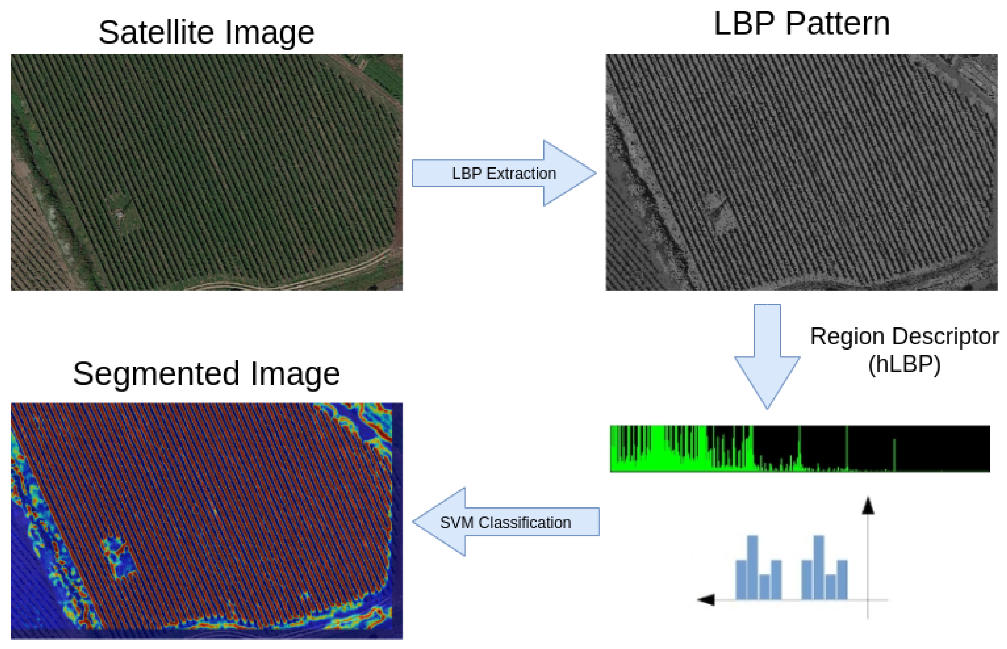
3. Agrobpp-Bridge: Agrob Vineyard Detector

The segmentation task of vineyards in satellite images is divided into two stages: detection of a full vineyard crop in satellite images, and segmentation of paths and vine vegetation to construct a prior occupation grid map. The first stage was performed in a previous work [40] recurring to an SVM classifier. Now, in the second stage, we bench-marked two segmentation tools: “AgRob vineyard Detector”, our developed SVM tool, and “Semantic Segmentation Suite”, a state of the art framework with Tensorflow.
AgRob Vineyard Detector is the developed framework that contains an annotation tool to create image datasets and a segmentation tool. We considered a two classes classification problem: “Vineyard” and “Path” (not “Vineyard”).

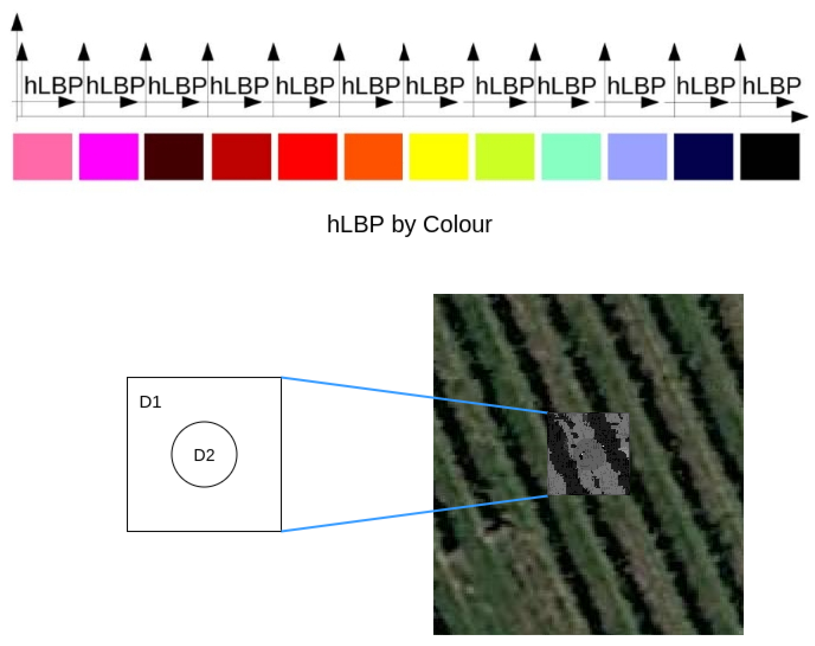
3.1. Segmentation Tool

For the segmentation process, we use an SVM classifier that runs on Robot Operation System (ROS) (http://www.ros.org/.). The input of this tool is a region descriptor extracted from the image. Based on the training step, the SVM tool is able to classify the image pixels according to a class object. Figure 1 depicts the information stream of the classification process.
The region descriptor is based in Local Binary Pattern codes (LBP), a grey-level invariant texture primitive. Ojala et al. [41] presented the non-parametric LBP operator for textured image description. Originally, the LBP uses a grid of 3 × 3 pixels for an arbitrary pixel over an input grey-level image. The LBP code is computed by comparing the grey-level value of the centre pixel and its neighbors within the respective grid. The pixels that are not covered by the grids are estimated by interpolation. Then, the LBP code is a binary number which results from a threshold stage concerning the centre pixel. The image texture is described with an LBP histogram (hLBP), built from all binary pattern of each image pixel as shown in Equation (1), where K is the maximal LBP pattern value. Based on hLBP, we considered the descriptor hLBP by color, as in Figure 2, which contains one LBP histogram per color, discretizing the color ranges into n colors in RGB (Red, Green and Blue) space. With this descriptor, each pixel is related to a color range, which will increment the histogram bin related to the LBP code extracted for that pixel. This descriptor will feed the SVM classifier. Here, the descriptor was modified to optimize the detection in vineyards. So, we concatenated the two descriptors, as shown in Figure 2, to describe the centre and its surroundings. The proposed descriptor considers histograms to describe patterns (LBP) and color. The vineyard rows and the path rows—where machinery/robots can move—have different patterns and colors, which can be easily captured by the presented descriptor. Theoretically, this should work for any permanent woody crops (e.g., Orchards or Olive Groves) because the cultures are disposed in rows (linear and/or contour lines), and the paths are aligned to these rows. However, to extend this work to other agricultural contexts, an extension to the dataset and SVM training may be required. For example, crops with paths with exposed soils (without vegetation), where the soil may have another color, would require this procedure.
H ( k ) = m = 1 M n = 1 N f ( L B P P , R ( m , n ) , k ) ,       k [ 0 , K ] f ( x , y ) = 1 , x = y 0 , o t h e r w i s e .
SVM is a traditional machine learning technique for classification problems. Despite being adequate for binary classification, some approaches decompose the problem into a series of two-class problems [42], allowing SVM to perform multi-class classification. The SVM concept implements the following idea: input vectors are non-linearly mapped to a high-dimension feature space, where a linear decision surface is constructed [43]. Considering a problem of separating the training data ( x 1 , y 1 ) , ( x m , y m ) into two classes, where x i is a feature vector and y i { 1 , + 1 } its class label. Assuming that a hyperplane can separate the two classes, w · x + b = 0 in some space ℍ, the optimal hyperplane will maximize the margin. Change et al. [44] provides a deeper explanation about the SVM theory and its variant libSVM.

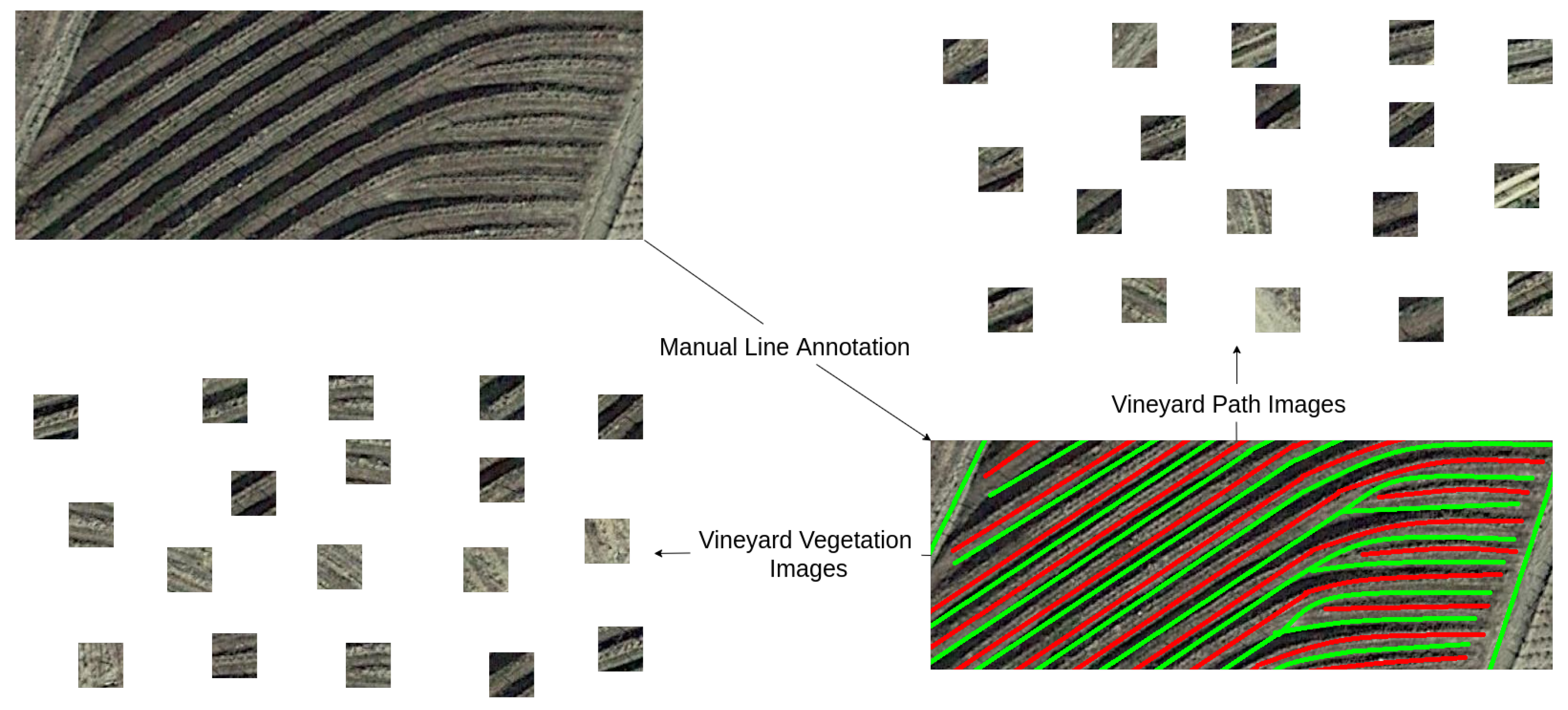
3.2. Annotation Tool

The annotation tool consists of a semi-automatic framework developed to ease the creation of training images datasets of vineyards in satellite images. A training dataset is composed of a set of images with a fixed resolution containing examples of images belonging to a specific class. In this case, there is a group of vineyard vegetation images and another group with vineyard paths images. The process of manually annotating these images is time-consuming and can lead to incorrect class annotations, which will decrease the accuracy of the segmentation process. So, as this process is based on the detection of vineyard lines, our annotation tool requires the user to manually draw a set of lines representing the vegetation and path lines of the vineyard, using any image editing tool (i.e., GIMP (https://www.gimp.org/) or Paint). The annotation tool will create a set of training images based in the line annotations with specified window size, as in Figure 3. This process can also be very time-consuming in the case of large irregular fields. Still, the method is always simpler than a complete manual annotation. In this case, with an annotation made entirely by hand, the user would have to select hundreds or thousands of images with pre-defined window size.
The selection of the window size is crucial and depends upon several factors, such as the image resolution and the distance between vine-trees. If this parameter is not correctly defined, an entirely new dataset can be created with our annotation tool in just a few seconds. If we considered a full manual annotation, the entire process would have to be restarted. Ideally, the size of this window should be enough to cover two vineyard lines. The distance between vineyard rows changes significantly between farms, and satellite images have very different resolutions. So, we have applied the fast Fourier transform (FFT) on the input images to obtain the distance between crop tree rows (in pixels units) and used this value to scale our descriptor window according to the image resolutions and distance between crop trees rows. An FFT is an algorithm that computes the discrete Fourier transform (DFT) of a sequence. Fourier analysis converts a signal from its original domain (in this work, pixels space) to a representation in the frequency domain. The higher frequency with high magnitude is correlated to the crop row spacing. So, to estimate the space between two consecutive vine lines, we calculate the Fast Fourier Transform (FFT) of various columns and rows of a grey-scale version of the image. As represented in Figure 4, eight FFT from four different columns and rows are calculated.
To estimate the desired width, the steps below are executed several times, which will provide different measurements, presenting to the user an average value and the value obtained at each estimation.
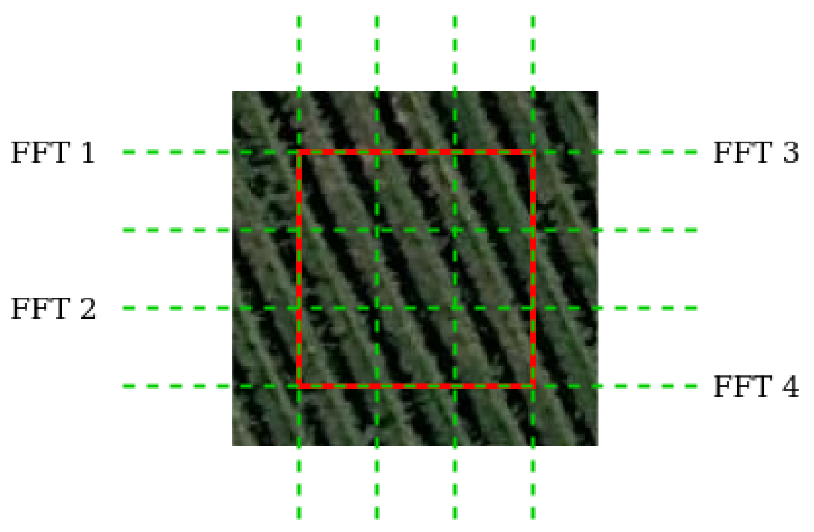
  • Choose a column and a row of the selected image zone and calculate their FFTs.
  • Choose the FFT with maximum magnitude value at the maximum index as this will be closer to the heading of the image.
  • Calculate the distance between two lines: w i d t h = F F T s i z e I n d e x m a x .

3.3. Segmentation Semantic Suite

The Segmentation Semantic Suite [13] is an open-source tool constructed to quickly implement, train and test semantic segmentation models in TensorFlow. Tensorflow is one of the most popular Deep Learning (DL)-oriented frameworks. It allows to create, train, and execute models that can be transferred to heterogeneous devices. With Tensorflow, Convolutional Neural Networks (CNNs) can be used to perform image classification, object detection, and semantic segmentation. This segmentation tool performs automatic data augmentation, a process to enlarge the training dataset by applying a series of random transformations to the original images, such as rotation and translation. It also includes various state-of-the-art models for feature extraction, such as MobileNetV2 [45] and ResNet50/101/152 [46], as well as several segmentation models, like Mobile UNet [47] and Fully Convolutional DenseNet [48]. For the case study of this article, we considered the frontend feature extractor ResNet101 and the segmentation model FC-DenseNet103.

4. AgRobPP-Bridge—AgRob Grid Map to Topologic

AgRob Grid Map to Topologic is a framework developed to deal with big dimensions maps in autonomous robot navigation. As mentioned in our previous work [12], path planning in terrains with large dimensions is complex in terms of memory. This approach automatically divides an occupation grid map into smaller zones and finds the different possible connections between those places. Then, this information is saved into a graph struct, which allows the usage of a search algorithm to find the best possible transaction between two zones. In the resulting graph struct, a vertex represents a delimited place of the map, and an edge represents the connection between to vertices containing information about the Euclidean distance, as in Figure 5.
A typical A* search algorithm, in which pseudo-code is represented in Algorithm 1, was the choice to perform the search between two nodes in the graph space. With this, the large map gets reduced to the strictly necessary zones to navigate between two different places. Considering this method, the amount of computational memory gets substantially reduced.
Algorithm 1 A* algorithm [39]
1: Add origin node to O (Open list)
2: Repeat
3: Choose nbest (best node) from O so that f ( n b e s t ) f ( n ) n O
4: Remove nbest from O and add it to C (Closed list)
5: if nbest = target node then end
6: For all x Q ( n b e s t ) which are not in C do:
  if x O then
   Add node x to O
  else if g(nbest) + c(nbest, x) < g(x) then
   Change parent of node x to nbest
7: until O is empty
The topological map concept for steep slopes vineyards had been addressed in a previous work [39]. However, this method was more complex and presented some outliers. For example, there were unnecessary and repetitive connections between different nodes. The resemblance to AgRob Grid Map to Topologic is in the Voronoi diagram. Both methods start with the extraction of a Voronoi diagram, but here the places delimitation follow a more straightforward approach. As already mentioned, the Voronoi diagram consists of the division of the space by Voronoi segments and Voronoi vertices. These segments represent all the points in the plane equidistant to the nearest sites, and the Voronoi vertices are the points equidistant to three or more sites [38]. Our previous approach started the construction of the topological map by defining a circle in each Voronoi vertice, then filtering these circles to eliminate overlaps. Until this point, the process in both methods is similar. While the previous work used Voronoi segments to find the connection between circles and resorted to parametric equations for the space delimitation process, the current approach is more simplistic, efficient, and effective, as will be explained below. The result of this method will provide us with a map sub-divided into smaller places, with the possible connections between these zones saved in a data structure. Furthermore, an A* search algorithm is available to search for the best transition between places, which will be useful for future approaches with path planning algorithms.
For the step by step demonstration of this method, an occupation grid map of a simulated steep slope vineyard will be considered, as in Figure 6, where the white color represents a free cell and black color an occupied cell. This image is the result of a 2D projection of the simulated 3D model of a steep slope vineyard created with a modeling software in previous work [11].

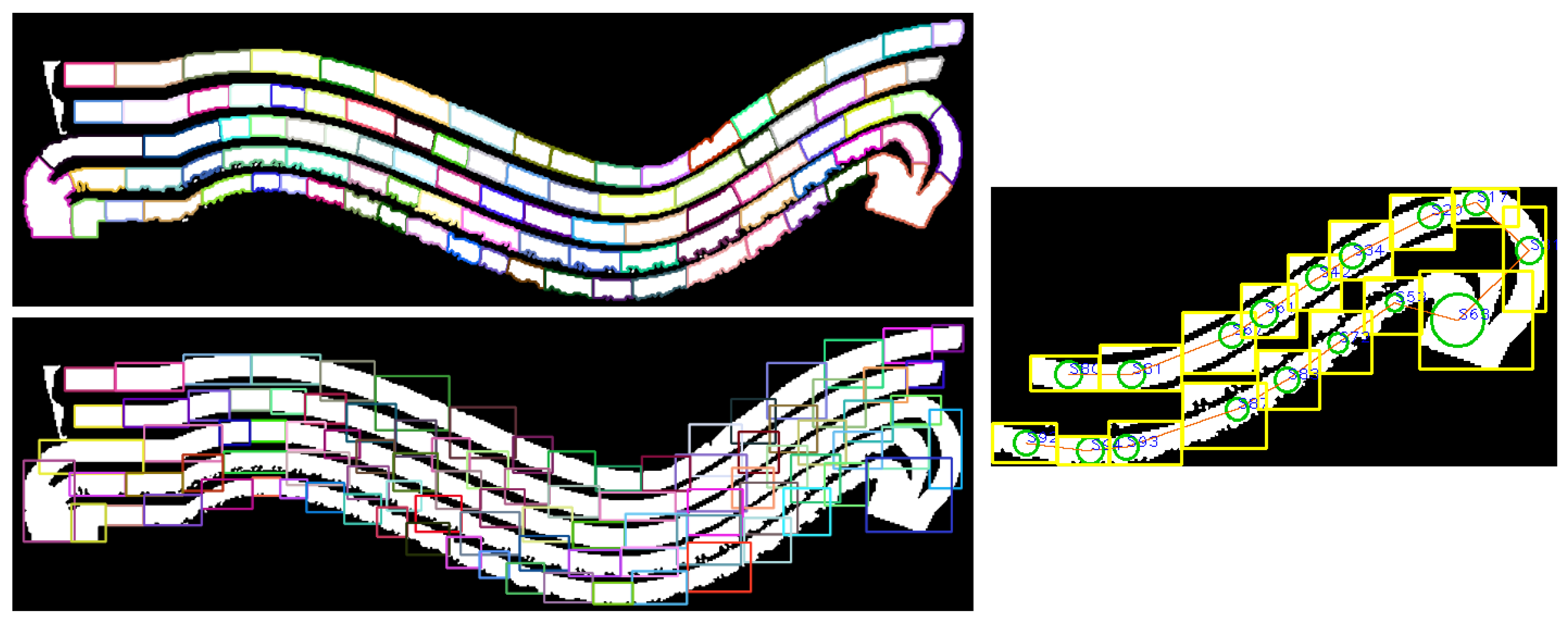
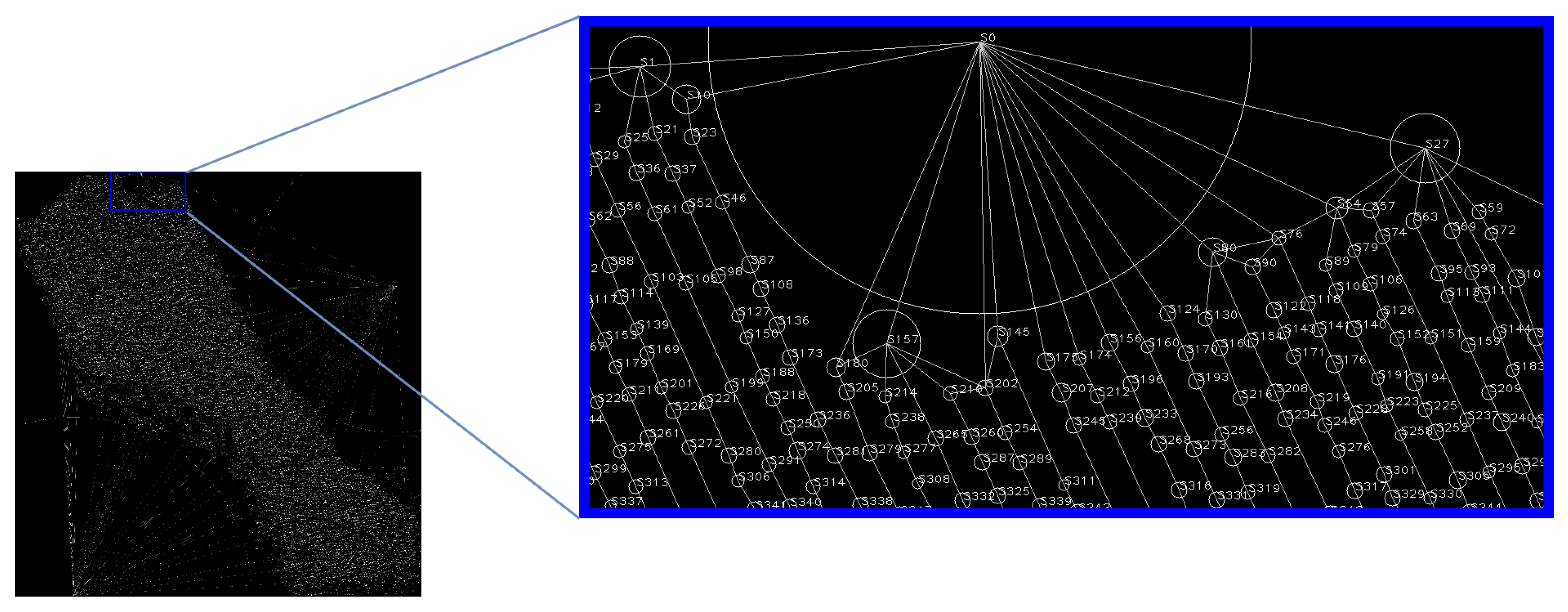
4.1. Voronoi Diagram Extraction

The resulting vertices and segments of the Voronoi diagram are represented in Figure 7. Its construction originates from a beforehand distance map, which contains the Euclidean distance of every cell to the closest obstacle. The development of the algorithm was based on the work of Lau et al. [49].

4.2. Topological Map Construction

The visualisation of the topological map is composed of a set of interconnected circles. Each circle represents a certain zone of the map, that it’s connected to the nearest possible circles, according to the occupation grid map. To construct it, the algorithm associates two parameters to each one of the Voronoi vertices, to define a circle: the circle location r c = ( x c , y c ) that is the same as the Voronoi Vertex, and the circle radius through the distance map, r c = m a p d i s t ( x c , y c ) . With this circle, the algorithm checks, in all of the remaining stored circles, the following condition: r c ( i ) + r c > = ( x c x c ( i ) ) 2 + ( y c y c ( i ) ) 2 . If the condition is true, the circle with a smaller radius is erased. The result of this operation is illustrated in Figure 8.
The next step consists of finding the connections between the circles. For that operation, all the pixels of each circle will have associated a unique label. Then, all the pixels containing a label are expanded until a different label is found. This operation is similar to a recursive process of a morphological operation of erosion until there are no more pixels without a label associated. The result is visible in Figure 9.
With this image, the process of finding the connections between the circles is simple. It is just necessary to check the zones where the label changes. So, a topological map is constructed and represented in Figure 10.

4.3. Place Delimitation

In this stage, the algorithm takes advantage of the expansion performed before, as in Figure 9, to define delimited places on the map. Then, these places are approximated to the nearest possible rectangle, and this information is saved into the graph struct. At this stage, it is possible to use A* search algorithm to find the best transition sequence between two different nodes. The result of this operation is visible in Figure 11, where A* was used to find the connection between the nodes S80 and S92. The final result presents a map that only contains the strictly necessary zones for robotic navigation between those two nodes.

5. Results

This section presents the results of AgRobPP-bridge. The mentioned segmentation methods, AgRob Vineyard Detector and Segmentation Semantic suite are demonstrated in two different vineyards to extract an Occupancy Grid Map. AgRob Grid Map to Topological map extraction is demonstrated with one of the extracted grid maps. The satellite images of the vineyards are publicly available on Google Maps, and we resorted to a public tool [50] to obtain high-resolution images with the necessary dimensions to cover an entire vineyard. One of the vineyards, as in Figure 12A, is a flat vineyard located at “Quinta da Aveleda” (41.205074, −8.307765), with an area of approximately 5.2 hectares. The other image, Figure 12B, corresponds to a portion of a steep slope vineyard located at “Quinta do Seixo” (41.167574, −7.553293) with an approximated area of 2.3 hectares. Both images were acquired at the maximum possible resolution with 300 pixels per inch.

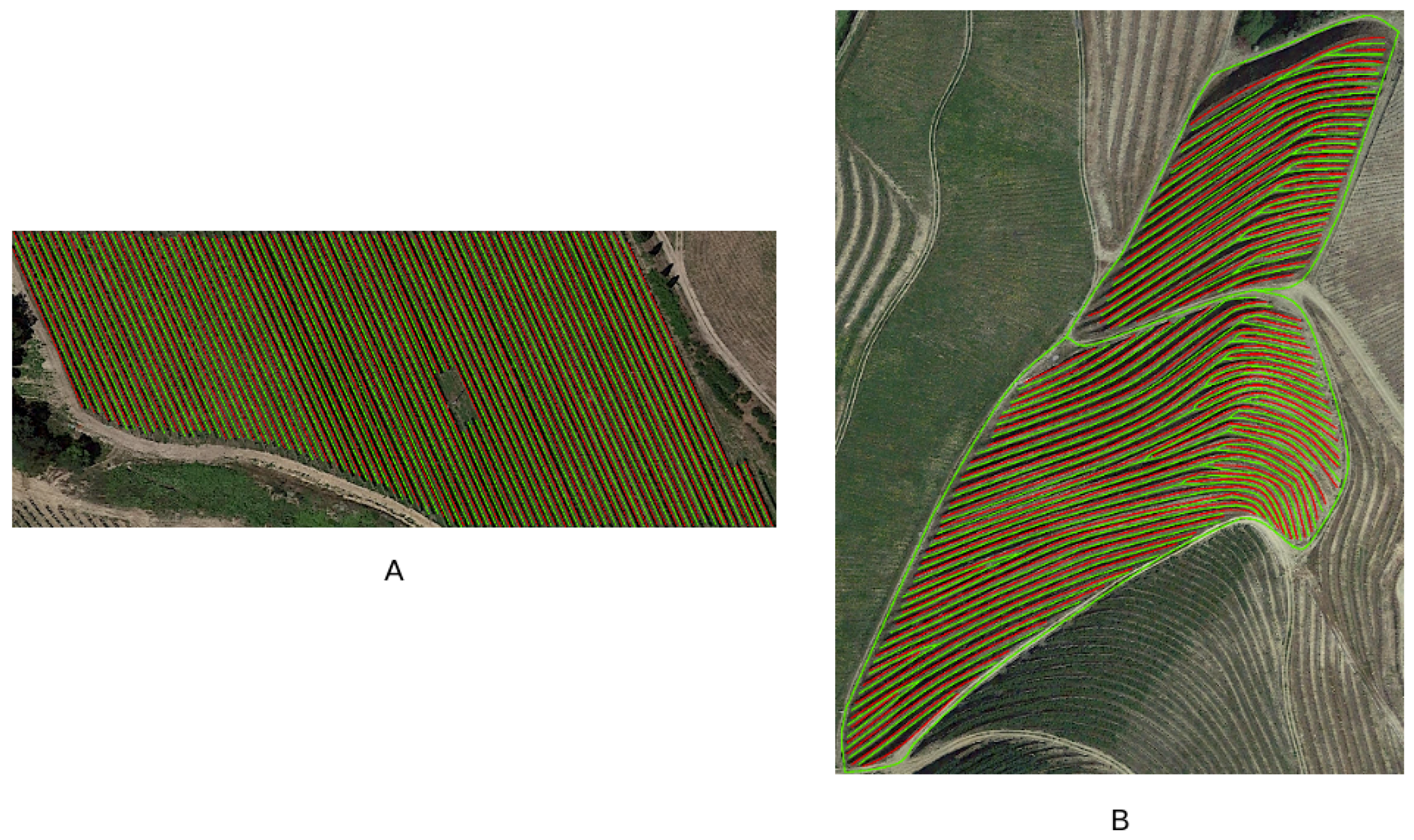
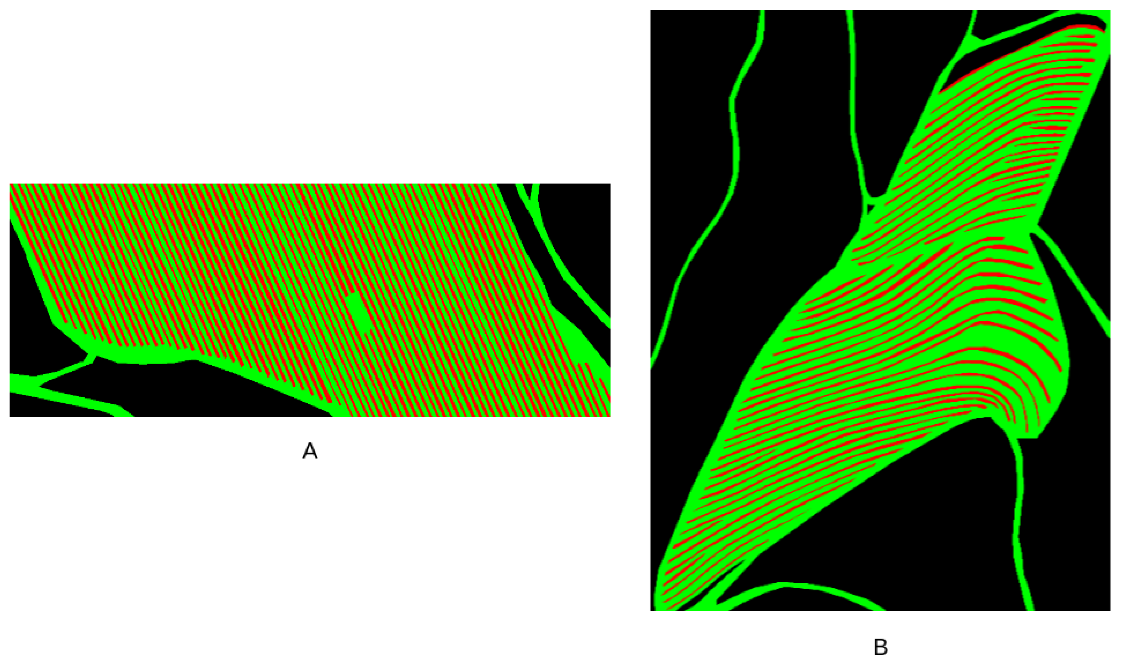
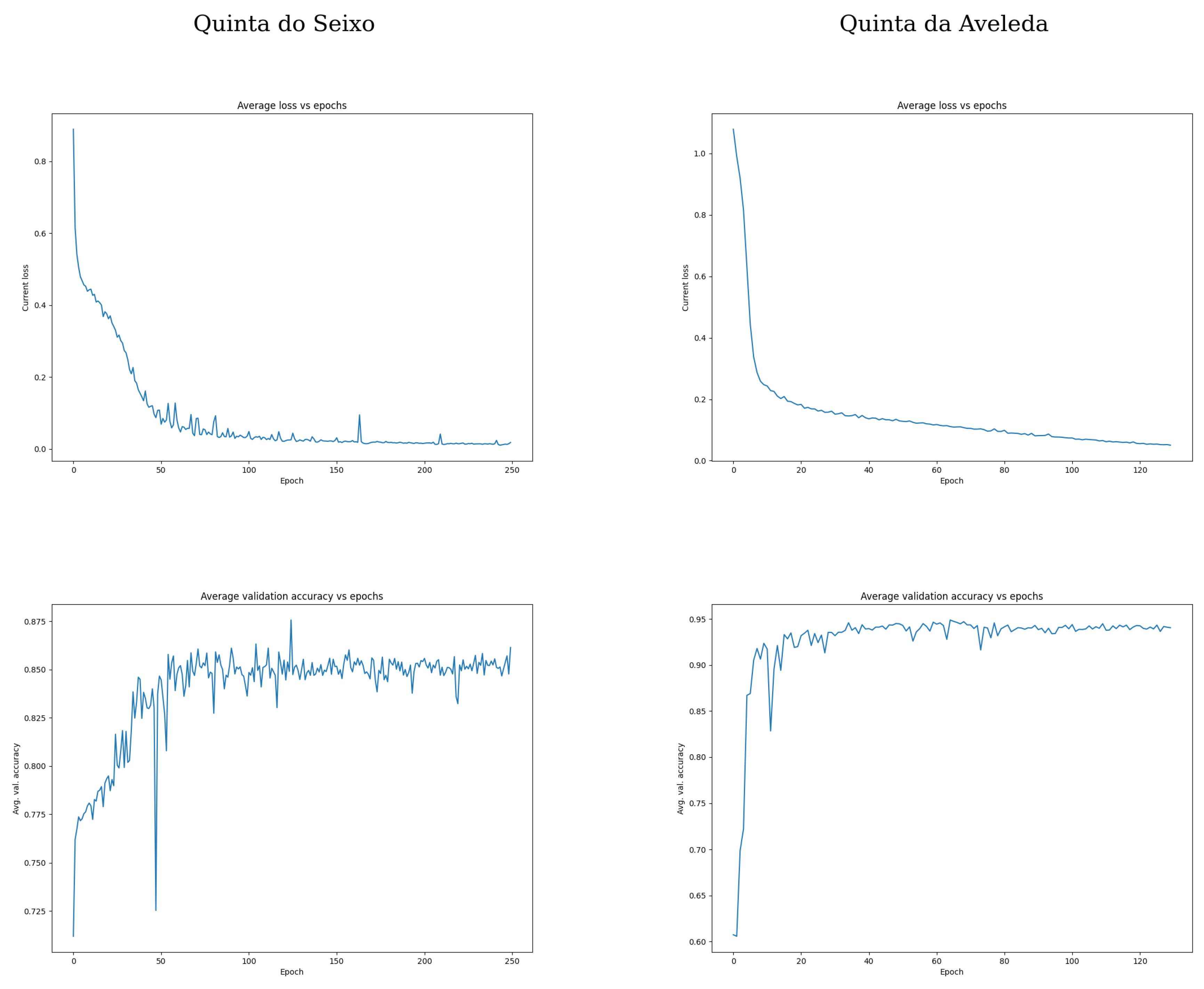
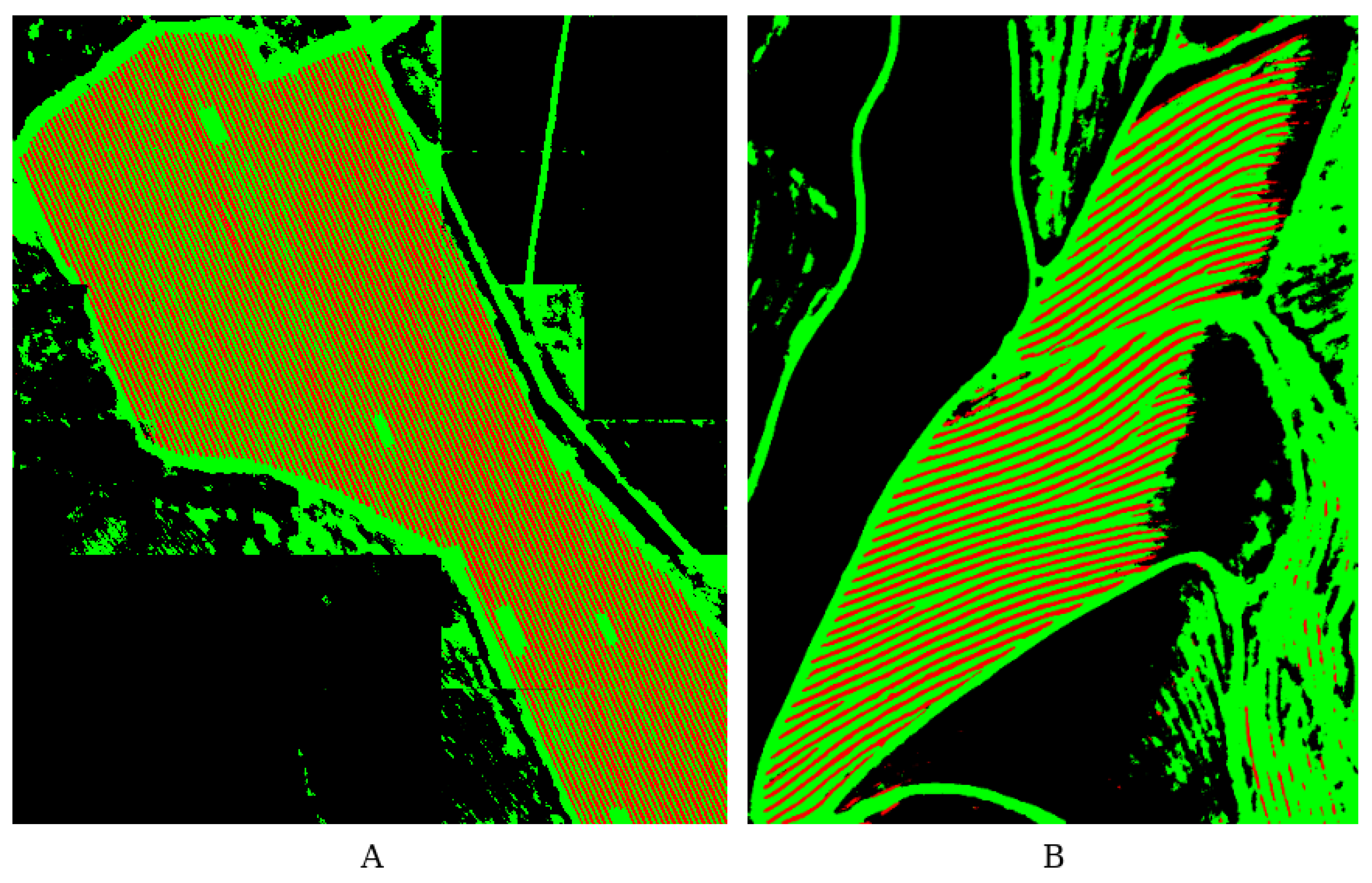
5.1. Agrob Vineyard Detector Results

Two different training datasets were created with the annotation tool mentioned in Section 3.2, visible in Figure 13. The dataset contains two classes: “Vineyard” which includes the vine-trees, and “Path” that represents everything else. Although the class “Not Vineyard” may not necessarily include a path for robotic navigation, the main goal is to identify the vineyards. As SVM is a tool more suitable for binary classification, we simplified the problem to work with just these two classes. For the vineyard of “Quinta da Aveleda”, we annotated a portion of the image with a window size of 70 × 70 pixels. The annotation on the steep slope vineyard was performed with a window of 45 × 45 pixels. The SVM tests were performed in Ubuntu 18.04.3 LTS under ROS Melodic framework, in a computer with Intel(R) Core(TM) i7-8750H CPU @ 2.20GHz × 12, 16 GB of memory. The application runs in CPU without any parallelization.
The accuracy results of the training process are expressed in Table 1 with a confusion matrix. About 15% of the images in the dataset are used to test the training process. The confusion matrix table indicates, for example, that, in 102 images belonging to “vineyard”, 4 were wrongly classified as “path”. Ideally, the values outside of the main diagonal of a confusion matrix should be 0.
The images in Figure 14 represent the SVM segmentation result with the flat vineyard at “Quinta da Aveleda” and the corresponding Occupancy Grid Map. The result in the steep slope vineyard is shown in Figure 15. The result is present in the form of a color map, which is related to the probability of each pixel to belong to the class “Vineyard Path”, where blue represents the lowest probability and red the highest. The grid map is obtained through a threshold process in the color map image. Two ground truth images were created, similar to the images in Figure 16 to calculate the accuracy of the method. These images were compared pixel by pixel to the final result of the SVM tool in order to determine quality metrics. Table 2 presents the Accuracy and the metric F1-score, common in binary classification problems. This table is similar to a confusion matrix (Table 1), but, instead of presetting the number of images correctly identified, it considers the number of pixels by comparing the image to a ground-truth image. However, such data is not available, so we annotated the images manually and consider them as ground-truth, as in Figure 16. For the accuracy, we consider all the pixels correctly identified out of all pixels in the image. F1-score combines “Precision” and “Recall” metrics with a harmonic average. “Recall” refers to the number of pixels correctly identified as Positive (Vineyard) out of the total True positives (“Vineyard” and false “Path”). The “Precision” is the number of items correctly identified as positive (“Vineyard”) out of all pixels identified as positives (“Vineyard” and false “Vineyard”) [51].

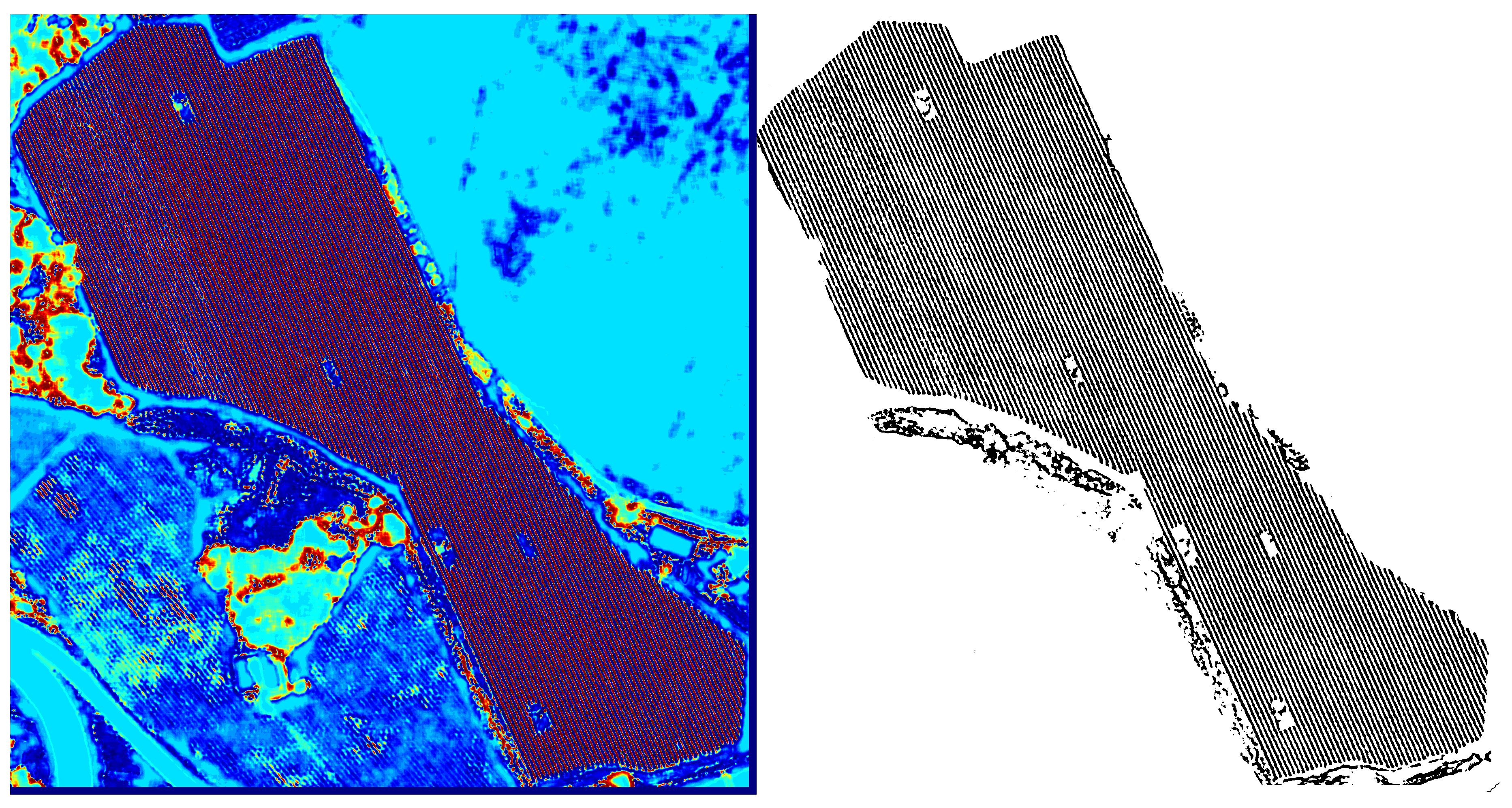
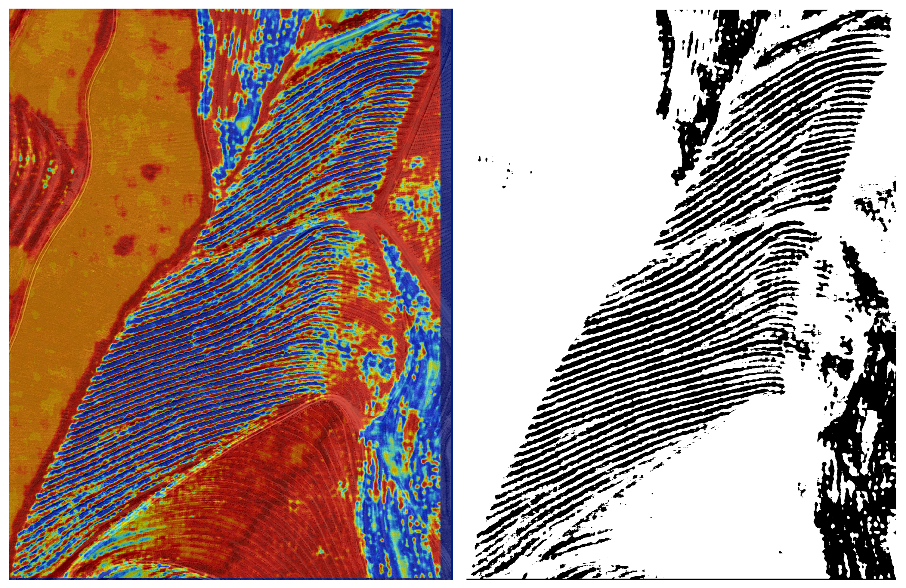
5.2. Segmentation Semantic Suite Results

To compare the results of this tool with the SVM classifier, we created two training datasets using similar information sources, that is, using the same area of satellite images. Here the annotation process was manual and time-consuming because it must be performed to every individual pixel. Each pixel gets associated with a particular color, which is related to a specific class. We considered three classes: Vineyard, Path, and Background. The last one represents everything that is outside of the first two classes. The annotation is illustrated in Figure 16.
Two training processes were performed, and the graphics correlating the average loss and average accuracy with the number of epochs are visible in Figure 17. The prediction results are revealed in Figure 18, and Table 3 presents the accuracy and F1-Score of the prediction similarly to Table 2. The classes Path and Background were considered to be one single class (“Not Vineyard”) to calculate the F1-score. This application requires a GPU, so we ran these tests remotely with Google Colab Platform (https://colab.research.google.com).

5.3. Agrob Grid Map to Topologic Results

The results for this tool were demonstrated along Section 4 considering a simulated map of a steep slope vineyard. The present section presents the results of this tool applied to the occupation grid map obtained in the segmentation of “Quinta da Aveleda” vineyard, as in Figure 15, as this is the most complete grid map with the biggest area. As the image dimensions of the maps are considerable, 6490 × 6787 pixels, it is only possible to highlight part of the result. Figure 19 shows the resulting topological represented by circles and their connections. The place delimitation operation is illustrated in Figure 20. Then, we present an example of a path search operation between two nodes using A* search algorithm in Figure 21.

5.4. Results Discussion

The presented results of satellite image segmentation and topological map extraction are satisfactory. It is possible to extract an occupation grid map from satellite images and create a topological map with the results of the segmentation. The developed SVM (AgRob Vineyard Detector) tool demonstrated a similar performance when compared to a Deep Learning alternative using Semantic Segmentation Suite. Each approach has different characteristics, and Table 4 presents a small benchmark between these methods according to the experience of this work. The training time with the SVM tool takes less than one minute, while, with the deep learning tool, this time can reach several hours, even with the process parallelized in a GPU. Such a thing does not happen in AgRob Vineyard Detector, which is running sequentially in CPU without any parallelization. However, the testing time that takes some seconds with the Semantic Segmentation Suite took about two hours in some of our experiences with the SVM tool. Nevertheless, as already mentioned, this tool is not optimized to reduce the processing time. The annotation process with the Deep Learning approach may be the main drawback. As the tool requires a pixel to pixel annotation, the process was performed manually and took about three hours in each image to be completed. The same process in the SVM took less than one hour, with the help of the annotation tool described in Section 3.2. The precision in both cases is acceptable, even though we are missing a real ground-truth image to make a proper evaluation. The accuracy in the two methods is higher than 73% and reaches 89%, but the F1-Score drops significantly in the SVM tool. This is happening because the precision of the class vineyard is lower than the class “Path”, as visible in Table 2. Such phenomena may be occurring due to the use of a manually annotated image as ground-truth. 80% of the pixels in the ground-truth image marked as vineyard were correctly identified, but this tool identified more extensive lines, which causes the precision to decrease. So, the decrease in F1-score may be caused by human error during the annotation process. With this experience, it could be concluded that AgRob Vineyard Detector is simpler to use and that there are no substantial gains in using the alternative framework. However, such claim can not be fully accepted without a proper evaluation of the data using an accurate ground-truth image. The AgRob Grid Map to Topologic tool revealed good results even when tested in a map with considerable big dimensions. Without this, a path planning algorithm would have to deal with a vast map of 6490 × 6787 pixels to perform a simple operation of finding a path between two near sites. This operation could cause memory problems and affect the performance of the path planning algorithm. Using the topological tool, and considering the most simplistic approach, the path planning tool would work with a much smaller map of 427 × 551 pixels, which represents a reduction of 99.5% of the area.

6. Conclusions

The proposed work presented an approach to deal with big dimensions of agricultural terrain in robotic path planning. For such purpose, we proposed the AgRobPP-bridge, a method to extract an Occupation Grid Map from a satellite image and a tool to construct a topological map from a Grid Map. Based on an SVM classifier, AgRoB Vineyards Detector identifies Vineyards from satellite images and produces an Occupation Grid Map. This tool was bench-marked with an alternative open-source framework, Semantic Segmentation Suite, which is constructed to implement, train, and test segmentation models in TensorFlow. The experience indicated that AgRoB Vineyards Detector is simpler to use, requires less computational resources, and gives a similar accuracy when compared with Semantic Segmentation Suite. However, as there is not a real ground-truth image, it is not possible to assure a reliable precision metric. For this purpose, the results were compared with a manually annotated image, being that, the resolution is not sufficient to ensure correct annotations. To the construction of the topological map began with the extraction of a Voronoi diagram, ending with the map with delimited places saved in a graph structure, with a simple A* search algorithm to find the best transition between different places. The experiments showed promising results when dealing with significant large maps. The tool is capable to efficiently extract the topological map, delimit the areas according to the nodes of the topological map, and search for a transition path between two different nodes. As future work, we will test the segmentation tool with higher resolution images obtained from a drone or an aeroplane and construct a reliable ground-truth image using land sensors from a ground robot. The topological tool will be applied to a path planning framework in order to solve computation memory problems when dealing with big maps.

Author Contributions

Conceptualization, L.C.S. and F.N.S.; methodology, L.C.S., F.N.S. and A.S.A.; software, L.C.S., F.N.S. and A.S.A.; validation, L.C.S. and F.N.S.; formal analysis, F.N.S., A.V., A.S.A. and M.P.; investigation, L.C.S., F.N.S. and A.S.A.; resources, F.N.S.; data curation, L.C.S.; Writing—Original draft preparation, L.C.S.; Writing—Review and editing, F.N.S., M.P., L.C.S., A.S.A. and A.V.; supervision, F.N.S. and A.V.; project administration, F.N.S.; funding acquisition, F.N.S. All authors have read and agreed to the published version of the manuscript.

Funding

This work is financed by the ERDF—European Regional Development Fund through the Operational Programme for Competitiveness and Internationalisation—COMPETE 2020 under the PORTUGAL 2020 Partnership Agreement, and through the Portuguese National Innovation Agency (ANI) as a part of project ROMOVI: POCI-01-0247-FEDER-017945.

Conflicts of Interest

The authors declare no conflict of interest.

Abbreviations

The following abbreviations are used in this manuscript:
SLAMSimultaneous localization and mapping
LBPLocal binary patterns
SVMSupport vector machine
GNSSGlobal navigation satellite systems
AgRobPPAgricultural robotics path planning
LIDARLight detection and ranging
UAVUnmanned aerial vehicle
ROSRobot operating system
FFTFast Fourier transform
DFTDiscrete Fourier transform
DLDeep learning
CNNConvolutional neural network
CPUCentral processing unit
GPUGraphical processing unit

References

  1. Kitzes, J.; Wackernagel, M.; Loh, J.; Peller, A.; Goldfinger, S.; Cheng, D.; Tea, K. Shrink and share: Humanity’s present and future Ecological Footprint. Philos. Trans. R. Soc. B Biol. Sci. 2008, 363, 467–475. [Google Scholar] [CrossRef] [PubMed] [Green Version]
  2. Perry, M. Science and Innovation Strategic Policy Plans for the 2020s (EU,AU,UK): Will They Prepare Us for the World in 2050? Appl. Econ. Financ. 2015, 2, 76–84. [Google Scholar] [CrossRef]
  3. Leshcheva, M.; Ivolga, A. Human resources for agricultural organizations of agro-industrial region, areas for improvement. In Sustainable Agriculture and Rural Development in Terms of the Republic of Serbia Strategic Goals Realization within the Danube Region: Support Programs for the Improvement of Agricultural and Rural Development, 14–15 December 2017, Belgrade, Serbia. Thematic Proceedings; Institute of Agricultural Economics: Belgrade, Serbia, 2018; pp. 386–400. [Google Scholar]
  4. Rica, R.L.V.; Delan, G.G.; Tan, E.V.; Monte, I.A. Status of agriculture, forestry, fisheries and natural resources human resource in cebu and bohol, central philippines. J. Agric. Technol. Manag. 2018, 19, 1–7. [Google Scholar] [CrossRef]
  5. Robotics, E. Strategic Research Agenda for Robotics in Europe 2014–2020. Available online: Eu-robotics.net/cms/upload/topicgroups/SRA2020SPARC.pdf (accessed on 21 April 2018).
  6. Bietresato, M.; Carabin, G.; D’Auria, D.; Gallo, R.; Ristorto, G.; Mazzetto, F.; Vidoni, R.; Gasparetto, A.; Scalera, L. A tracked mobile robotic lab for monitoring the plants volume and health. In Proceedings of the 2016 12th IEEE/ASME International Conference on Mechatronic and Embedded Systems and Applications (MESA), Auckland, New Zealand, 29–31 August 2016; pp. 1–6. [Google Scholar]
  7. Ristorto, G.; Gallo, R.; Gasparetto, A.; Scalera, L.; Vidoni, R.; Mazzetto, F. A Mobile Laboratory for Orchard Health Status Monitoring in Precision Frming. In Proceedings of the XXXVII CIOSTA & CIGR Section V Conference, Research and innovation for the Sustainable and Safe Management of Agricultural and Forestry Systems, Palermo, Italy, 13–15 June 2017. [Google Scholar]
  8. Mahmud, M.S.A.; Abidin, M.S.Z.; Mohamed, Z.; Rahman, M.K.I.A.; Iida, M. Multi-objective path planner for an agricultural mobile robot in a virtual greenhouse environment. Comput. Electron. Agric. 2019, 157, 488–499. [Google Scholar] [CrossRef]
  9. Iqbal, J.; Xu, R.; Sun, S.; Li, C. Simulation of an Autonomous Mobile Robot for LiDAR-Based In-Field Phenotyping and Navigation. Robotics 2020, 9, 46. [Google Scholar] [CrossRef]
  10. Fountas, S.; Mylonas, N.; Malounas, I.; Rodias, E.; Hellmann Santos, C.; Pekkeriet, E. Agricultural Robotics for Field Operations. Sensors 2020, 20, 2672. [Google Scholar] [CrossRef] [PubMed]
  11. Dos Santos, F.N.; Sobreira, H.; Campos, D.; Morais, R.; Moreira, A.P.; Contente, O. Towards a reliable robot for steep slope vineyards monitoring. J. Intell. Robot. Syst. 2016, 83, 429–444. [Google Scholar] [CrossRef]
  12. Santos, L.; Santos, F.; Mendes, J.; Costa, P.; Lima, J.; Reis, R.; Shinde, P. Path Planning Aware of Robot’s Center of Mass for Steep Slope Vineyards. Robotica 2020, 38, 684–698. [Google Scholar] [CrossRef]
  13. Seif, G. Semantic Segmentation Suite in TensorFlow. Available online: https://github.com/GeorgeSeif/Semantic-Segmentation-Suite (accessed on 15 July 2020).
  14. Raja, P.; Pugazhenthi, S. Optimal path planning of mobile robots: A review. Int. J. Phys. Sci. 2012, 7, 1314–1320. [Google Scholar] [CrossRef]
  15. Mac, T.T.; Copot, C.; Tran, D.T.; De Keyser, R. Heuristic approaches in robot path planning: A survey. Robot. Auton. Syst. 2016, 86, 13–28. [Google Scholar] [CrossRef]
  16. Galceran, E.; Carreras, M. A survey on coverage path planning for robotics. Robot. Auton. Syst. 2013, 61, 1258–1276. [Google Scholar] [CrossRef] [Green Version]
  17. Pivtoraiko, M.; Knepper, R.A.; Kelly, A. Differentially constrained mobile robot motion planning in state lattices. J. Field Robot. 2009, 26, 308–333. [Google Scholar] [CrossRef]
  18. Karaman, S.; Walter, M.R.; Perez, A.; Frazzoli, E.; Teller, S. Anytime Motion Planning using the RRT*. In Proceedings of the 2011 IEEE International Conference on Robotics and Automation, Shangai, China, 9–13 May 2011; pp. 1478–1483. [Google Scholar]
  19. Fernandes, E.; Costa, P.; Lima, J.; Veiga, G. Towards an orientation enhanced astar algorithm for robotic navigation. In Proceedings of the 2015 IEEE International Conference on Industrial Technology (ICIT), Seville, Spain, 17–19 March 2015; IEEE; pp. 3320–3325. [Google Scholar]
  20. Elhoseny, M.; Tharwat, A.; Hassanien, A.E. Bezier curve based path planning in a dynamic field using modified genetic algorithm. J. Comput. Sci. 2018, 25, 339–350. [Google Scholar] [CrossRef]
  21. Santos, L.C.; Santos, F.N.; Solteiro Pires, E.J.; Valente, A.; Costa, P.; Magalhães, S. Path Planning for ground robots in agriculture: A short review. In Proceedings of the 2020 IEEE International Conference on Autonomous Robot Systems and Competitions (ICARSC), Ponta Delgada, Azores, Portugal, 15–17 April 2020; pp. 61–66. [Google Scholar]
  22. Mougel, B.; Lelong, C.; Nicolas, J. Classification and information extraction in very high resolution satellite images for tree crops monitoring. In Remote Sensing for a Changing Europe, Proceedings of the 28th Symposium of the European Association of Remote Sensing Laboratories, Istanbul, Turkey, 2–5 June 2008; IOS Press: Amsterdam, The Netherlands, 2009; pp. 73–79. [Google Scholar]
  23. Karakizi, C.; Oikonomou, M.; Karantzalos, K. Vineyard detection and vine variety discrimination from very high resolution satellite data. Remote Sens. 2016, 8, 235. [Google Scholar] [CrossRef] [Green Version]
  24. Rovira-Más, F.; Zhang, Q.; Reid, J.; Will, J. Hough-transform-based vision algorithm for crop row detection of an automated agricultural vehicle. Proc. Inst. Mech. Eng. Part D J. Automob. Eng. 2005, 219, 999–1010. [Google Scholar] [CrossRef]
  25. Pérez-Ortiz, M.; Gutiérrez, P.A.; Peña, J.M.; Torres-Sánchez, J.; López-Granados, F.; Hervás-Martínez, C. Machine learning paradigms for weed mapping via unmanned aerial vehicles. In Proceedings of the 2016 IEEE Symposium Series on Computational Intelligence (SSCI), Athens, Greece, 6–9 December 2016; IEEE; pp. 1–8. [Google Scholar]
  26. Delenne, C.; Durrieu, S.; Rabatel, G.; Deshayes, M. From pixel to vine parcel: A complete methodology for vineyard delineation and characterization using remote-sensing data. Comput. Electron. Agric. 2010, 70, 78–83. [Google Scholar] [CrossRef] [Green Version]
  27. Smit, J.; Sithole, G.; Strever, A. Vine signal extraction—An application of remote sensing in precision viticulture. S. Afr. J. Enol. Vitic. 2010, 31, 65–74. [Google Scholar] [CrossRef] [Green Version]
  28. Poblete-Echeverría, C.; Olmedo, G.F.; Ingram, B.; Bardeen, M. Detection and segmentation of vine canopy in ultra-high spatial resolution RGB imagery obtained from unmanned aerial vehicle (UAV): A case study in a commercial vineyard. Remote Sens. 2017, 9, 268. [Google Scholar] [CrossRef] [Green Version]
  29. Nolan, A.; Park, S.; Fuentes, S.; Ryu, D.; Chung, H. Automated detection and segmentation of vine rows using high resolution UAS imagery in a commercial vineyard. In Proceedings of the 21st International Congress on Modelling and Simulation, Gold Coast, Australia, 29 November–4 December 2015; pp. 1406–1412. [Google Scholar]
  30. Comba, L.; Gay, P.; Primicerio, J.; Aimonino, D.R. Vineyard detection from unmanned aerial systems images. Comput. Electron. Agric. 2015, 114, 78–87. [Google Scholar] [CrossRef]
  31. Quinta do Seixo at Sogrape. Available online: https://eng.sograpevinhos.com/regioes/Douro/locais/QuintadoSeixo (accessed on 30 August 2020).
  32. Kuipers, B.; Byun, Y.T. A robot exploration and mapping strategy based on a semantic hierarchy of spatial representations. Robot. Auton. Syst. 1991, 8, 47–63. [Google Scholar] [CrossRef]
  33. Luo, R.C.; Shih, W. Topological map Generation for Intrinsic Visual Navigation of an Intelligent Service Robot. In Proceedings of the 2019 IEEE International Conference on Consumer Electronics (ICCE), Las Vegas, NV, USA, 11–13 January 2019; pp. 1–6. [Google Scholar]
  34. Joo, K.; Lee, T.; Baek, S.; Oh, S. Generating topological map from occupancy grid-map using virtual door detection. In Proceedings of the IEEE Congress on Evolutionary Computation, Las Vegas, NV, USA, 11–13 January 2010; pp. 1–6. [Google Scholar]
  35. Thrun, S. Learning metric-topological maps for indoor mobile robot navigation. Artif. Intell. 1998, 99, 21–71. [Google Scholar] [CrossRef] [Green Version]
  36. Brunskill, E.; Kollar, T.; Roy, N. Topological mapping using spectral clustering and classification. In Proceedings of the 2007 IEEE/RSJ International Conference on Intelligent Robots and Systems, San Diego, CA, USA, 29 October–2 November 2007; pp. 3491–3496. [Google Scholar]
  37. Konolige, K.; Marder-Eppstein, E.; Marthi, B. Navigation in hybrid metric-topological maps. In Proceedings of the 2011 IEEE International Conference on Robotics and Automation, Shanghai, China, 9–13 May 2011; pp. 3041–3047. [Google Scholar]
  38. Santos, F.N.; Moreira, A.P.; Costa, P.C. Towards Extraction of Topological maps from 2D and 3D Occupancy Grids. In Progress in Artificial Intelligence; Correia, L., Reis, L.P., Cascalho, J., Eds.; Springer: Berlin/Heidelberg, Germany, 2013; pp. 307–318. [Google Scholar]
  39. Santos, L.; Santos, F.N.; Magalhães, S.; Costa, P.; Reis, R. Path Planning approach with the extraction of Topological maps from Occupancy Grid Maps in steep slope vineyards. In Proceedings of the 2019 IEEE International Conference on Autonomous Robot Systems and Competitions (ICARSC), Porto, Portugal, 24–26 April 2019; pp. 1–7. [Google Scholar]
  40. Santos, L.; Santos, F.N.; Filipe, V.; Shinde, P. Vineyard Segmentation from Satellite Imagery Using Machine Learning. In Progress in Artificial Intelligence; Moura Oliveira, P., Novais, P., Reis, L.P., Eds.; Springer International Publishing: Cham, Switzerland, 2019; pp. 109–120. [Google Scholar]
  41. Ojala, T.; Pietikäinen, M.; Harwood, D. A comparative study of texture measures with classification based on featured distributions. Pattern Recognit. 1996, 29, 51–59. [Google Scholar] [CrossRef]
  42. Liu, Y.; Zheng, Y.F. One-against-all multi-class SVM classification using reliability measures. In Proceedings of the 2005 IEEE International Joint Conference on Neural Networks, Montreal, QC, Canada, 31 July–4 August 2005; IEEE; pp. 849–854. [Google Scholar]
  43. Cortes, C.; Vapnik, V. Support-vector networks. Mach. Learn. 1995, 20, 273–297. [Google Scholar] [CrossRef]
  44. Chang, C.C.; Lin, C.J. LIBSVM: A library for support vector machines. ACM Trans. Intell. Syst. Technol. (TIST) 2011, 2, 1–27. [Google Scholar] [CrossRef]
  45. Sandler, M.; Howard, A.; Zhu, M.; Zhmoginov, A.; Chen, L.C. MobileNetV2: Inverted Residuals and Linear Bottlenecks. In Proceedings of the IEEE Conference on Computer Vision and Pattern Recognition (CVPR), Salt Lake City, UT, USA, 18–23 June 2018. [Google Scholar]
  46. He, K.; Zhang, X.; Ren, S.; Sun, J. Deep Residual Learning for Image Recognition. In Proceedings of the IEEE Conference on Computer Vision and Pattern Recognition (CVPR), Caesars Palace, Las Vegas, NV, USA, 26 June–1 July 2016. [Google Scholar]
  47. Jing, J.; Wang, Z.; Rätsch, M.; Zhang, H. Mobile-Unet: An efficient convolutional neural network for fabric defect detection. Text. Res. J. 2020. [Google Scholar] [CrossRef]
  48. Jegou, S.; Drozdzal, M.; Vazquez, D.; Romero, A.; Bengio, Y. The One Hundred Layers Tiramisu: Fully Convolutional DenseNets for Semantic Segmentation. In Proceedings of the IEEE Conference on Computer Vision and Pattern Recognition (CVPR) Workshops, Honolulu, HI, USA, 21–26 July 2017. [Google Scholar]
  49. Lau, B.; Sprunk, C.; Burgard, W. Improved updating of Euclidean distance maps and Voronoi diagrams. In Proceedings of the 2010 IEEE/RSJ International Conference on Intelligent Robots and Systems, Taipei, Taiwan, 18–22 October 2010; pp. 281–286. [Google Scholar]
  50. Map Puzzel Tool for Google Maps. Available online: http://www.mappuzzle.se/ (accessed on 2 July 2020).
  51. Espejo-Garcia, B.; Lopez-Pellicer, F.J.; Lacasta, J.; Moreno, R.P.; Zarazaga-Soria, F.J. End-to-end sequence labeling via deep learning for automatic extraction of agricultural regulations. Comput. Electron. Agric. 2019, 162, 106–111. [Google Scholar] [CrossRef]
Figure 1. Information flow of the segmentation process.
Robotics 09 00077 g001
Figure 2. Representation of the concatenated descriptor hLBP by Color—D1: descriptor 1; D2—descriptor 2.
Robotics 09 00077 g002
Figure 3. Example usage of the annotation tool.
Robotics 09 00077 g003
Figure 4. Demonstration of calculated fast Fourier transforms (FFTs) in a satellite vineyard image.
Robotics 09 00077 g004
Figure 5. Representation of the graph struct used for the topological map.
Robotics 09 00077 g005
Figure 6. Occupation grid map of simulated steep slope vineyard.
Robotics 09 00077 g006
Figure 7. Vertices and segments of voronoi diagram of simulated steep slope vineyard.
Robotics 09 00077 g007
Figure 8. Filtering of circles in Voronoi vertices: a step on the construction of a topological map.
Robotics 09 00077 g008
Figure 9. Expansion labels of circles in Voronoi vertices.
Robotics 09 00077 g009
Figure 10. Topological map of a simulated steep slope vineyard.
Robotics 09 00077 g010
Figure 11. Space Delimitation and A* search result between nodes S82 and S92.
Robotics 09 00077 g011
Figure 12. Two Vineyards satellite images considered: (A) “Quinta da Aveleda”, (B) “Quinta do Seixo”.
Robotics 09 00077 g012
Figure 13. Annotation of two satellite vineyard images with Annotation tool for SVM: (A) “Quinta da Aveleda”, (B) “Quinta do Seixo”.
Robotics 09 00077 g013
Figure 14. SVM Segmentation results in a color map of the vineyard at Quinta da Aveleda (Left). Resulting Occupancy Grid Map (Right). Black: Vineyard vegetation.
Robotics 09 00077 g014
Figure 15. SVM Segmentation results in a color map of steep slope vineyard at Quinta do Seixo (Left). Resulting Occupancy Grid Map (Right). Black: Vineyard vegetation.
Robotics 09 00077 g015
Figure 16. Annotation of two satellite vineyard images for Semantic Segmentation Suite: (A) Quinta da Aveleda, (B) Quinta do Seixo; Red: Vineyard, Green: Path, Black: Background.
Robotics 09 00077 g016
Figure 17. Relation between Average Loss (Top) and Average accuracy (Bottom) with train epochs on Semantic Segmentation Suite.
Robotics 09 00077 g017
Figure 18. Semantic Segmentation Suite results. (A)“Quinta da Aveleda”, (B)“Quinta do Seixo”.
Robotics 09 00077 g018
Figure 19. Topological map of “Quinta da Aveleda”.
Robotics 09 00077 g019
Figure 20. Place delimitation with the topological map of “Quinta da Aveleda”.
Robotics 09 00077 g020
Figure 21. Transition path between nodes 609 and 594 using the topological map of “Quinta da Aveleda”.
Robotics 09 00077 g021
Table 1. Confusion Matrix of the SVM training process.
Classes
of Images
Train
Images
Test
Images
Confusion MatrixAccuracy
(%)
PathVegetation
AveledaPath5374578072893.4%
Vegetation684582102498
SeixoPath60751691811084%
Vegetation523445781761
Table 2. SVM Precision. TP—True Positive; FP—False Positive.
ClassesTPFPAccuracy
(%)
F1-Score
(%)
AveledaVineyard4,670,1062,075,61788.566.0
Path32,389,2772,734,308
SeixoVineyard339,554460,57887.754.8
Path3,658,598100,345
Table 3. Semantic Segmentation Suite Precision. TP—True Positive; FP—False Positive.
ClassesTPFPAccuracy
(%)
F1-Score
(%)
AveledaVineyard5,722,413910,57287.481.5
Path7,361,8452,244,559
Background25,421,4932,386,748
SeixoVineyard311,261216,80073.364.3
Path1,136,978718,661
Background2,005,063323,685
Table 4. Benchmark between the two presented segmentation tools.
AgRob Vineyard Detector
(SVM)
Semantic Segmentation
Suite
Training TimeLowHigh
Testing TimeHighLow
Computational ResourcesMediumHigh
PrecisionMedium-highMedium-high
Annotation Process
Complexity
Medium-lowHigh
Annotation Process
Time
MediumHigh

