Article

Model-Free Optimized Tracking Control Heuristic

1
School of Electrical Engineering and Computer Science, Faculty of Engineering, University of Ottawa, Ottawa, ON K1N 6N5, Canada
2
Department of Electrical Engineering, College of Energy Engineering, Aswan University, Aswan 81521, Egypt
3
Faculté d’Administration, Université de Moncton, Moncton, NB E1A 3E9, Canada
*
Author to whom correspondence should be addressed.
Robotics 2020, 9(3), 49; https://doi.org/10.3390/robotics9030049
Submission received: 21 May 2020 / Revised: 23 June 2020 / Accepted: 26 June 2020 / Published: 29 June 2020
(This article belongs to the Special Issue Reinforcement Learning for Robotics Applications)

Abstract

:
Many tracking control solutions proposed in the literature rely on various forms of tracking error signals at the expense of possibly overlooking other dynamic criteria, such as optimizing the control effort, overshoot, and settling time, for example. In this article, a model-free control architectural framework is presented to track reference signals while optimizing other criteria as per the designer’s preference. The control architecture is model-free in the sense that the plant’s dynamics do not have to be known in advance. To this end, we propose and compare four tracking control algorithms which synergistically integrate a few machine learning tools to compromise between tracking a reference signal and optimizing a user-defined dynamic cost function. This is accomplished via two orchestrated control loops, one for tracking and one for optimization. Two control algorithms are designed and compared for the tracking loop. The first is based on reinforcement learning while the second is based on nonlinear threshold accepting technique. The optimization control loop is implemented using an artificial neural network. Each controller is trained offline before being integrated in the aggregate control system. Simulation results of three scenarios with various complexities demonstrated the effectiveness of the proposed control schemes in forcing the tracking error to converge while minimizing a pre-defined system-wide objective function.

1. Introduction

Machine learning tools have been widely used in different applications that involve single and multi-agent systems. They are also employed to solve optimal and cooperative control problems. These applications include games, industrial decision making processes, robotics, formation control, communication networks, power systems applications, and operation research, to name a few [1,2,3,4,5,6]. Solving tracking control problems often rely on finding a structure that is dependent on various dynamic forms of the tracking errors. However, this approach does not guarantee optimality of the overall tracking performance for the underlying dynamic system.
This work provides means to design tracking mechanisms using some heuristic approaches supported by a neural network structure to improve the standalone tracking performance. The tracking problem is reformulated to reflect two sub-optimization tasks. The first assesses the environment for the best tracking control strategy, while the second searches for a feedback signal that would optimize a pre-defined cost function. The tracking algorithm is implemented using two techniques, namely Reinforcement Learning (RL) and Nonlinear Threshold Accepting Algorithm (NLTA) [7,8]. The RL scheme reformulates the tracking error combinations into a form of Markov-Decision-Process (MDP) that uses Q-Learning to build the best tracking control policy for the dynamic system under consideration. On the other hand, the NLTA is applied to tune the gains of a Proportional-Integral-Derivative (PID) controller. Finally, a Q-Table is prepared to mimic the global optimization of the dynamic process in hand, where the control decisions are chosen based on an objective function that penalizes the future dynamics as well as the current control efforts. This table is then used to train a feedforward multi-layer neural network in order to achieve a mapping between the measurable states and the underlying approximated control signal. More details will be explained in the proceeding sections.
RL is a computational approach that is employed to learn the best strategies from interactions between the agent and its dynamic environment. The agent or learner discovers the best strategies by balancing exploration and exploitation in the search environment [7,9]. Unlike supervised learning, RL does not require a knowledgeable external supervisor to learn from. Instead, the agent learns from its own experience formed along the learning process [7,10]. An off-policy temporal difference learning approach is one that employs Q-Learning to find the optimal strategies to solve the problem in hand [11]. On the other hand, Integral Reinforcement Learning (IRL) structures are developed using online model-free policy iteration algorithms to solve differential graphical games in [12,13,14]. Additionally, online value iteration mechanisms are developed in order to solve this type of dynamic game in [15,16]. In another context, a non-convex Q-Learning technique with eligibility traces is used to solve the non-convex power system economic dispatch problem in [17]. It exhibited competitive results when compared with other standard heuristic solutions for the economic dispatch problem.
Furthermore, many nonlinear tracking control schemes have been used in different robotic applications. In [18], a sliding mode feedback control mechanism is developed for a class of nonlinear tracking control problems. It is successfully applied on a two-link robot manipulator. A back-stepping control approach is developed for two-degree-of-freedom mobile robots in [19] where they exhibited exponential global tracking convergence characteristics. A back-stepping technique is employed to design an adaptive fuzzy tracking control scheme for a class of uncertain multi-input-multi-output nonlinear systems in [20]. An optimal tracking control structure based on a greedy heuristic dynamic programming iteration algorithm is proposed for a class of nonlinear systems in [21]. In [22], an adaptive tracking control mechanism is developed for robotic systems using Jacobian matrices subject to uncertain kinematic and dynamic environment. Another tracking control scheme that uses error dynamics within a backstepping framework is discussed in [23]. It aims at solving 2D-trajectory tracking problems for autonomous underactuated underwater vehicles. Proportional-Integral-Derivative (PID) controllers have been widely applied in industrial control processes thanks to their simplicity and low cost [24,25]. Despite being abundantly used in linear systems, they were also successfully integrated in some nonlinear systems. They are generally governed by three control gains which have been traditionally tuned either analytically or through heuristic approaches. A supervised neuro-dynamic approach is used to solve a reference-tracking control problem for a class of nonlinear systems in [26]. The learning mode used means of adaptive critics to guarantee the stability of the tracking process while another control mode is used to improve the robustness of the closed-loop response. A value iteration process is employed to solve an output reference model-tracking problem without knowing the model of process dynamics [27]. This work presented a comparative analysis between linear and nonlinear parameterization using iterative model-free value function approximations. A synchronous policy iteration approach that is implemented using a single critic neural network structure and is used to solve the optimal control problem of a class of affine nonlinear systems in [28]. The neural network approximation is shown to be uniformly ultimately bounded with asymptotic closed-loop stability features. A data-driven multi-variable tracking control mechanism is developed for a class of nonlinear systems using a goal representation heuristic dynamic programming approach in [29]. This approach used a filter-based action neural network structure to observe the system function and to generate the underlying control actions. A learning–robust tracking mechanism is proposed to control the position and attitude variables for an unmanned aerial system in [30]. An improved weight-update rule for the underlying neural network is employed to approximate the tracking strategy for a time-varying dynamical environment with coupling uncertainties.
The NLTA heuristic relies on a nonlinear accepting transfer function such as the one used in low pass filters. It was developed to solve the NP-hard problems in [8,31]. In [8], NLTA is adopted to tune the PID control gains for interactive multi-area power system network to solve a combined voltage and frequency regulation problem. The results outperformed other analytical and heuristic solutions in terms of the closed-loop time response characteristics. In addition, the NLTA algorithm is applied to solve redundancy allocation problems by optimizing the reliability of the underlying systems in [32]. In [33], the algorithm is employed to solve a non-convex economic dispatch problem using various non-convex objective functions.
Inspired by biological neurons, artificial neural networks are composed of multiple layers of interconnected processing elements (known as neurons or nodes) [34]. The neural network is organized into layers, where the first and last layers are known as the input and output layers, respectively, while the layers in between are referred to as the hidden layers. Nodes from different layers are connected through some weights reflecting how strong or weak is the connection between the nodes [35]. In a supervised learning approach, the training process of a neural network is accomplished by adjusting the connection weights between the different layers iteratively [36]. Neural networks have been widely applied as artificial intelligence tools to solve many complex problems [37,38,39,40,41]. For instance, they were applied to forecast the electric loads in power systems where they outperformed other standard regression methods [42]. A class of adaptive control problems is solved using neural networks in [43]. An adaptation algorithm that employs an online neural network is developed for nonlinear flight control problems in [44]. A multi-dimensional signal processing problem is solved using an extended quaternionic feedforward neural network scheme in [45]. Algorithms based on Levenberg-Marquardt optimization schemes are used for the neural network training in [46,47]. An optimization method based on Bayesian approach is employed to learn the dynamics of a process in an active learning framework in order to maximize the control performance [48]. It does not depend on prior knowledge of the dynamic model of the process. Instead, the dynamics are learned by observing the behavior of the physical system. This is combined with an optimal control structure to develop the full controller. A robust control approach is developed for a nonlinear system with unmatched certainties where a critic neural network is adopted to solve the underlying Hamilton-Jacobi-Bellman equation [49].
Tracking control processes differ in various ways. Some of them employ complicated forms of control laws based on sliding mode approaches. They may be inconvenient to implement in digital control environments [18,19,23,50]. Furthermore, the control laws may hold higher orders of the tracking errors in addition to the embedded nonlinearities in the system. Some sliding mode techniques used for multi-agent tracking systems involve several coupled layers of control laws [51]. Several tracking techniques use adaptive Jacobian approaches which encounter difficulties in case of multi-task tracking control operations [22]. On another side, optimal tracking algorithms often depend on the prior knowledge of the system dynamics. This is required by optimal control laws which are typically computed by solving several coupled differential equations [52]. This becomes more complicated as the order of the dynamic model increases [19]. Tracking approaches could also use sophisticated performance indices, system transformations, and multi-stage control methods in order to solve the underlying tracking problems for some classes of nonlinear systems [21,50].
Herein, artificial intelligence (AI) tools are conditioned to solve tracking control problems while addressing some of the above mentioned challenges. The idea is based on designing separate flexible easy-to-implement tracking and optimization units the complexity of which do not increase with the increase of the plant’s complexity. To do so, the overall optimized tracking process is divided into two sub-tasks. The first minimizes the tracking error, while the second minimizes other dynamic signals within a global flexible user-defined cost function. The use of one overall objective function can bias the quality of the tracking control law in addition to increasing the state and action space dimensions of a technique such as Q-Learning. By splitting the control objective into two sub-tasks and introducing simply structured performance indices allows for solving the problem without applying any system transformations or over-estimating the nonlinearity of the control laws. This technique can be very useful in complex cases, such as cooperative control or multi-agent systems, for instance, where multiple layers can be employed to solve the tracking problem among the agents themselves and the desired reference model in addition to optimizing other relevant indices.
As such, the paper’s main contribution is the development of a modular model-free optimized control architecture to track reference signals while optimizing a set of designer-specific criteria within a global objective function. The proposed architecture is model-free where no prior information is required about the system dynamics. The technique is modular in the sense that it can be applied to a large class of linear and nonlinear systems, such as single and multi-agent systems, with virtually the same architecture.
The rest of this paper is organized as follows: Section 2 presents the overall system architecture. Section 3 details the two proposed tracking controllers, which are based on RL and NLTA. An optimization scheme based on a feedforward neural network is introduced in Section 4 to optimize the total cost function. The tracking and optimization units are integrated into an aggregate control system in Section 5. Section 6 validates the performance of the proposed control schemes using different simulation scenarios. Finally, a few concluding remarks are made in Section 7.

2. Control Architecture

This section lays out the architecture of the developed optimized tracking mechanisms for a class of dynamic systems. The objective of the tracking control problem is to find the best control strategies by optimizing the tracking error. Two methods are proposed for this purpose. The first is based on RL while the second is based on NLTA. Both controllers are supplemented with a neural network to optimize an overall cost function.

2.1. Tracking Control

RL provides a decision making mechanism where the agent learns its best strategy u in a dynamic environment in order to transit from one state E to a new state E + 1 while maximizing a reward R + 1 , as shown in Figure 1. The RL-based controller is founded on a Markov Decision Process employed to decide on the tracking control signals, as shown in Figure 2. Given a vector X k R n of measurable states at a discrete time index k, the tracking process compares the output r k a c t u a l R , which is also one of the states (i.e., r k a c t u a l X k { j } , j { 1 , , n } ), with its desired value (i.e., reference signal) r k d e s i r e d R and computes the resulting tracking error e k = r k d e s i r e d r k a c t u a l R . The respective tracking control signal u k R L R is decided by
u k R L = m a x ( Q { E ,   u R L } ) ,
where Q ( ) is a mapping from an evaluation state E = { e k 3 ,   e k 2 ,   e k 1 ,   e k } to the associated best tracking control strategy u R L from a range of feasible discrete values using an optimized Q-Table learned from an RL process, while is the state-index.
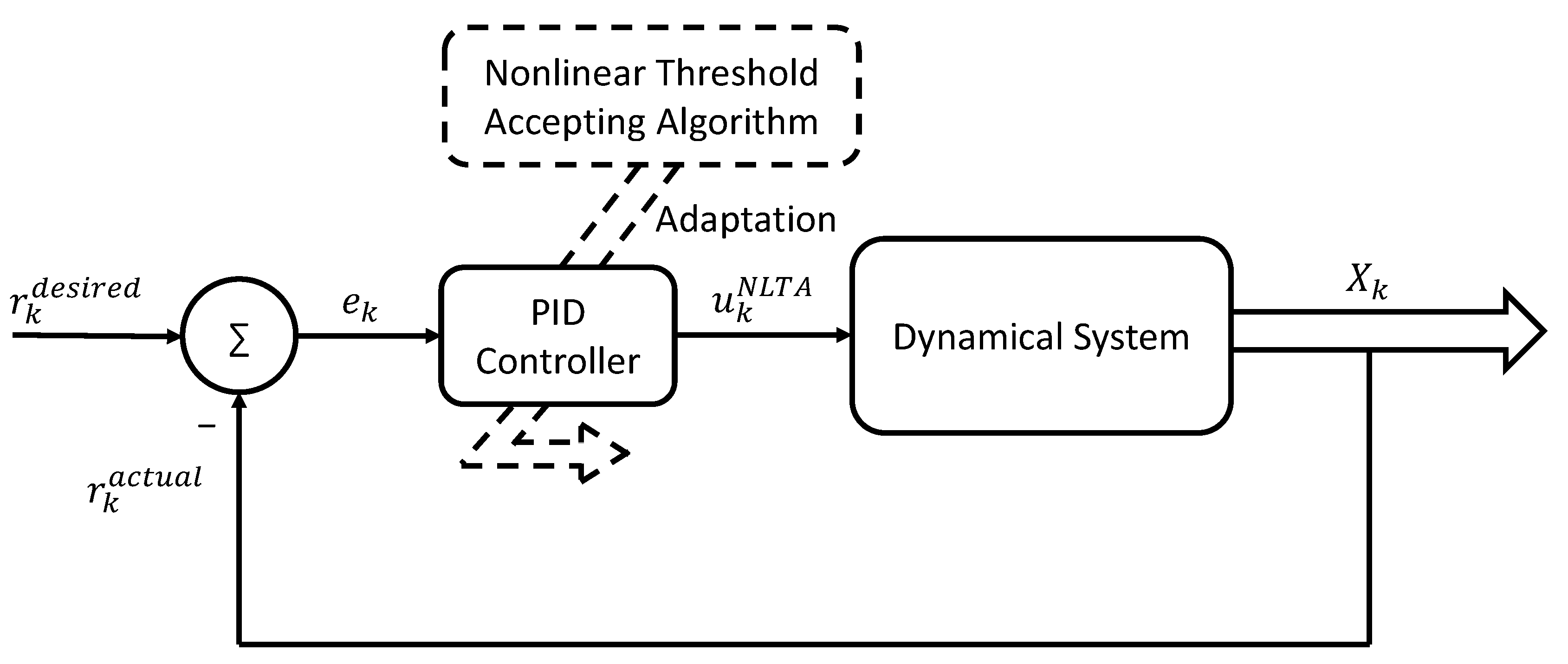
The NLTA-based controller is similar in architecture as its RL-based counterpart. However, instead of the RL, it uses the NLTA algorithm [8] to automatically tune the gains ( K p ,   K i ,   K d ) of a PID controller, as shown in Figure 3. The resulting control signal u N L T A R takes the following form:
u N L T A ( t ) = K p   e ( t ) + K i 0 t   e ( τ )   d τ + K d   d e ( t ) d t ,
where e ( t ) is the continuous-time tracking error at time t. The training of the NLTA-based controller is conducted in continuous time because NLTA is a continuous-time algorithm in nature. However, the controller is discretized into a discrete-time system after the training phase so that it can be integrated into the aggregate control structure, as shall be explained later. That way, the RL- and NLTA-based controllers can be benchmarked on a fair basis.

2.2. Cost Function Optimization

Standalone tracking processes usually overlook the optimization characteristics of the overall dynamic performance alongside the tracking process. Therefore, it is useful to adjust the dynamic tracking control signal in order to improve the overall optimization features of the underlying control system. In this work, this is achieved through an auxiliary control signal u k N N R , as shown in Figure 4. To this end, a neural network is trained using an optimized performance criteria. Unlike the tracking control schemes of Figure 2 and Figure 3, the neural network takes the full state feedback measurements X k as input in order to advise the supporting control signal u k N N , such that
u k N N = f ( X k ) ,
where f is the input-output mapping of the neural network.

2.3. Agrregate Control System

Each of the above tracking control schemes is augmented with the optimization control system of Figure 4. As such, the overall control laws of the RL- and NLTA-based controllers are defined as u T = u R L + u N N and u T = u N L T A + u N N , respectively. The dynamical system (i.e., the plant) may be defined in the time domain by either a linearized continuous- or discrete-time state-space model:
X ˙ ( t ) = A c   X ( t ) + B c   u ( t ) ,
X k + 1 = A d   X k + B d   u k ,
where the superscripts “c” and “d” denote the continuous- and discrete-time matrices, respectively. For the purpose of this study, which is conducted in the discrete-time domain, the plant model needs to be discretized if presented in the continuous-time domain. In the following, we will detail the learning paradigms of each of the control schemes.

3. Tracking Control Algorithms

3.1. RL-Based Tracking Control Algorithm

The RL process trains the tracking controller to opt for the optimal policies that minimize the tracking error. This is done through an iterative training process which continuously updates a Q-Table by penalizing or rewarding the taken actions. The table keeps track of the maximum expected future rewards for each feasible state-action pair ( E , u R L ) , where E = [ e k 3   e k 2   e k 1   e k ] T . An ϵ -greedy algorithm is applied to trade off between the exploitation and exploration of the training process. The update of the Q-Table entries follow the Q-Learning pattern, defined by [7]
Q ( E , u R L ) = Q ( E , u R L ) + α   [ R ( E , u R L ) + γ   max u + 1 R L Q ( E + 1 , u + 1 R L ) Q ( E , u R L ) ] ,
where is the agent state index, α is a learning rate, γ is a discount factor, and R ( E , u R L ) is the training reward for taking action u R L at state E . The process is detailed in Algorithm 1. Note that the accuracy of the obtained control signals u R L depends on the discretization steps of the states and the tracking errors. The finer is the resolution, the longer the learning may take.
Algorithm 1 Reinforcement Learning: Offline Computation of Q-Table
Input:
  • Minimum and maximum bounds X m i n , X m a x , u m i n R L , u m a x R L , E m i n , and E m a x of the variables X, u R L , and e, respectively.
  • Discretization steps Δ X , Δ E , and Δ u R L of the variables X, e and the control signal u R L , respectively.
  • Reinforcement learning parameters ϵ , α and γ .
Output:
   Q-Table
1:
Initialize the Q-Table randomly
2:
repeat
3:
    Update the entries of the Q-Table using (3)
4:
until A convergence criterion is met
5:
return Q-Table

3.2. NLTA-Based Tracking Control Algorithm

With the NLTA-Based Tracking method, a PID controller is applied where the PID gains are tuned using an NLTA algorithm [8]. The NLTA technique adopts the concept of a low-pass filter, whose transfer function is H ( s ) = 1 / ( 1 + s / ω 0 ) for some nominal frequency ω 0 . In particular, it bases its heuristics on the magnitude of the transfer function in the frequency domain,
H ( j ω ) = 1 / 1 + ( ω / ω 0 ) 2   ,
for some frequency ω . The magnitude function controls the convergence speed of the search process within the domains of the optimized variables. The NLTA algorithm optimizes the control gains by minimizing a tracking error-based objective cost function. In this work, the objective function is chosen to be in the form of an Integrated Squared Error (ISE), defined as
I S E = 0 t e 2 ( τ ) τ ,
with e ( τ ) being the tracking error at continuous time τ . Full details of how the NLTA is applied to optimize the gains of the PID controller are provided in Algorithm 2.
Algorithm 2 NLTA: Offline Tuning of the PID Gains
Input:
    ( K p m i n , K p m a x ) : Search range of K p .
    ( K i m i n , K i m a x ) : Search range of K i .
    ( K d m i n , K d m a x ) : Search range of K d .
    ω 0 > 0 : a nominal frequency for the low-pass filter.
    Δ ω > 0 : a frequency discount value.
    ω 1 > 0 : an initial value for ω .
   N_ITERATIONS: number of iterations per episode.
   N_EPISODES: number of episodes.
Output:
   Optimized PID gains ( K p , K i , K d ) .
1:
for  p = 1 to N_EPISODES do            ▹ Beginning of an episode
2:
    Randomly initialize the PID gains K p , K i , K d , to some stable values▹ Stability may be verified by simulating the system in Figure 3
3:
    Simulate the system in Figure 3 and calculate the ISE using (5)
4:
    ISE0 ← ISE
5:
    Smallest_ISE_p ← ISE       ▹ Smallest ISE in the episode
6:
     ω ω 1
7:
    for i = 1 to N_ITERATIONS do   ▹ Beginning of an iteration within an episode
8:
        Randomly select one PID gain candidate K p , K i or K d from its respective range
9:
        Simulate the system in Figure 3 with the PID gain candidate selected in the previous step (line 8), and calculate the ISE using (5)
10:
        ISEV ← ISE
11:
        if ISEV ISE 0 1  or ISEV ISE 0 1 H ( j ω ) then▹ The second condition allows for exploration to avoid local minima
12:
           Replace the PID gain with its candidate value   ▹ The one selected in line 8
13:
           Smallest_ISE_p ← ISEV
14:
           if ( ω Δ ω ) > 0 then
15:
                ω ω Δ ω      ▹ To control the convergence speed of the search process
16:
           end if
17:
        end if
18:
    end for
19:
     triplet ( p ) ( K p , K i , K d )         ▹ Optimized PID gains for episode p
20:
    Smallest_ISE ( p ) Smallest_ISE_p
21:
end for
22:
q arg min p Smallest _ ISE ( p )
23:
return  triplet ( q )

4. Neural Network Optimization Algorithm

A nonlinear state feedback control law u N N is developed to optimize the dynamic performance of the control scheme. It is added to the tracking control effort to form the aggregate control signal. Although the Q-Table in its simplest form can be used to control the dynamic system, it results in non-smooth discrete actions, and consequently an undesired scattered dynamic performance [53]. Therefore, the added neural network trained using this Q-Table is able to generate a continuous (non-discrete) control signal which can smooth out the system’s behavior.
To this end, two feedforward multi-layer perceptrons are trained offline for comparison purpose. Only one of them is eventually integrated in the closed-loop control system to generate an optimized value of u N N , as shall be detailed later. The training data for each neural network is prepared using a separate Q-Table with a similar structure to the one employed in the RL-based tracking controller, except that this time the full state vector is considered, instead of the tracking error combination.
The reason behind trying two neural networks is the ability to test and compare the following two objective cost functions:
F 1 ( k ) = 1 2   ( X k T   S   X k + X k + 1 T   S   X k + 1 ) + Z   ( u k N N 1 ) 2 ,
F 2 ( k ) = X k + 1 T   S   X k + 1 + Z   ( u k N N 2 ) 2 ,
where S R n × n and Z R are weighting factors reflecting the designer’s preference of how the state and the control effort are prioritized. Notice how the second performance index F 2 gives no importance to the current state, unlike F 1 . Instead, it is more driven by the future states. In the following, we will denote the neural networks trained using objective functions F 1 and F 2 by NN 1 and NN 2 , respectively; while their outputs are denoted by u N N 1 and u N N 2 .
It is worth mentioning that the cost function can also include other terms that may be of interest to the design. For instance, it can include terms related to the transient response of the system, such as the overshoot, settling time, rise time, etc. This is an appealing feature of the proposed architecture as it gives the flexibility of optimizing the terms of choice without increasing the controller’s complexity.
The training samples are arranged in two steps. The first associates the states to all possible control actions; while the second applies an optimization criteria to decide on the control action to be applied at any given state [53]. The complete training process of the neural networks is presented in Algorithm 3.
It is worth mentioning that, unlike the RL algorithm, the discretization steps Δ X j , j = 1 , , n , and Δ u N N for the measured states and the control signals, respectively, can be refined as needed without running into massive calculation overhead [53]. This is because the optimization process associated with each state X j follows a different optimization and approximation procedure. It is accomplished in one episode, unlike the RL approach which employs successive search episodes, as explained earlier.
Algorithm 3 Neural Network: Offline Energy Optimization Scheme
Input:
   Minimum and maximum bounds X j m i n , X j m a x of every state X j X , j = 1 , 2 , , n , and its discretization step Δ X j .
   Minimum and maximum bounds u m i n N N and u m a x N N of u N N , and its discretization step Δ u N N .
Output:
   Two trained neural networks, NN 1 and NN 2
1:
   Discretize the action space [ u m i n N N , u m a x N N ] into N u discrete actions: [ u 1 N N , u 2 N N , , u N u N N ] .
2:
    Discretize the state space into a single row of N X entries: [ X 1 m i n , X 1 m i n + Δ X 1 , X 1 m i n + 2 Δ X 1 , , X 1 m a x , X 2 m i n , X 2 m i n + Δ X 2 , X 2 m i n + 2 Δ X 2 , , X 2 m a x , , X n m i n , X n m i n + Δ X n , X n m i n + 2 Δ X n , , X n m a x ] .
3:
Create Q-Tables Q 1 ( 1 N u , 1 N X ) and Q 2 ( 1 N u , 1 N X ) , whose rows and columns correspond to the possible discrete actions and states formed in lines 1 and 2, respectively.
4:
Populate Q 1 and Q 2 using cost functions (6a) and (6b), respectively.
5:
Create and initialize two feedforward multi-layer perceptrons, NN 1 and NN 2 , with n inputs (corresponding to samples of states X 1 , X 2 , , X n ) and one output (corresponding to the action u).
6:
Train NN 1 and NN 2 using the data in Q 1 and Q 2 , respectively.
7:
return  NN 1 and NN 2

5. Aggregate Control Scheme

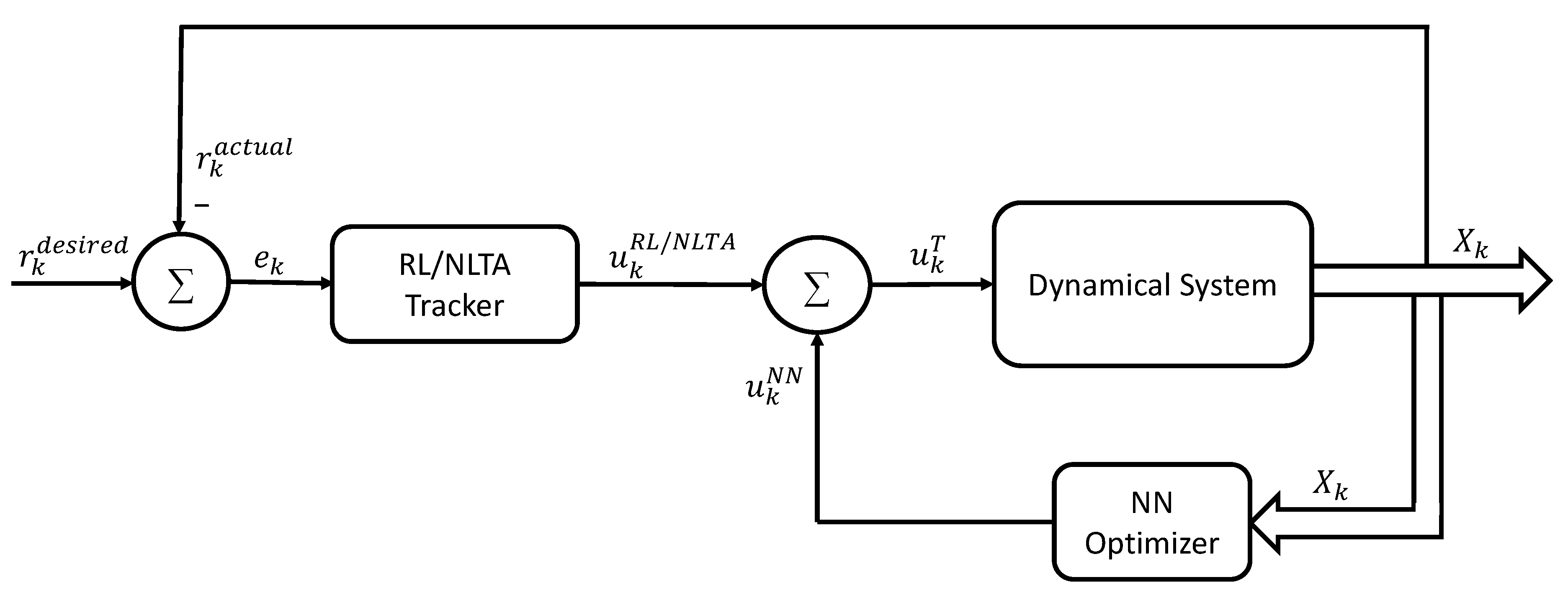
After the offline training of the RL- and the NLTA-based trackers along with the NN optimizer, they are integrated in two feedback systems of the same architecture, as shown in Figure 5. The first system uses the RL-based tracker u R L while the second system employs the NLTA-based tracker u N L T A . One of the goals of this work is to compare the performances of both systems. The aggregate control signal u k T applied to the dynamic system under consideration is either u k T = u k R L + u k N N or u k T = u k N L T A + u k N N , depending on the type of tracking controller used. In an abuse of notation, the following notation is adopted in the rest of the paper: u k T = u k R L / N L T A + u k N N . Note that u k N N is either u k N N 1 or u k N N 2 , depending on the NN optimizer used.
The two systems operate in discrete time. To adapt the NLTA-based tracker to this architecture, it needed to be discretized, since it is a continuous-time controller in nature. In other words, we needed to discretize the continuous-time PID controller whose gains were optimized using the NLTA algorithm.
The transfer function of a discrete-time PID controller in the z-domain is
u N L T A ( z ) e ( z ) = K p + K i   ·   T s   ·   z z 1 + K d T s   ·   z 1 z ,
with T s being the sampling period. This yields
u N L T A ( z )   ( 1 z 1 ) = K p   ( 1 z 1 )   e ( z ) + K i   ·   T s   ·   e ( z ) + K d T s   ( 1 2 z 1 + z 2 )   e ( z ) .
Converting to a difference equation leads to the following discrete-time control expression:
u k N L T A = u k 1 N L T A + K p   ( e k e k 1 ) + K i   ·   T s   ·   e k + K d T s   ( e k 2 e k 1 + e k 2 ) .
The proposed machine learning processes rely on heuristic tools and neural network approximations. Once the offline training phases are complete, the resulting units are applied in the closed-loop aggregate structure. The NLTA relies on a low pass filter-like accepting function to search for the best feasible combination of control gains. On another side, the reinforcement learning maximizes a cumulative reward in order to transit from one state to another while converging to an equilibrium in the process of minimizing the tracking error.

6. Simulation Results and Analysis

6.1. Simulation Setup

The proposed control architecture is applied to control the navigation of an autonomous flexible wing aircraft. This type of aircraft is described as a two-body system which is composed of a wing and a pilot/fuselage connected by a hang strap [54]. In a manned system, the pilot controls the aircraft by pushing, pulling, and rolling the control-bar which adjusts the pilot’s center relative to that of the wing [55]. The unmanned control process of flexible wing aircraft possesses many challenges. This is mainly because the system is extremely difficult to model due to its continuously varying aerodynamics [54,55,56].
The motion of an unmanned flexible wing aircraft can be decoupled into longitudinal and lateral motion frames. Herein, only the lateral motion control is tackled to validate the performance of the proposed tracking schemes. A vector of measurable states X = [ v   ϕ ˙   φ ˙   ϕ   φ ] T is considered, where v, ϕ and φ are the lateral velocity, roll attitude, and yaw attitude, respectively.
The aircraft is required to follow a desired rolling maneuver (i.e., r k d e s i r e d ) and to undergo continuous opposite banking turns as follows:
r k d e s i r e d = ϕ k d e s i r e d = 15 π 180   sin ( 4   π   k / T )   rad ,
with the following initial conditions: X 0 = [ 10   m / s 0.5   rad / s 0.5   rad / s 0 0 ] T ,   u 0 R L = u 0 N L T A = u 0 N N = 0 , where T is the total number of simulation iterations. Note that T = T d / T s , with T d = 200   s and T s = 0.01   s being the total duration of the simulation and the sampling time, respectively.
The reward function R is determined by a scalar convex cost criteria δ k = e k 2 + 0.9   e k 1 2 + 0.8   e k 2 2 + 0.7   e k 3 2 , such that
R = 100   ( 1 + e 50   ( δ k δ k + 1 ) ) ,   if   δ k + 1 < δ k 10 5 ,   if   δ k + 1 = δ k = 0 10 5 ,   otherwise .
This function assigns a positive reward if the dynamic cost δ k + 1 is less than δ k , where the highest reward is achieved at equilibrium.
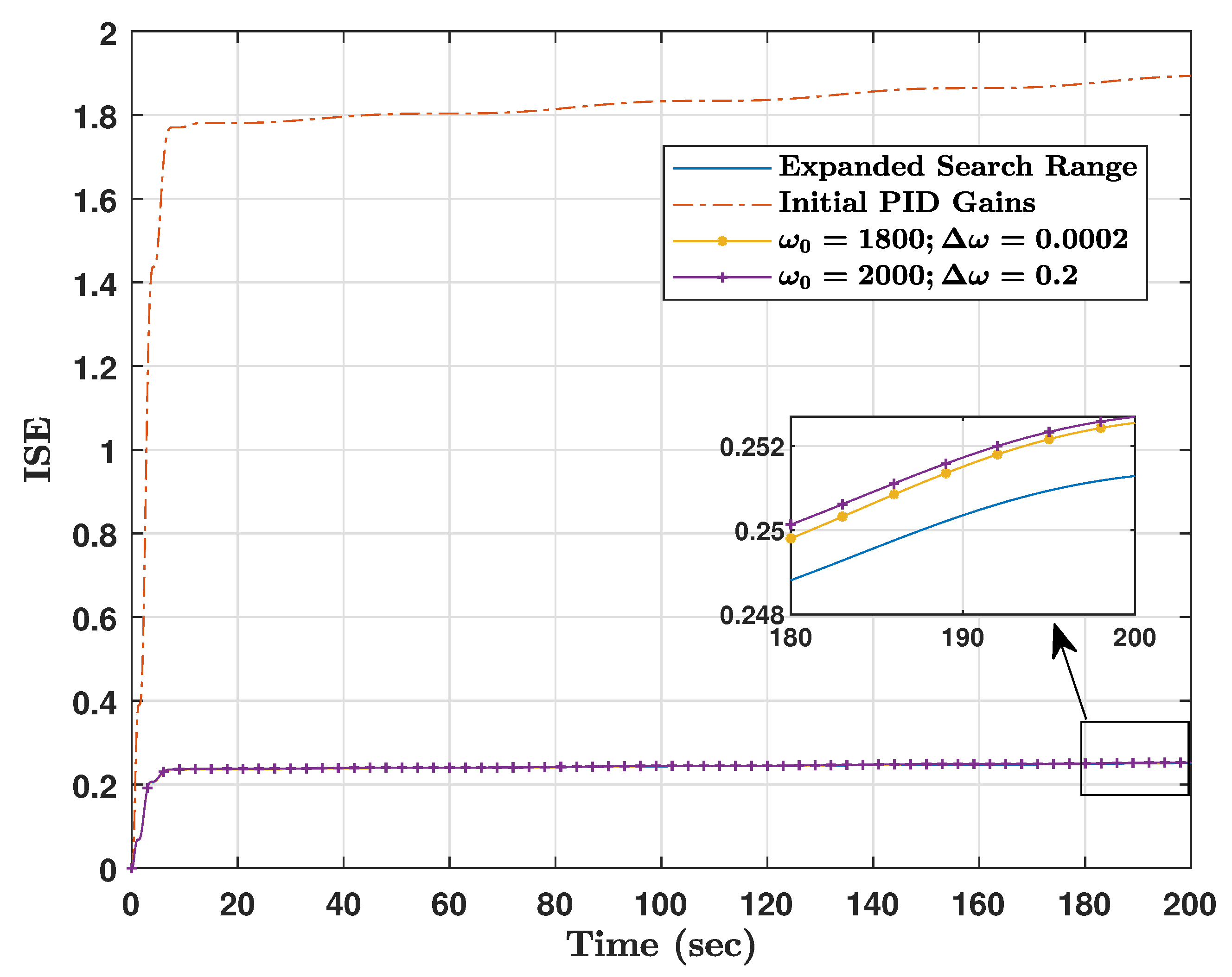
Although this is a model-free control architectural heuristic, it does depend on a priori known subset of a stable region for the gains to be optimized so that it is explored as a search space by the optimization algorithms. In general, this region can be obtained through an empirical study or/and using some already known facts about the system whenever available. For instance, with PID control gains, we already know that they ought to be positive. In addition, in this study, the search range of the PID gains is selected around an initial value ( K p = 9.9345 , K i = 4.6778 , K d = 3.5585 ) determined by Matlab’s PID Tuner so as to minimize the settling time. This tool can search for control gains that compromise between having larger closed-loop bandwidth (i.e., faster response) and having enough gain and phase margins to tackle the robustness of the tuning outcome. The NLTA parameter Δ ω should be selected small relative to the resonance frequency ω 0 in order to control the speed of the search process. The NLTA algorithm parameters and the resultant optimized PID gains are listed in Table 1 and Table 2. To show the effect of some parameters on the NLTA algorithm, the control system is simulated using the PID gains obtained by the NLTA algorithm executed with different parameter values. The ISE of these runs is plotted in Figure 6. It is clear that running the controller with the PID gains optimized by the NLTA algorithm leads to a far better ISE than with the initial PID gains.
In Q-Learning, the states and the control actions are discretized within their feasible limits where the discretization steps decide and control the overall computational time taken in learning process. In this work, the learning parameter α is set to 0.5 in order to trade-off between the previous knowledge and the new reward or learning experience. The exploration rate is set according to an ϵ -greedy algorithm to avoid falling in local maxima. The other learning parameter values are taken as ϵ = 0.9 and γ = 0.9 . The rest of the parameters are listed in Table 3. Figure 7 shows the ISE plots corresponding to RL-optimized PID gains obtained using different RL learning parameters. The results justify the parameter choices specified in Table 3.
To assess the performance of cost functions (6a) and (6b), a neural network optimizer is assigned to each of them; namely NN 1 and NN 2 , respectively. The structure and training parameters of the neural network optimizers are summarized in Table 4. The weighting matrices S and Z are selected as to weigh the importance of the different dynamic signals in each of the cost functions. They are set to
S = [ 0.0025 0 0 0 0 0 0.25 0 0 0 0 0 0.25 0 0 0 0 0 5.1653 0 0 0 0 0 5.1653 ] ,   Z = 0.0517 .
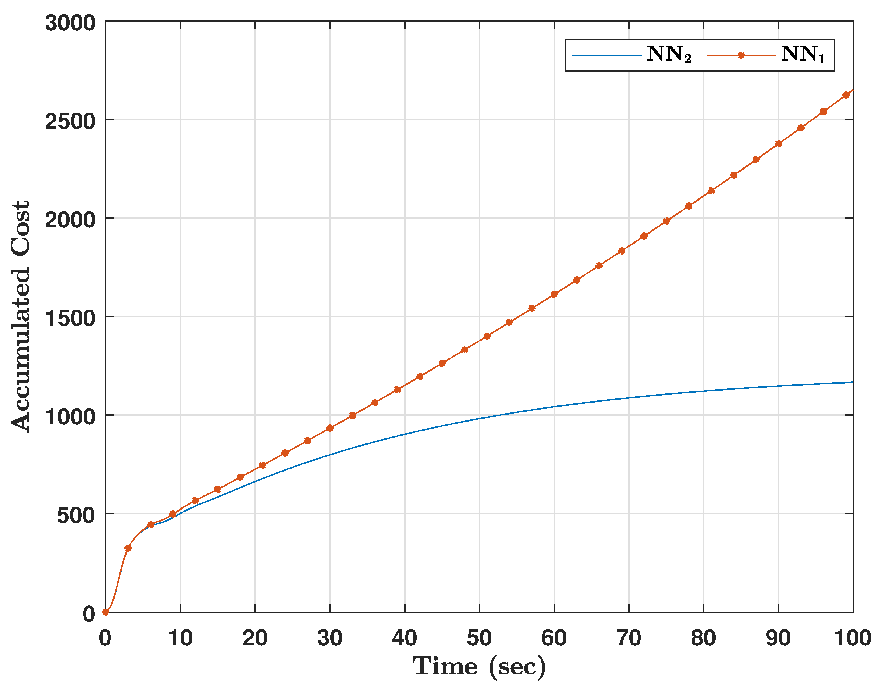
At first, both neural network optimizers are compared based on their accumulated cost k = 1 T F i ( k ) , i { 1 , 2 } , to decide on the one to adopt in the optimization loop of the aggregate control system (Figure 5). The results are illustrated in Figure 8. They show that NN 2 yields a lower cumulative dynamic cost compared to that of NN 1 . As such, NN 2 is chosen as the control optimizer in the subsequent simulations. To demonstrate the neural network’s sensitivity to some of its parameters and the appropriateness of the values adopted in Table 4, the control system is run with NN 2 after it is trained with different number of hidden neurons (NOH) and discretization steps (NOS) of the state and action spaces. The latter is specified as 20 in Table 4. The results are displayed in Figure 9. The figure reveals the importance of having finer NOS. However, too small values may make the learning time excessively long. The number of hidden neurons is chosen to be just enough to capture the system’s complexity without risking to over train the network.
Herein, we opted to focus more on the structure of the AI mechanisms after testing sufficient sets of initial learning environments and choosing the best combinations that compromise among our objectives. In the following, we will refer to the RL- and NLTA-based trackers with and without the neural network optimizer as RL, RL+NN, NLTA, and NLTA+NN.

6.2. Performance Analysis

Three simulation scenarios are considered. The first adopts the dynamic model of the aircraft at nominal trim speed and flight condition. In the second scenario, a sudden variation in the dynamic model is applied at time t s = 20   s (corresponding to k s = t s / T s = 2000 ). It aims at assessing the controller’s performance in the face of a sudden drop in the aircraft’s payload, for example. Finally, a more aggressive simulation scenario is considered, where the dynamics of the aircraft are allowed to vary around their nominal values ( A 1 d and B 1 d ) at each evolution step k. The variation of each state (shown in Figure 10) is drawn from a normal distribution of zero mean and a variance of 0.5 . The dynamics of the three scenarios are summarized in Table 5, where for every element ( i , j ) of matrices A k d ^ and B k d ^ , is defined as
A k d ^ ( i , j ) = ( 1 + σ A )   A 1 k d ^ ( i , j ) , B k d ^ ( i , j ) = ( 1 + σ B )   B 1 k d ^ ( i , j ) ,
where σ A , σ B N ( 0 , 0.5 ) .
The discrete-time state space matrices are adopted from [55] as
A 1 d = [ 0.9977 0.0028 0.1069 0.0971 0.0131 0.0131 0.8092 0.0677 0 0 0.0026 0.0333 0.9802 0 0 0 0.0090 0 1 0 0 0 0.0099 0 1 ] ,   B 1 d = [ 0 0.0324 0.0036 0 0 ] ,
A 2 d = [ 0.9987 0.0028 0.0940 0.1230 0.0170 0.0090 0.8112 0.0637 0.0006 0.0001 0.0031 0.0402 0.9752 0.0002 0 0 0.0090 0.0003 1 0 0 0.0002 0.0099 0 1 ] ,   B 2 d = [ 0.0002 0.0251 0.0044 0.0001 0 ] .
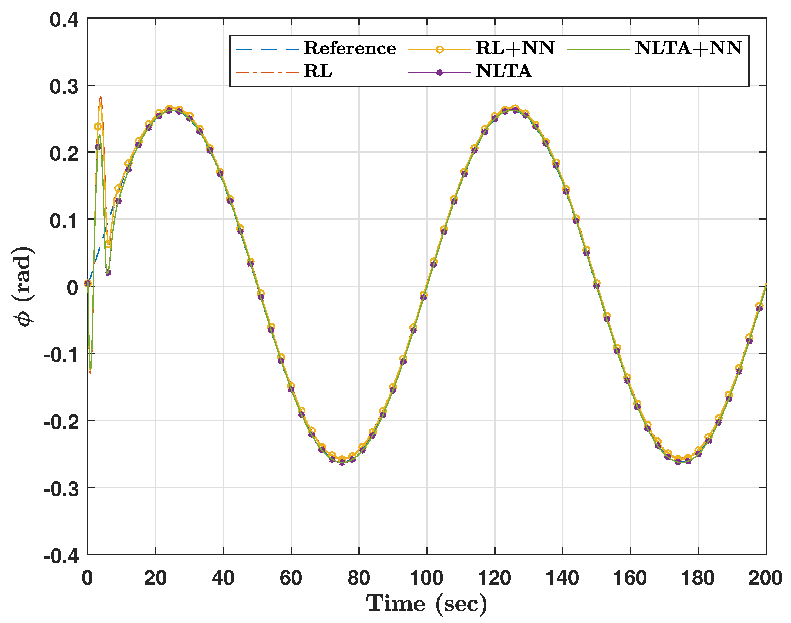
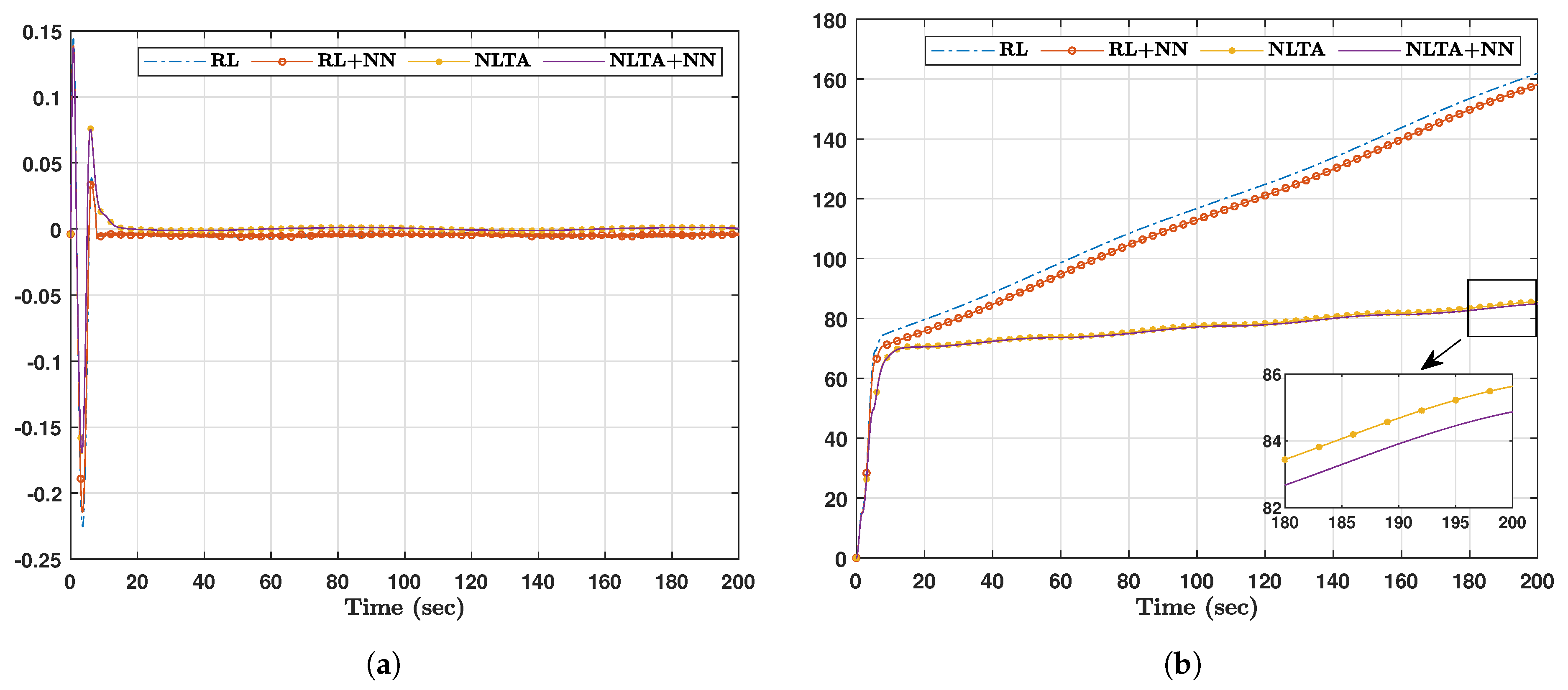
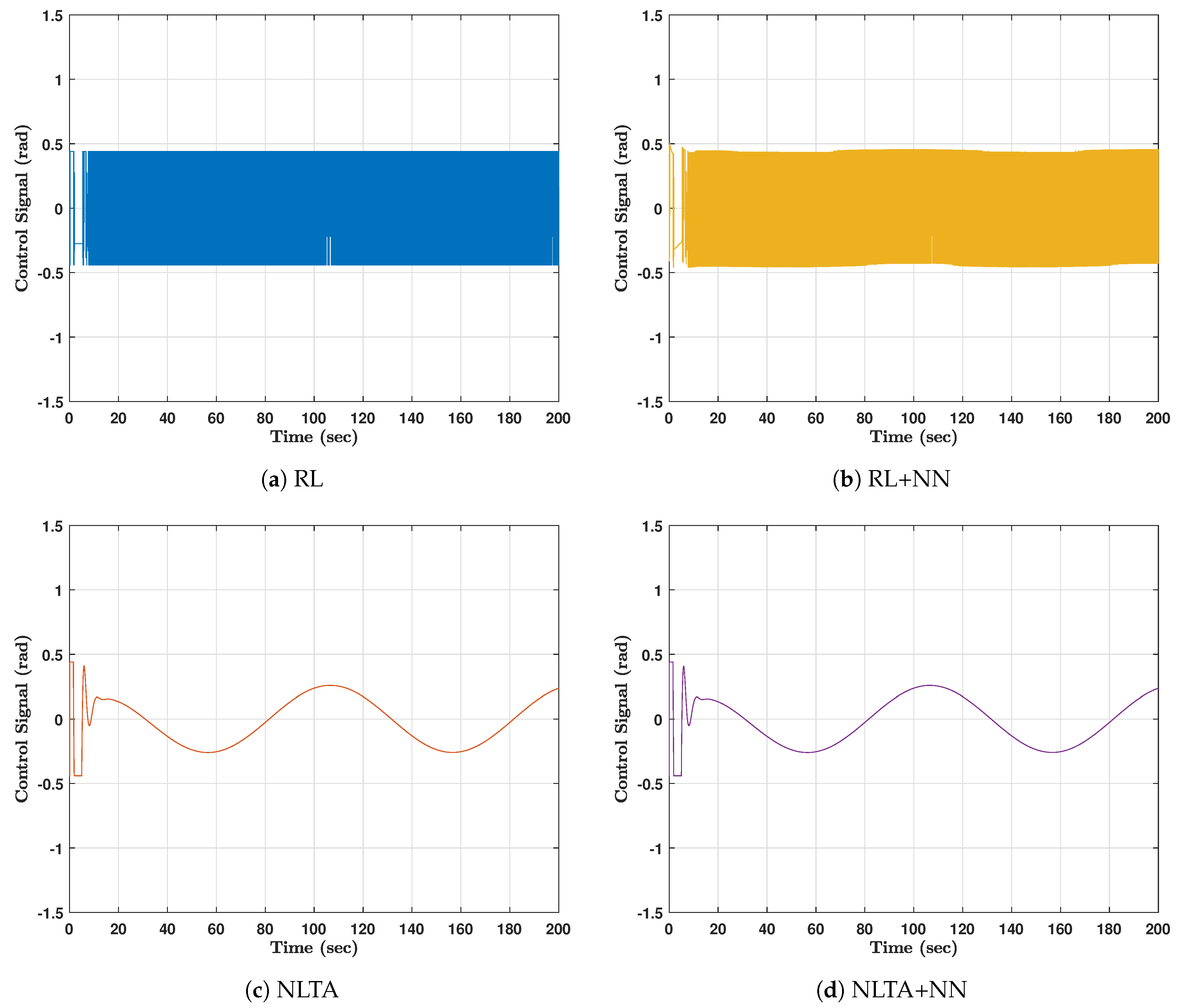
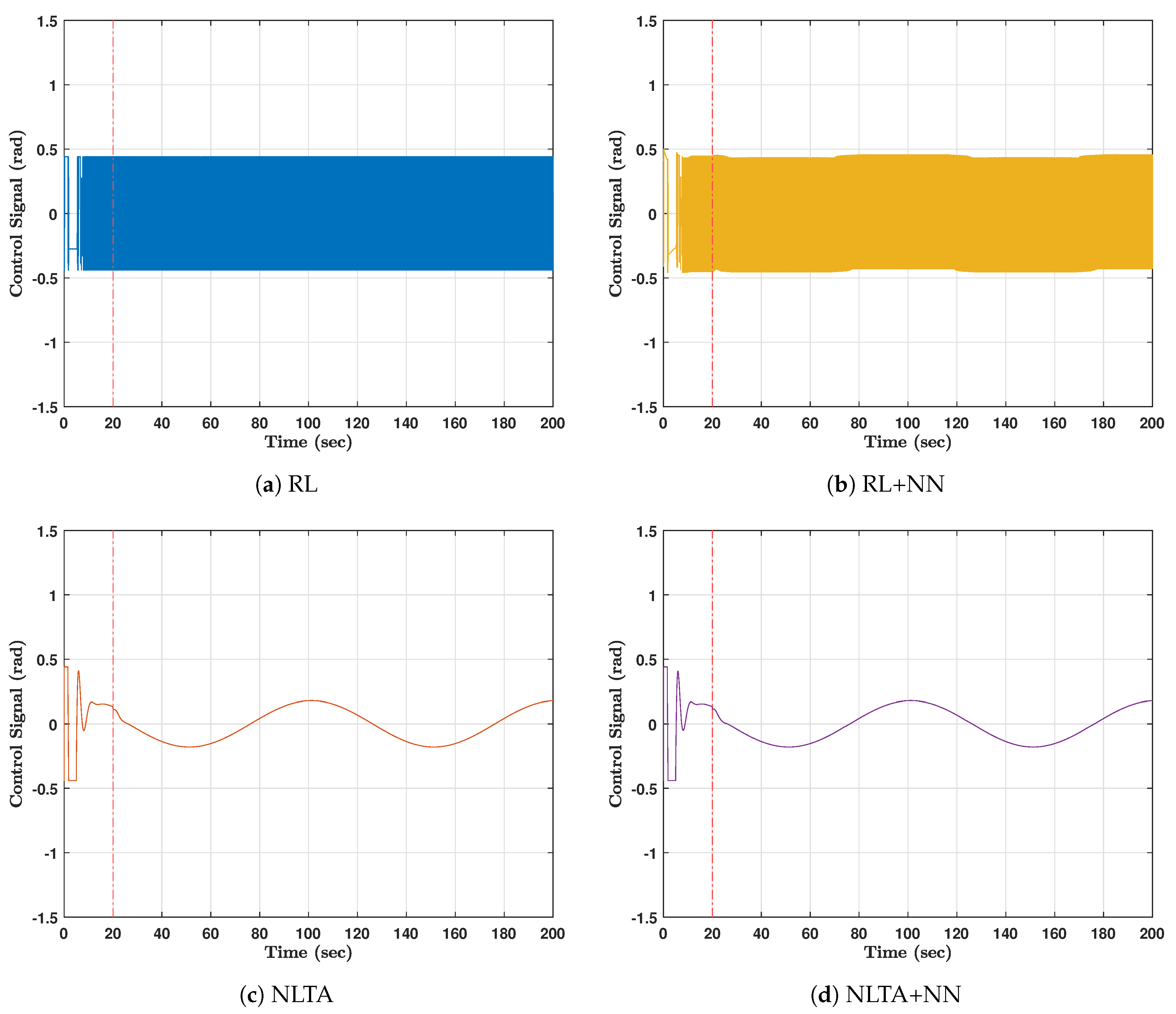
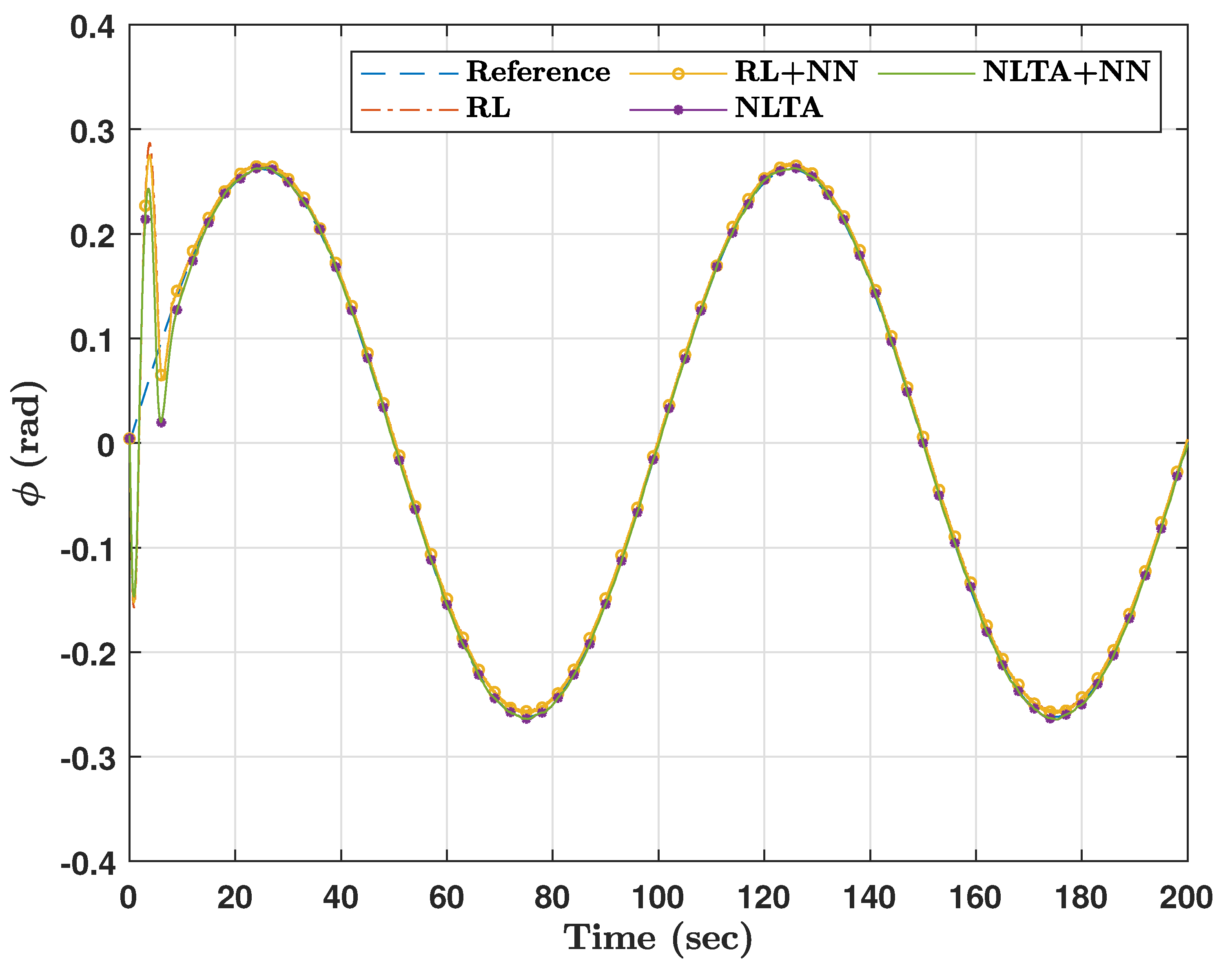
The aircraft banking simulation results of the first scenario are shown in Figure 11, Figure 12 and Figure 13. The RL- and NLTA-based trackers with and without the neural network optimizer are able to asymptotically stabilize the aircraft around the desired banking trajectory ϕ k d e s i r e d . The tracking errors and the control signals of RL and RL+NN are characterized by a chattering behavior within the envelopes [ 0.005 rad , 0 ] and [ 0.45 rad , + 0.45 rad ] , respectively. Nevertheless, the tracking errors generated NLTA and NLTA+NN are asymptotically convergent. It also worth noticing that the control signals of the latter controllers are significantly smoother than their counterparts dispatched by RL and RL+NN. Figure 12 clearly demonstrates that the neural network optimizer contributes to reducing the cumulative tracking error, however small this contribution might be. The total energy cost k = 1 T X k + 1 T   S   X k + 1 + Z   ( u k T ) 2 , of the four controllers across the three scenarios are summarized in Table 6. From this measure, we can deduce that the controllers share similar performances due to the insignificant differences in their total costs. It is interesting to notice that, the NLTA+NN variant of the controller achieved the lowest total energy cost.
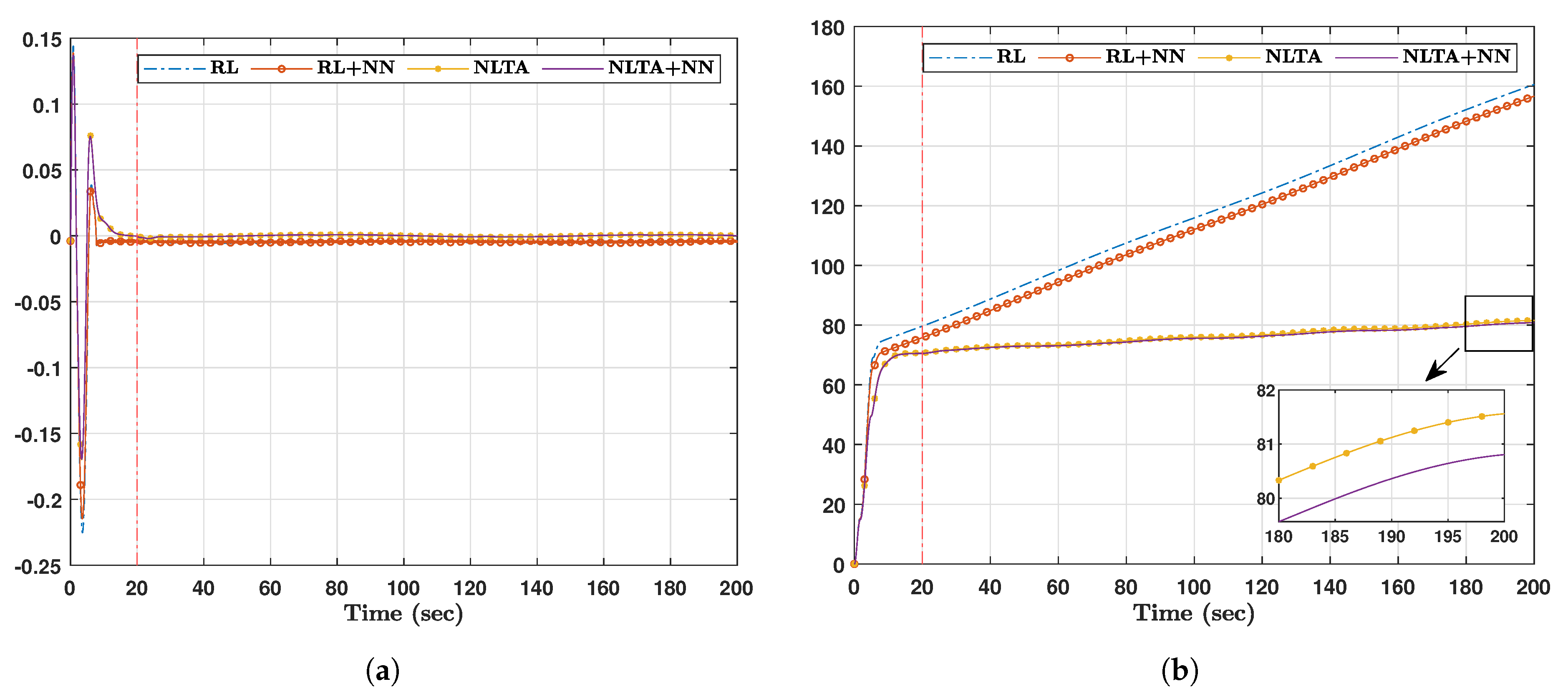
The same remarks are confirmed by the simulation of the second scenario. The results are depicted in Figure 14, Figure 15 and Figure 16. The proposed control structures initially took a few seconds to converge to the reference signal from the initial condition, as shown in Figure 14. However, once on track, it is interesting to notice that they were virtually insensitive to the abrupt change in the system dynamics at time t = 20   s . The system robustness is clearly revealed again in Figure 14 and Figure 15. The influence of the neural network optimizer in improving the performances of the standalone tracking units is demonstrated in Figure 15b and Table 6. Furthermore, the resulting control signals generated by the tracking controllers are shown in Figure 16 where the NLTA and NLTA+NN exhibited smooth behavior compared to that of RL and RL+NN.
The third scenario emulates an aggressive test case, where the dynamics are time-variant this time with an excessive disturbance term. The results are revealed in Figure 17, Figure 18, Figure 19 and Figure 20. The NLTA and NLTA+NN controllers effectively guide the aircraft towards the desired trajectory with less fluctuations than RL and RL+NN, as shown in Figure 17 and Figure 18. This is clearly illustrated by examining the roll angle rate ϕ ˙ indicator in Figure 20c. This scenario articulates the advantage of adding the neural network optimizer, as shown in Figure 18b and Table 6. It is in such a case that the difference between the trackers with and without the neural network optimizer is most significant. The generated control signals and hence the associated system states, reacting to the disturbance in the dynamics, are depicted in Figure 19 and Figure 20, respectively. The resulting control signals show instantaneous counteractions made by the tracking controllers in response to the imposed disturbance leading to the performance demonstrated in Figure 17 and Figure 20.

7. Conclusions

The article presents a synergetic integration approach of machine learning tools to provide a model-free solution for a class of tracking control problems. The proposed family of controllers solve the underlying problem using two control loops: one for tracking and one to optimize an overall performance measure. The controllers are tested on a navigation mechanism of a flexible wing aircraft with uncertain/varying dynamics. After an offline training process, they demonstrated a high ability to simultaneously minimize the tracking error and the total energy cost in different test cases of varying complexities. They also succeeded to maintain the system’s stability in the face of excessive disturbances. The neural network optimizer proved to well complement the trackers to better annihilate the cumulative tracking error as well as further reduce the total energy cost. Although the four controllers showed a comparable performance in terms of cumulative cost, NLTA and NLTA+NN tend to generate smoother control signals and asymptotically convergent tracking errors.

Author Contributions

All authors have made great contributions to the work. Conceptualization, N.W., M.A., W.G. and N.N.; Methodology, N.W., M.A., W.G., and N.N.; Investigation, N.W.; Validation, M.A. and W.G.; Writing-Review & Editing, N.W., M.A., W.G. and N.N. All authors have read and agreed to the published version of the manuscript.

Funding

This research was partially funded by Ontario Centres of Excellence (OCE) and the Natural Sciences and Engineering Research Council of Canada (NSERC).

Conflicts of Interest

The authors declare no conflict of interest. The funding sponsors had no role in the design of the study; in the collection, analyses, or interpretation of data; in the writing of the manuscript, and in the decision to publish the results.

Abbreviations

The following abbreviations are used in this manuscript:
Variables
vLinear side velocity
ϕ , φ Roll and yaw angles in the wing’s frame of motion
Abbreviations
RLReinforcement Learning
NLTANonlinear Threshold Accepting
NNNeural Network
NPNon-deterministic Polynomial-time
PIDProportional-Integral-Derivative

References

  1. Ernst, D.; Glavic, M.; Wehenkel, L. Power systems stability control: Reinforcement learning framework. IEEE Trans. Power Syst. 2004, 19, 427–435. [Google Scholar] [CrossRef] [Green Version]
  2. Luy, N.T. Reinforecement learning-based optimal tracking control for wheeled mobile robot. In Proceedings of the 2012 IEEE International Conference on Cyber Technology in Automation, Control, and Intelligent Systems (CYBER), Bangkok, Thailand, 27–31 May 2012; pp. 371–376. [Google Scholar]
  3. Figueroa, R.; Faust, A.; Cruz, P.; Tapia, L.; Fierro, R. Reinforcement learning for balancing a flying inverted pendulum. In Proceedings of the 11th World Congress on Intelligent Control and Automation, Shenyang, China, 29 June–4 July 2014; pp. 1787–1793. [Google Scholar]
  4. Peters, J.; Vijayakumar, S.; Schaal, S. Reinforcement learning for humanoid robotics. In Proceedings of the Third IEEE-RAS International Conference on Humanoid Robots, Karlsruhe, Germany, 29–30 September 2003. [Google Scholar]
  5. Côté, D. Using machine learning in communication networks. J. Opt. Commun. Netw. 2018, 10, D100–D109. [Google Scholar] [CrossRef]
  6. Jordan, M.I.; Mitchell, T.M. Machine learning: Trends, perspectives, and prospects. Science 2015, 349, 255–260. [Google Scholar] [CrossRef]
  7. Sutton, R.S.; Barto, A.G. Reinforcement Learning: An Introduction, 2nd ed.; MIT Press: Cambridge, MA, USA, 1998. [Google Scholar]
  8. Nahas, N.; Abouheaf, M.; Sharaf, A.M.; Gueaieb, W. A Self-Adjusting Adaptive AVR-LFC Scheme for Synchronous Generators. IEEE Trans. Power Syst. 2019, 34, 5073–5075. [Google Scholar] [CrossRef]
  9. Kober, J.; Bagnell, J.A.; Peters, J. Reinforcement learning in robotics: A survey. Int. J. Robot. Res. 2013, 32, 1238–1274. [Google Scholar] [CrossRef] [Green Version]
  10. Kiumarsi, B.; Vamvoudakis, K.G.; Modares, H.; Lewis, F.L. Optimal and Autonomous Control Using Reinforcement Learning: A Survey. IEEE Trans. Neural Netw. Learn. Syst. 2018, 29, 2042–2062. [Google Scholar] [CrossRef]
  11. Watkins, C.J.C.H. Learning from Delayed Rewards. Ph.D. Thesis, King’s College, Cambridge, UK, May 1989. [Google Scholar]
  12. Abouheaf, M.I.; Lewis, F.L. Multi-agent differential graphical games: Nash online adaptive learning solutions. In Proceedings of the 52nd IEEE Conference on Decision and Control, Florence, Italy, 10–13 December 2013; pp. 5803–5809. [Google Scholar] [CrossRef]
  13. Abouheaf, M.I.; Lewis, F.L.; Mahmoud, M.S. Model-free adaptive learning solutions for discrete-time dynamic graphical games. In Proceedings of the 53rd IEEE Conference on Decision and Control, Los Angeles, CA, USA, 15–17 December 2014; pp. 3578–3583. [Google Scholar] [CrossRef]
  14. Abouheaf, M.I.; Lewis, F.L.; Mahmoud, M.S. Differential graphical games: Policy iteration solutions and coupled Riccati formulation. In Proceedings of the 2014 European Control Conference (ECC), Strasbourg, France, 24–27 June 2014; pp. 1594–1599. [Google Scholar]
  15. Abouheaf, M.; Lewis, F.; Vamvoudakis, K.; Haesaert, S.; Babuska, R. Multi-Agent Discrete-Time Graphical Games And Reinforcement Learning Solutions. Automatica 2014, 50, 3038–3053. [Google Scholar] [CrossRef] [Green Version]
  16. Abouheaf, M.I.; Lewis, F.L. Dynamic Graphical Games: Online Adaptive Learning Solutions Using Approximate Dynamic Programming. In Frontiers of Intelligent Control and Information Processing; World Scientific: Singapore, 2015; pp. 1–48. [Google Scholar]
  17. Abouheaf, M.I.; Haesaert, S.; Lee, W.; Lewis, F.L. Q-Learning with Eligibility Traces to solve Non-Convex economic dispatch problems. Int. J. Electr. Sci. Eng. 2012, 7, 1390–1396. [Google Scholar]
  18. Slotine, J.J.; Sastry, S.S. Tracking control of non-linear systems using sliding surfaces, with application to robot manipulators. Int. J. Control 1983, 38, 465–492. [Google Scholar] [CrossRef] [Green Version]
  19. Jiang, Z.P.; Nijmeijer, H. Tracking control of mobile robots: A case study in backstepping. Automatica 1997, 33, 1393–1399. [Google Scholar] [CrossRef] [Green Version]
  20. Chen, B.; Liu, X.; Tong, S. Adaptive fuzzy output tracking control of MIMO nonlinear uncertain systems. IEEE Trans. Fuzzy Syst. 2007, 15, 287–300. [Google Scholar] [CrossRef]
  21. Zhang, H.; Wei, Q.; Luo, Y. A novel infinite-time optimal tracking control scheme for a class of discrete-time nonlinear systems via the greedy HDP iteration algorithm. IEEE Trans. Syst. Man Cybern. Part B Cybern. 2008, 38, 937–942. [Google Scholar] [CrossRef] [PubMed]
  22. Cheah, C.C.; Liu, C.; Slotine, J.J.E. Adaptive tracking control for robots with unknown kinematic and dynamic properties. Int. J. Robot. Res. 2006, 25, 283–296. [Google Scholar] [CrossRef]
  23. Repoulias, F.; Papadopoulos, E. Planar trajectory planning and tracking control design for underactuated AUVs. Ocean Eng. 2007, 34, 1650–1667. [Google Scholar] [CrossRef]
  24. O’Dwyer, A. Handbook of PI and PID Controller Tuning Rules; Imperial College Press: London, UK, 2009. [Google Scholar]
  25. Singh, S.; Mitra, R. Comparative analysis of robustness of optimally offline tuned PID controller and Fuzzy supervised PID controller. In Proceedings of the 2014 Recent Advances in Engineering and Computational Sciences (RAECS), Chandigarh, India, 6–8 March 2014; pp. 1–6. [Google Scholar] [CrossRef]
  26. Fu, H.; Chen, X.; Wang, W.; Wu, M. MRAC for unknown discrete-time nonlinear systems based on supervised neural dynamic programming. Neurocomputing 2020, 384, 130–141. [Google Scholar] [CrossRef]
  27. Radac, M.B.; Lala, T. Learning Output Reference Model Tracking for Higher-Order Nonlinear Systems with Unknown Dynamics. Algorithms 2019, 12, 121. [Google Scholar] [CrossRef] [Green Version]
  28. Tang, D.; Chen, L.; Tian, Z.F.; Hu, E. Modified value-function-approximation for synchronous policy iteration with single-critic configuration for nonlinear optimal control. Int. J. Control 2019, 1–13. [Google Scholar] [CrossRef]
  29. Mu, C.; Ni, Z.; Sun, C.; He, H. Data-Driven Tracking Control With Adaptive Dynamic Programming for a Class of Continuous-Time Nonlinear Systems. IEEE Trans. Cybern. 2017, 47, 1460–1470. [Google Scholar] [CrossRef]
  30. Mu, C.; Zhang, Y. Learning-Based Robust Tracking Control of Quadrotor with Time-Varying and Coupling Uncertainties. IEEE Trans. Neural Netw. Learn. Syst. 2020, 31, 259–273. [Google Scholar] [CrossRef]
  31. Nahas, N.; Nourelfath, M. Nonlinear threshold accepting meta-heuristic for combinatorial optimisation problems. Int. J. Metaheuristics 2014, 3, 265–290. [Google Scholar] [CrossRef]
  32. Nahas, N.; Darghouth, M.N.; Kara, A.Q.; Nourelfath, M. Non-linear threshold algorithm based solution for the redundancy allocation problem considering multiple redundancy strategies. J. Qual. Maint. Eng. 2019, 25, 397–411. [Google Scholar] [CrossRef]
  33. Nahas, N.; Darghouth, M.N.; Abouheaf, M. A non-linear-threshold-accepting function based algorithm for the solution of economic dispatch problem. RAIRO Oper. Res. 2020, 54. [Google Scholar] [CrossRef] [Green Version]
  34. Jain, A.K.; Mao, J.; Mohiuddin, K.M. Artificial neural networks: A tutorial. Computer 1996, 29, 31–44. [Google Scholar] [CrossRef] [Green Version]
  35. Svozil, D.; Kvasnicka, V.; Pospichal, J. Introduction to multi-layer feed-forward neural networks. Chemom. Intell. Lab. Syst. 1997, 39, 43–62. [Google Scholar] [CrossRef]
  36. Yao, X. Evolving artificial neural networks. Proc. IEEE 1999, 87, 1423–1447. [Google Scholar]
  37. Beigzadeh, R.; Rahimi, M.; Shabanian, S.R. Developing a feed forward neural network multilayer model for prediction of binary diffusion coefficient in liquids. Fluid Phase Equilib. 2012, 331, 48–57. [Google Scholar] [CrossRef]
  38. Oczak, M.; Viazzi, S.; Ismayilova, G.; Sonoda, L.T.; Roulston, N.; Fels, M.; Bahr, C.; Hartung, J.; Guarino, M.; Berckmans, D.; et al. Classification of aggressive behaviour in pigs by activity index and multilayer feed forward neural network. Biosyst. Eng. 2014, 119, 89–97. [Google Scholar] [CrossRef]
  39. Liang, P.; Bose, N. Neural Network Fundamentals with Graphs, Algorithms and Applications; Mac Graw-Hill: Pennsylvania Plaza, NY, USA, 1996. [Google Scholar]
  40. Golomb, B.A.; Lawrence, D.T.; Sejnowski, T.J. SEXnet: A neural network identifies sex from human faces. In Advances in Neural Information Processing Systems; Touretzky, D.S., Lippmann, R., Eds.; Morgan Kaufmann: San Mateo, CA, USA, 1991; Volume 3. [Google Scholar]
  41. Rowley, H.A.; Baluja, S.; Kanade, T. Neural network-based face detection. IEEE Trans. Pattern Anal. Mach. Intell. 1998, 20, 23–38. [Google Scholar] [CrossRef]
  42. Park, D.C.; El-Sharkawi, M.; Marks, R.; Atlas, L.; Damborg, M. Electric load forecasting using an artificial neural network. IEEE Trans. Power Syst. 1991, 6, 442–449. [Google Scholar] [CrossRef] [Green Version]
  43. Chen, F.C.; Khalil, H.K. Adaptive control of nonlinear systems using neural networks. Int. J. Control 1992, 55, 1299–1317. [Google Scholar] [CrossRef]
  44. Kim, B.S.; Calise, A.J. Nonlinear flight control using neural networks. J. Guid. Control Dyn. 1997, 20, 26–33. [Google Scholar] [CrossRef]
  45. Minemoto, T.; Isokawa, T.; Nishimura, H.; Matsui, N. Feed forward neural network with random quaternionic neurons. Signal Process. 2017, 136, 59–68. [Google Scholar] [CrossRef]
  46. Hagan, M.T.; Menhaj, M.B. Training feedforward networks with the Marquardt algorithm. IEEE Trans. Neural Netw. 1994, 5, 989–993. [Google Scholar] [CrossRef]
  47. Fun, M.H.; Hagan, M.T. Levenberg-Marquardt training for modular networks. In Proceedings of the International Conference on Neural Networks (ICNN’96), Washington, DC, USA, 3–6 June 1996; pp. 468–473. [Google Scholar]
  48. Bansal, S.; Calandra, R.; Xiao, T.; Levine, S.; Tomlin, C.J. Goal-Driven Dynamics Learning via Bayesian Optimization. In Proceedings of the 2017 IEEE 56th Annual Conference on Decision and Control (CDC), Melbourne, VIC, Australia, 12–15 December 2017. [Google Scholar]
  49. Zhao, J.; Na, J.; Gao, G. Adaptive dynamic programming based robust control of nonlinear systems with unmatched uncertainties. Neurocomputing 2020, 395, 56–65. [Google Scholar] [CrossRef]
  50. Wang, N.; Pan, X. Path Following of Autonomous Underactuated Ships: A Translation–Rotation Cascade Control Approach. IEEE/ASME Trans. Mechatron. 2019, 24, 2583–2593. [Google Scholar] [CrossRef]
  51. Yao, D.; Li, H.; Lu, R.; Shi, Y. Distributed Sliding-Mode Tracking Control of Second-Order Nonlinear Multiagent Systems: An Event-Triggered Approach. IEEE Trans. Cybern. 2020, 1–11. [Google Scholar] [CrossRef] [PubMed]
  52. Lewis, F.L.; Vrabie, D.; Syrmos, V.L. Optimal Control; John Wiley & Sons: Hoboken, NJ, USA, 2012. [Google Scholar]
  53. Abouheaf, M.; Gueaieb, W. Neurofuzzy Reinforcement Learning Control Schemes for Optimized Dynamical Performance. In Proceedings of the 2019 IEEE International Symposium on Robotic and Sensors Environments (ROSE), Ottawa, ON, Canada, 17–18 June 2019; pp. 1–7. [Google Scholar]
  54. de Matteis, G. Dynamics of Hang Gliders. J. Guid. Control Dyn. 1991, 14, 1145–1152. [Google Scholar] [CrossRef]
  55. Cook, M.; Spottiswoode, M. Modelling the Flight Dynamics of the Hang Glider. Aeronaut. J. 2006, 109, I–XX. [Google Scholar] [CrossRef] [Green Version]
  56. De Matteis, G. Response of Hang Gliders to Control. Aeronaut. J. 1990, 94, 289–294. [Google Scholar] [CrossRef]
Figure 1. Agent-environment interaction.
Robotics 09 00049 g001
Figure 2. RL tracking control scheme.
Robotics 09 00049 g002
Figure 3. NLTA tracking control scheme.
Robotics 09 00049 g003
Figure 4. Neural network-based optimization control scheme.
Robotics 09 00049 g004
Figure 5. Combined tracking control scheme.
Robotics 09 00049 g005
Figure 6. ISE for different NLTA search parameters. “Expanded Search Range” refers to the PID gains obtained by running the NLTA with the parameters in Table 1. “Initial PID Gains” refers to the case where the PID gains were not tuned by the NLTA. The other two cases are related to the PID gains obtained by running the NLTA algorithm with the parameters in Table 1 except the ones specified by legend labels.
Robotics 09 00049 g006
Figure 7. ISE for different Q-learning parameters. The rest of the parameters are listed in Table 3.
Robotics 09 00049 g007
Figure 8. Accumulated cost function values for NN 1 and NN 2 .
Robotics 09 00049 g008
Figure 9. Accumulated cost function values for different NN-training parameters. The rest of the parameters are presented in Table 4.
Robotics 09 00049 g009
Figure 10. Variations in the dynamics.
Robotics 09 00049 g010
Figure 11. Roll trajectory tracking of Model 1.
Robotics 09 00049 g011
Figure 12. (a) Tracking error ( rad ) , and (b) Cumulative tracking error ( rad ) for Model 1.
Robotics 09 00049 g012
Figure 13. Control signals for Model 1.
Robotics 09 00049 g013
Figure 14. Roll trajectory tracking of Model 2.
Robotics 09 00049 g014
Figure 15. (a) Tracking error ( rad ) , and (b) Cumulative tracking error ( rad ) for Model 2.
Robotics 09 00049 g015
Figure 16. Control signals for Model 2.
Robotics 09 00049 g016
Figure 17. Roll trajectory tracking of Model 3.
Robotics 09 00049 g017
Figure 18. (a) Tracking error ( rad ) , and (b) Cumulative tracking error ( rad ) for Model 3.
Robotics 09 00049 g018
Figure 19. Control signals for Model 3.
Robotics 09 00049 g019
Figure 20. System states: (a) side velocity v ( m / s ), (b) yaw angle φ ( rad ), (c) roll angle rate ϕ ˙ ( rad / s ), and (d) yaw angle rate φ ˙ ( rad / s ) ( ϕ is omitted since it is plotted in Figure 17).
Robotics 09 00049 g020aRobotics 09 00049 g020b
Table 1. Parameters of the NLTA-based Tracker.
ParametersValues
( K p m i n , K p m a x ) (0,30)
( K i m i n , K i m a x ) (0,15)
( K d m i n , K d m a x ) (0,11)
ω 0 [ rad / s ] 2 × 10 3
Δ ω [ rad / s ] 0.0002
ω 1 [ rad / s ] 2.2 × 10 3
N_EPISODES10
N_ITERATIONS 10 5
Table 2. Optimized PID Control Gains.
K p K i K d
29.7770 12.7673 10.6736
Table 3. Parameters of the RL-based Tracker.
ParametersValues
X m i n , X m a x ± [ 20   m / s 2   rad / s 2   rad / s 0.44   rad 0.44   rad ] T
u m i n R L , u m a x R L ± 0.44   rad
E m i n , E m a x ± 0.44   rad
Δ X [ 4   m / s 0.4   rad / s 0.4   rad / s 0.055   rad 0.055   rad ] T
Δ E 0.35 rad
Δ u R L 0.055 rad
α 0.5
γ 0.9
ϵ 0.9
Table 4. Parameters of the Neural Network Optimizers.
ParametersValues
X m i n , X m a x ± [ 20   m / s 2   rad / s 2   rad / s 0.44   rad 0.44   rad ] T
u m i n N N , u m a x N N ± 0.44   rad
Δ X ( X m a x X m i n ) / 20
Δ u N N ( u m a x N N u m i n N N ) / 20
Number of hidden layers1
Number of hidden neurons13
Size of data set 4,084,000 samples
Training date set 70 %
Validation date set 15 %
Testing data set 15 %
Learning algorithmLevenberg-Marquardt
Table 5. Simulation Scenarios.
Model 1Model 2Model 3
X k + 1 = A 1 d   X k + B 1 d   u k X k + 1 = A 1 d   X k + B 1 d   u k ,   k k s
X k + 1 = A 2 d   X k + B 2 d   u k ,   k > k s
X k + 1 = A k d ^   X k + B k d ^   u k
Table 6. Total Energy Cost for the Three Scenarios.
MethodModel 1Model 2Model 3
RL 1.5997 × 10 5 1.7493 × 10 5 1.6159 × 10 5
RL+NN 1.5978 × 10 5 1.7477 × 10 5 1.6086 × 10 5
NLTA 1.5832 × 10 5 1.7359 × 10 5 1.6005 × 10 5
NLTA+NN 1.5825 × 10 5 1.7352 × 10 5 1.5998 × 10 5