Abstract
The autonomous landing of an Unmanned Aerial Vehicle (UAV) on a marker is one of the most challenging problems in robotics. Many solutions have been proposed, with the best results achieved via customized geometric features and external sensors. This paper discusses for the first time the use of deep reinforcement learning as an end-to-end learning paradigm to find a policy for UAVs autonomous landing. Our method is based on a divide-and-conquer paradigm that splits a task into sequential sub-tasks, each one assigned to a Deep Q-Network (DQN), hence the name Sequential Deep Q-Network (SDQN). Each DQN in an SDQN is activated by an internal trigger, and it represents a component of a high-level control policy, which can navigate the UAV towards the marker. Different technical solutions have been implemented, for example combining vanilla and double DQNs, and the introduction of a partitioned buffer replay to address the problem of sample efficiency. One of the main contributions of this work consists in showing how an SDQN trained in a simulator via domain randomization, can effectively generalize to real-world scenarios of increasing complexity. The performance of SDQNs is comparable with a state-of-the-art algorithm and human pilots while being quantitatively better in noisy conditions.
1. Introduction
In the upcoming years, an increasing number of autonomous systems will pervade urban and domestic environments. The next generation of Unmanned Aerial Vehicles (UAVs) will require high-level controllers to move in unstructured environments and perform multiple tasks, such as the delivery of packages and goods. In this scenario, it is necessary to use robust control policies for landing pad identification and vertical descent. Existing work in the literature is mainly based on the extraction of the geometric visual feature with the aid of external sensors for the landing pad identification and vertical descent. In this work, we propose a new approach, which is based on recent breakthroughs achieved with differentiable neural policies in the context of Deep Reinforcement Learning (DRL) [1]. In contrast with existing state-of-the-art methods, the proposed solution only requires low-resolution images acquired from a monocular camera which are given as input to a sequence of Deep Q-Networks (DQNs), hence the name Sequential Deep Q-Networks (SDQNs). Each DQN in an SDQN is activated by an internal learnable trigger (engaged by the DQN in the previous stage), with the final output being a high-level command that directs the drone toward the marker. In reinforcement learning, exploring a vast environment with scarce feedback is a complex task due to the problem of sparse rewards. Meaning that, since the agent does not have access to constant and stable feedback, it becomes very difficult to adjust its internal control policy. Here, we propose a new solution based on a divide-and-conquer strategy which splits a complex task into simpler ones, each with its sub-goals. The final goal is achieved incrementally, by completing all the related sub-goals.
The most significant benefit of DRL compared to other techniques is that it does not require a constantly supervised signal, meaning that the agent can autonomously infer the consequences of its actions without human supervision. However, the use of DRL in autonomous UAV landing is not straightforward. Previous applications in robotics have mainly focused on solving other problems such as manipulation [2,3] and ground navigation [4,5,6]. The main obstacle for the use of DRL in robotics is the huge amount of training steps required to obtain robust control policies. Recent work has investigated this issue proposing to mix real experiences with those produced by a generative model; this requires less interaction with the real environment and it speeds up learning [7,8]. Another common trend is to train a simulated robot in a virtual environment and then transfer the knowledge to the real world [9,10,11]. However, filling the gap between real and simulated experiences is everything but simple. To reduce this gap, we built on top of our previous work [12], and we used domain randomization (DR) [10] to improve the generalization capabilities of the DQNs via random sampling of training environments. We show that, when the variability is large enough, the networks learn to generalize well across a large variety of unseen scenarios, including real ones. Additionally, we adopt a divide-and-conquer strategy to reduce a complex task in two simpler ones: landmark alignment and vertical descent. Both of them solved by two specialized DQNs which are connected through an internal learnable trigger. Moreover, the double DQN loss [13] was adopted to reduce the overestimation problem [14] that commonly arises in complex environments. To solve the issue of sparse and delayed reward, we introduce a new type of experience buffer replay called partitioned buffer replay. This buffer is based on the idea of discriminating experiences based on the associated reward and it guarantees enough significant transitions in the training mini-batch. An overview of the system and the learning pipeline is provided in Figure 1.
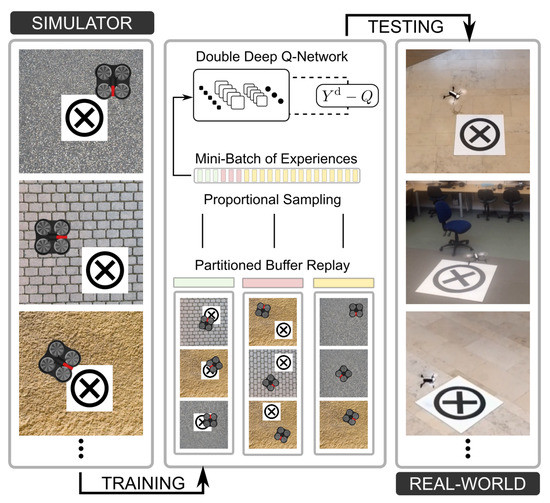
Figure 1.
System overview and deployment. Training has been performed entirely on the simulator. Three types of experiences have been collected and stored separately: correct landing (green), wrong landing (red), standard flight (yellow). Proportional sampling has been used to generate a mini-batch of experiences to train the Deep Q-Network. Testing performed in real environments.
Our contribution can be summarized as follows:
- The present work is the first to address UAV autonomous landing using a deep reinforcement learning approach with only visual inputs. The agent was trained exclusively with low-resolution grayscale images, without the need for direct supervision, hand-crafted features, or dedicated external sensors.
- A divide-and-conquer approach is used to split a complex task in sequential ones, with separate DQNs assigned to each one of them. Internal triggers are learned at training time to autonomously switch between policies. We call this new type of networks: Sequential Deep Q-Networks (SDQNs).
- A partitioned buffer replay is defined and implemented to speed up learning. This buffer stores experiences in separate partitions based on their relevance. Note that this technique can be used in other complex tasks.
- Using SDQNs, the partitioned buffer replay, and domain randomization, a commercial UAV has been trained entirely in simulation and tested in real and simulated environments. The performances are similar to human pilots and a state-of-the-art algorithm but allow harvesting the benefits of DRL such as training suitable features in different scenarios.
2. Related Work
The existing methods used for autonomous landing can be broadly grouped into three classes: sensor-fusion, infrastructure-supported, and vision-based.
The sensor-fusion methods rely on the use of multiple sensors, to gather enough data for robust pose estimation. In a recent work [15], the camera and inertial measurement unit (IMU) data were combined to reconstruct the terrain. Given the two-dimensional elevation map, it was possible to find a secure surface area for landing. In [16], the authors studied the limitations of the IMU at low frequencies and the inaccuracies of the Global Positioning System (GPS) on the horizontal plane. They showed that combining the two signals was a good compromise for robust applications. In [17], the GPS signal and the visual odometry were combined with model predictive control for landing on a moving car at a speed of 15 . Similar approaches have also been developed by teams taking part in the Mohamed Bin Zayed International Robotics Challenge (MBZIRC) 2017 competition [18,19].
Infrastructure-supported methods rely on the use of ground sensors to precisely estimate the position and the trajectory of the drone. A system based on infra-red lights has been used in [20], where a series of parallel infrared lamps are disposed in a runway. The optical filters mounted on the UAV camera captured the infrared lights and the images were forwarded to a control system for pose estimation. In [21], the authors obtained ground stereo-vision detection combining a Chan–Vese approach supplemented with an extended Kalman filter.
The vision-based approaches analyze geometric features to find the ground pad. In [22], a seven-stages vision algorithm identifies and tracks the international landing pattern in a cluttered environment, reconstructing it when partially occluded. A recent work [23] used a computer vision algorithm for detecting a moving target using only the on-board camera. The information was used to precisely estimate the UAV pose. Similarly, [24,25] adopted image-based visual servo control to track and land on a moving platform.
The aforementioned techniques have different limitations. Methods based on data integration often use information gathered from expensive sensors that usually are not available in off-the-shelf commercial platforms, or they rely on sensors that may be unavailable in specific conditions (e.g., the GPS in indoor environments). The infrastructure-supported approaches allow for obtaining an accurate estimation of the UAV pose. However, the use of external devices is not always possible because they are not always available. Vision-based methods have the advantage of relying only on internal sensors, in particular the cameras. The main limitation of these methods is that low-level features are often viewpoint-dependent and subject to failure in ambiguous cases.
The solution proposed in this work relies only on a monocular camera mounted on the UAV, without requiring any other device. Moreover, the use of DQNs as function approximators significantly improves robustness against projective transformations and marker corruption as we show in the experimental section (Section 5).
There are just a few works using DRL for the control of UAVs. In [26], the author compared different variants of DQN in learning avoidance maneuvers while navigating in a cluttered environment. A series of simulated experiments is presented in [27]. Here, the authors achieved autonomous landing using a single neural network, but, differently from our work, they significantly constrained the state space and designed a really specific reward function. In [28], the authors successfully trained a UAV to perform autonomous landing while keeping a constant descending speed. However, the method has access to a rich state representation (robot attitude, pixel distance from the marker in the camera frame, altitude) and the reward function is handcrafted and not general such as the one used in our work. A dedicated paragraph is reserved to [29] which is the most similar work to the one presented here. Instead of the DQN architecture, the authors used Deep Deterministic Policy Gradient (DDPG) [30], an actor–critic DRL algorithm that allows performing continuous control. Differently from our work, in [29], the state space has been significantly reduced and represented as a six-dimensional array combining the relative position (, , ) and acceleration (, ) of the UAV to the landing pad, together with the pressure status. These values are obtained at training time using the ground truth of the simulator, and an expensive motion capture system during the testing phase with the real platform. Our work is instead based on low-resolution grayscale images as main and only input data. This has two consequences. Our solution is more flexible and generic because it only requires a low-cost onboard camera to be effective, without the need for a complex and expensive motion capture system.
3. Problem Definition and Notation
In reinforcement learning, the goal of the agent is to maximize the discounted cumulative reward called return , where is the reward at current timestep t, while k represents future timesteps and is the discount factor. Given the current state, the agent can select an action from the action-set using an internal policy . The action brings the agent to a new state in accordance with the environmental transition model . In the particular case faced here, the transition model is not given (model free scenario). The prediction of the cumulative reward can be obtained through an action-value function adjusted during the learning phase in order to approximate , the optimal action-value function. In this work, the state is given by the image acquired by a downward-looking camera mounted on the UAV and the Convolutional Neural Network (CNN) introduced in [1] is used to approximate the Q-function. The CNN takes as input four grayscale images which are processed by three convolutional layers and two fully connected layers. Rectified linear units are used as activation functions. The first convolution has 32 kernels of with a stride of 2, the second layer has 64 kernels of with strides of 2, and the third layer convolves 64 kernels of with a stride of 1. The fourth layer is a fully connected layer of 512 units followed by the output layer that has a unit for each valid action (backward, right, forward, left, stop, descent, land). Each action is represented by a three-dimensional vector , expressed in the robot frame that allows moving the drone with a specific velocity on the three axes. A graphical representation of the network is presented in Figure 2.
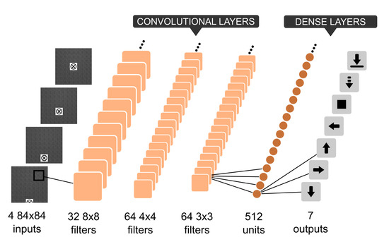
Figure 2.
The convolutional network used to approximate the Q-function. It receives in input four gray scale images, and outputs seven actions.
In this work, the landing problem is divided into landmark alignment and vertical descent. The reason behind this choice is better justified in the next section (Section 4); here, we introduce the notation and the loss functions used at training time. The landmark alignment requires an exploration of the horizontal -plane at a fixed altitude of 20 , where the UAV has to horizontally shift in order to align its body frame with the marker. In the vertical descent phase, the vehicle has to reduce the distance from the marker using vertical movements. Moreover, the drone has to shift on the -plane in order to keep the marker centered. We now describe both phases in more detail.
3.1. Landmark Alignment
In this phase, the reasonable assumption of a flight at fixed-altitude was made. The horizontal alignment with the landmark is obtained through shifts in the -plane. To adjust , the parameters of the DQN, the following loss function was minimized
with being a data-set of experiences which are uniformly sampled. The network is used to estimate actions at run-time, whereas is defined as
with the network used to generate the target and constantly updated. The parameters of the target network are updated every C steps and synchronized with . Following standard practice, the experiences in the data-set are collected in a preliminary phase using a random policy.
3.2. Vertical Descent
This phase is a form of Blind Cliff-walk [31], where the agent has to take the right action to progress through a sequence of N states and finally get a positive or a negative reward. The intrinsic structure of the problem makes it extremely difficult to obtain a positive reward because the target-zone is only a small portion of the state space. As a consequence, the buffer replay does not contain enough positive experiences, leading to unstable control policy. To solve this issue, we introduced a new form of buffer replay called partitioned buffer replay. This new type of buffer discriminates between rewards and guarantees a fair sampling between positive, negative and neutral experiences. Additional details about the partitioned buffer replay are provided in Section 4.2.
Another issue connected with the reward sparsity is the utility overestimation. During our preliminary studies, this problem was observed to be affecting the vertical descent phase. The Q-max value (the highest utility returned by the Q-network) rapidly increased, overshooting the maximum possible utility of . The overestimation was associated with all the actions but the trigger. This is because the trigger leads to a terminal state; therefore, its utility is updated without using the operator, which was found to be the responsibility of the overestimation in deep Q-learning. In our case, the overestimated utilities of the four horizontal movements (grown up to after frames) were higher than the non-overestimated utility associated with the trigger (stably converged to ). As a result, the drone moved on top of the marker but it did not engage the trigger. A solution to the overestimation has been recently proposed and has been called double DQN [13]. The target estimated through double DQN is defined as follows:
Note that the operator in Equation (2) uses the same values both to select and to evaluate an action; therefore, it is more likely to select overestimated values, whereas, in Equation (3), the divergence is mitigated using over Q at the next time step, resulting in faster convergence and increased stability.
3.3. Vehicle Characteristics
The platform used in this work is the Parrot Bebop 2 (produced by Parrot Drones SAS, Paris, France), a commercial off the shelf quadcopter. Regarding its dynamics, the UAV can be seen as a rigid body with 6 degrees of freedom (DOF) able to generate the necessary forces and moments for moving [32]. The equations of motion are expressed in the body-fixed reference frame [33]
where and represent the linear and angular velocities of the UAV in . F is the translational force combining gravity, thrust and other components, while is the inertial matrix subject to F and torque vector . The orientation of the UAV in the air is given by a rotation matrix R from to the inertial reference frame :
where is the vector of Euler angles and s and c are abbreviations for and . Given the transformation from the body frame to the inertial frame , the gravitational force and the translational dynamics in are
where g is the gravitational acceleration, is the resulting force in , and are the position and velocity in . The body frame follows a right-handed z-up convention such that the positive x-axis is oriented along the forward direction of travel.
4. Proposed Method
4.1. Sequential Deep Q-Networks (SDQN)
The main issues in applying DRL to robotics are related to the large size of the state and action spaces and to reward sparsity which often makes it difficult to learn a policy. In robotics, the agent needs to explore relevant portions of the environment and to perform different actions in order to receive useful feedback. In most cases, the environment is large and the reward infrequent; therefore, learning becomes difficult. In order to overcome these issues, we propose a simple method which consists of splitting the main task into sub-tasks, such that both state and action spaces are reduced. A similar approach has been described in hierarchical reinforcement learning [34] where a set of sub-policies, called options, are available to the agent in specific states. The options control the agent in sub-regions of a core Markov Decision Process (MDP) called semi-MDPs. In an MDP, at each time step t, the agent receives the state , performs an action sampled from the action space , and receives a reward given by a reward function . In the present work, the core MDP is divided into multiple isolated instances, with each instance being a proper MDP. The auxiliary MDPs are therefore connected in an ordered sequence thanks to shared states and specific actions, called triggers, which allow switching from one MDP to the following one. When calling the trigger in a shared state, the agent receives a reward which is equal to the maximal reward of the core MDP. The design of the individual auxiliary MDPs requires some knowledge about the overall task and, for this reason, is left to the designer. The advantage of reinterpreting semi-MDPs as MDPs is that it allows using standard Q-learning to train the agent. If we divide the state space and the action space in J partitions, we can associate a specialized Q-function to each sub-task
Since the Q-functions are executed sequentially, one after the other, we call the overall function a Sequential Q-function, and, when this is parameterized by a deep neural network, we call it a Sequential Deep Q-Network (SDQN). The transition from one Q-function to the other is managed by a particular action called trigger and a state called the transition state. More formally, we define a trigger as an additional action allocated to each one of the partitions
When the trigger is engaged in its transition state , the agent gets maximal reward and the next function in the sequence is called; otherwise, it gets a minimal reward and the episode terminates:
In the particular case of autonomous drone landing, we propose to divide the task into landmark alignment and vertical descent, as shown in the flowchart of Figure 3. The alignment requires an exploration of the horizontal -plane at a fixed altitude of 20 , where the UAV has to shift in order to align its body frame with the marker. In the vertical descent phase, the vehicle has to reduce the distance from the marker using vertical movements. Moreover, the drone can laterally shift to keep the marker centered. Splitting the overall task into two gives more flexibility while keeping the problem of exploring a large state space still tractable. As proof of this, we trained a single DQN to perform both alignment and descending. Given the size of the combined state spaces, the network did not converge to a stable policy. The accumulated reward is reported in Section 5 and marked as standard DQN [1].
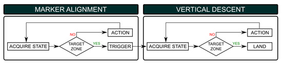
Figure 3.
Flowchart representing the marker alignment and vertical descent phases.
Here, it is fundamental to clarify a crucial point. In a simulated environment, it may be possible to use the distance between the UAV and the marker to produce constant feedback. However, this is a form of privileged information that can be expensive to obtain in the real word without specialized hardware for precise distance estimation, like the one used in [29]. This is the main reason why this information has not been used in our experiments. We wanted the method to be flexible, such that it would be possible to train in the simulator and fine-tune in the real world giving just minimal feedback to the system (e.g., sparse rewards). An algorithm that works in the worst conditions will likely work in more favorable conditions, whereas the opposite is not guaranteed.
4.2. Partitioned Buffer Replay
Tasks with a sparse and time-delayed reward make it difficult for the agent to get constant positive feedback. As a consequence, the buffer replay can be unbalanced, leading neutral transition (those associated with a non-relevant reward) to be sampled with a higher probability than positive and negative ones.
In our case, the vertical descent is affected by the problem of reward sparsity which causes an underestimation of the utilities associated with the triggers. In [35], it has been shown that dividing the experiences into two groups based on a priority value can alleviate the problem. The method we propose in this work is an extension of K groups. A different approach has been taken in [31], where experiences are sampled using a weight proportional to the temporal difference error, with important transitions sampled more frequently. The main drawback of this approach is the introduction of another layer of complexity which is not justified where a clear distinction between positive and negative rewards occurs. Moreover, this method requires to update the priorities, whereas in our case the update is done in constant time. This issue does not significantly affect performances on the standard benchmarks, but it has a relevant effect on robotics applications, where there is a high cost in obtaining experiences.
Following the same notation introduced before, the buffer replay is defined as and an experience as . At each iteration i, we uniformly sample from it a batch where s is the current state, a the action performed, r the reward received and the new state. The scope of this buffer replay is mainly to randomize samples, breaking the correlation, and reducing the variance [36]. In order to create a partitioned buffer replay, the reward space is divided into K partitions
associating with each partition a different dataset
Experiences are iteratively sampled from each one of the K partition with a certain fraction and stored in the training batch. In our particular case, there are three partitions, each one associated with a different reward: containing positive experiences (), containing negative experiences (), and for neutral experiences (). The fraction of experiences associated with each one of the partitions is defined as , , and . When using a partitioned buffer replay, there is a substantial increase in the available number of positive and negative experiences. In order to clarify the advantages of using a partitioned buffer replay, we provide here a concrete example, comparing it to a standard buffer replay [1]. We implemented a standard buffer replay of size and we accumulated transitions with a random agent in a basic environment (see Section 5). The total number of positive experiences accumulated in the buffer is only 343 and the number of negative experiences 2191. The remaining 17,466 experiences, corresponding to of the total, are neutral (low relevance). As a consequence, at training time, the mini-batch of experiences sampled from the standard buffer would not contain enough significant experiences to effectively train the policy. On the other hand, our partitioned buffer replay stores experiences in a distinguishable way in different partitions based on the associated reward. If we accumulate the same amount of experiences () with a random agent using a partitioned buffer replay (size for neutral partition, and size for positive and negative partitions), the total number of positive experiences collected is 1352 and the number of negative experiences 9270, which are significantly higher than the standard counterpart. At training time, we can sample experiences from all the partitions of the buffer and guarantee that positive and negative experiences (the most significant) are always present within the mini-batch.
4.3. Training through Domain Randomization
The biggest challenge in robot learning is the gap between the design in a simulated environment and the deployment in the real world. Domain transfer techniques have been recently identified as a solution for reducing this gap, with one of the most effective approaches being Domain Randomization (DR) [10]. This method consists of randomizing the visual and physical properties of the simulator during the training phase. Here, DR is adopted to train the control policy of the UAV in simple simulated environments and then test it in complex unseen environments (both simulated and real). The remarkable property of this approach is that if the variability is significant enough, models trained in simulation generalize to the real world with no additional training. This can be achieved by changing environmental properties (e.g., visual textures and physics parameters) at training time.
4.4. Suitability of the Method to Robotics Applications
Here, we would like to briefly discuss possible applications of the method we have described. SDQNs are able to effectively and flexibly tackle sequential problems; for this reason, they can be used in all those robotics applications where there is a large state space with a clear distinction in separable sub-spaces. Note that this assumption is rather common in robotics; for instance, problems that fall into this category are: goal-oriented navigation (not only aerial), automation of assembly lines, manipulation with pick-and-place. In all these cases, it is possible to easily find sub-tasks that can be isolated and assigned to a separate policy. Another advantage of SDQNs stands in their modular design, and each sub-policy is in fact an independent block which can be used in other applications as part of a different policy. Moreover, each one of these blocks can be rapidly (re)trained in simulation or fine-tuned on a new problem, without the need to intervene on the overall policy. This considerably shortens the deployment time while simplifying system debugging and updating, with obvious advantages for commercial applications. The possibility of using domain randomization is another advantage of our method when it comes to real-world robotics scenarios. Often, it is not possible to use data from the final application to improve the performance of the robot before the deployment in a specific use case. For instance, the navigation in a disaster site is more challenging than navigation in a standard environment where the robot can be easily trained. However, data from disaster sites are difficult to obtain beforehand. Using domain randomization, it is possible to fine-tune the policy on a large variety of simulated disaster sites and then deploy a robust policy in the real world.
5. Experiments
In this section, the methodology and the results obtained by SDQN in the two phases are presented. In both training and testing, the same environment (Gazebo , ROS Kinetic) and drone (Parrot BeBop 2, produced by Parrot Drones SAS, Paris, France) were used. The marker used in the experiments is the same adopted in the MBZIRC competition, consisting of a black cross within a black circle on a white background, which can be considered the current standard. To understand the impact of environmental variability on the results, we designed two experimental conditions with two different SDQNs. The first was trained using only a single uniform asphalt texture (SDQN), while the second was trained with seven different groups of textures using domain randomization (SDQN-DR). The textures are: asphalt, brick, grass, pavement, sand, snow, and soil (Figure 4h). Both SDQN and SDQN-DR use the same neural networks as sequential components (Figure 2).
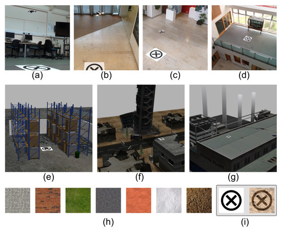
Figure 4.
Real environments: (a) laboratory, (b) small hall, (c) large hall, (d) mezzanine. Photo-realistic environments: (e) warehouse, (f) disaster site, (g) power-plant. (h) Textures: pavement, brick, grass, asphalt, sand, snow, soil. (i) Marker and corrupted marker.
5.1. Methods
During the marker alignment phase, the UAV flies at a fixed altitude of 20 which is kept for the duration of the episode. This expedient reduces the state space to explore and keeps the marker within the camera field of view. Taking inspiration from the no-operation introduced in [1], each action is repeated for 2 and then interrupted, leading to an approximate shift of 1 . This choice has been taken to increase the variance between two consecutive observations, stabilizing the learning. The frames from the camera are acquired between two actions (at a frequency of ) when the vehicle is stationary. The training environment is represented by a uniform texture of size with the landmark positioned in the center. The environment contains a flying and a target zone (Figure 5). At the beginning of each episode, the drone is spawned at 20 of altitude inside the perimeter of the larger bounding box () with a random position and orientation. A positive reward of is given when the drone activates the trigger in the target zone, and a negative reward of is given if the drone activates the trigger outside the target-zone. A negative cost of living of is applied in all the other cases. A time limit of 40 (20 steps) is used to stop the episode and start a new one. In the SDQN-DR condition, domain randomization is used to change the ground texture every 50 episodes and to randomly sample between the 71 textures available in the training set. The target and policy networks are synchronized every 10,000 frames following the original approach [1]. The agent has five possible actions available: forward, backward, left, right, trigger. The additional action move-down was used during vertical descent. The action selected is repeated for 2 ; then, the drone is left stationary and a new action is sampled. The buffer replay was filled before the training phase with frames using a random policy. The SDQN and SDQN-DR were trained for frames. An -greedy policy was used, with decayed linearly from 1 to over the first frames and fixed at thereafter.
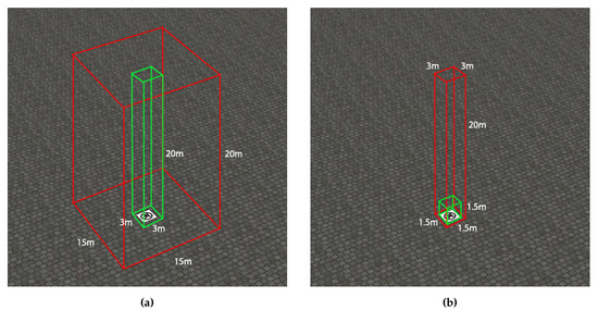
Figure 5.
Flying-zone (red) and target-zone (green) for landmark alignment (a) and vertical descent (b).
In the vertical descent phase, to encourage the UAV to descend above the marker, during the -greedy selection, the action was sampled from a non-uniform distribution with move-down having a probability and the other N actions having a probability . Exploring-start was adopted to generate the UAV at different altitudes and to ensure a wider exploration of the state space. We used the partitioned buffer replay described in Section 4.2. Compared with the marker alignment phase, the state-space for the vertical descent is much larger and more expensive to explore. For this reason, we decided to sub-sample uniformly only 20 textures among the 71 available within the training set. In the vertical descent, the target and the policy networks are synchronized every frames following the recommendations in [13]. For the partitioned buffer replay, it was chosen , , and . At the beginning of each episode, the drone is spawned with a random orientation inside a bounding box of size , which corresponds to the target area of the landmark alignment phase. Given this large dimension, a time limit of 80 (40 steps) is used to stop the episode and start a new one. A positive reward of was given only when the drone entered in a target-zone of size , centred on the marker (Figure 5). If the drone descended above outside the target-zone, a negative reward of was given. A cost of living of was applied at each time step. Before the training, the buffer replay was filled using a random policy with neutral experiences, negative experiences and positive experiences.
For both phases, the discount factor was set to . As an optimizer, we used the RMSProp algorithm with a batch size of 32. The SDQN was implemented in Tensorflow. The simulations were performed on a workstation Intel i7 with 8 cores (produced by Intel Corporation, Santa Clara, CA, USA). processor, 32 GB of RAM, and the NVIDIA Quadro K2200 (produced by Nvidia Corporation, Santa Clara, CA, USA) as the graphical processing unit. On this hardware, the training took days to complete for the marker alignment phase and for the vertical descent one, with the physic engine running real-time. In addition to the hardware already mentioned, a separate machine was used to collect preliminary experiences. This machine is a multi-core workstation with 32 GB of RAM and a GPU NVIDIA Tesla K-40 (produced by Nvidia Corporation, Santa Clara, CA, USA).
A comparison with human subjects has also been performed. The data were collected with the help of 10 volunteers (6 males and 4 females, average age 27) who used the same control actions available to the other agents. After an initial training phase to familiarize themselves with the task, the real test started. The objective was to move the UAV above the marker and then engage the trigger when inside the target-zone. All the candidates were supplied with only low-resolution gray-scale images as those used in input for the networks. The frame rate between two consecutive images was kept fixed at . The same expiration rate adopted in the training phase was applied to each episode to better compare the results with the other methods. Five trials were performed for each one of the environments in the test set (randomly sampled). A landing attempt was declared as failed when the time limit expired or when the subject engaged the trigger outside the target-zone.
5.2. Results
First, we analyze the training statistics of SDQN, SDQN-DR, and standard DQN. Those are summarized in Figure 6-bottom for marker alignment, and Figure 7-bottom for the vertical descent. In both figures, the cumulated reward for SDQN (blue curve) and SDQN-DR (red curve) increased stably without any anomaly, meaning that the agents learned how to successfully accomplish the task on the training environments. The reward curve for the standard DQN [1] condition (green) did not increase significantly and the resulting policy was unable to engage the trigger inside the target-zone.
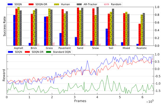
Figure 6.
Results for the marker alignment phase. Top: success rate in different textures and conditions. Bottom: accumulated average reward per episode for Sequential Deep Q-Network (SDQN, blue line), Sequential Deep Q-Network with domain randomization (SDQN-DR, red line), and standard Deep Q-Network [1] (DQN, green).
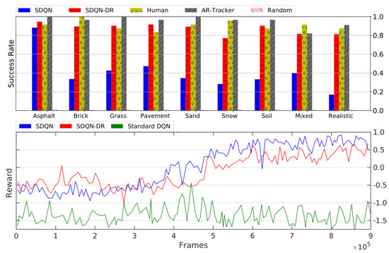
Figure 7.
Results for the vertical descent phase. Top: success rate in different textures and conditions. Bottom: accumulated average reward per episode for Sequenital Deep Q-Network (SDQN, blue line), Sequential Deep Q-Network with domain randomization (SDQN-DR, red line), and standard Deep Q-Networks [1] (DQN, green line).
In the test phase, we compared the performance of various methods: SDQN, SDQN-DR, a random agent, a state-of-the-art AR-tracker algorithm [37], and human pilots. We performed a series of four tests for both marker alignment and vertical descent. Those tests and the results obtained are summarized here:
- Uniform. The first test was performed on 21 unknown uniform textures belonging to the same categories as the training set. For the marker alignment phase, SDQN-DR has an accuracy of , while SDQN obtains a lower score (). The human performance is , the AR-tracker has a score of , and the random agent of . In the vertical descent phase, SDQN-DR achieved an accuracy of , for SDQN, for humans, and for the AR-tracker. Table 1 reports a comparison between our method (SDQN-DR) and human pilots. For the human subjects, the average time required to accomplish the task was 24 (marker alignment) and 46 (vertical descent), whereas for the SDQN-DR was only 12 and 38 . The humans were significantly slower but more accurate than the artificial agents. This result highlights a difference in strategy between humans and artificial agents, therefore the performance of the two groups must be compared carefully.
 Table 1. Comparison of our method (SDQN-DR) and humans for: success rate (SR, percentage), average time (T, seconds), average distance when trigger is engaged (X and Y, meters). Best results are in bold.Note that in our method the trade-off between accuracy and speed can be tuned by the cost-of-living (neutral reward), with higher values pushing the agent to complete the task faster (but with a lower accuracy).
 - Corrupted. The second test was performed on the same 21 unknown textures but using a marker which has been corrupted through a semi-transparent dust-like layer (Figure 4i). In this condition, we observed a significant drop in the AR-tracker performances from to (marker alignment) and from to (vertical descent). This result can be explained by the fact that the underlying template matching algorithm failed in identifying the corrupted marker. Under the same condition, the SDQN-DR performed well, with a limited drop in performance from to (marker alignment) and from to (vertical descent), showing to be more robust to marker corruption.
- Mixed. The third test was done randomly sampling 25 textures from the test set and mixing them in a mosaic-like composition. In the marker alignment phase, SDQN-DR had a success rate of , SDQN , human pilots and the AR-tracker . In addition, for the vertical descent, we registered worst performances for all the agents (SDQN-DR = , SDQN = , Humans = , Random = , AR-tracker = ).
- Photo-Realistic. The fourth and last test has been done on three photo-realistic environments: warehouse, disaster site, and a power-plant (Figure 4e,g). In addition, here we observed a generic drop in performance for marker alignment (SDQN-DR = , SDQN = , Human = , Random = , AR-tracker = ) and vertical descent (SDQN-DR = , SDQN = , Human = , Random = , AR-tracker = ), showing how completing the task in a complex environment is more difficult for all agents.
The previous results are reported in Table 2 to facilitate the comparison between methods. Additionally, we report a comparison on every texture in Figure 6-top for marker alignment, and Figure 7-top for vertical descent. Note that, our method (SDQN-DR) reports the best score overall (78% marker alignment, 75% vertical descent), substantially outperforming a state-of-the-art AR-Tracker [37] (65% marker alignment, 68% vertical descent) as showed in Table 2.
Table 2.
Success rate (percentage) at test time on marker alignment and vertical descent for: random agent, AR-Tracker, Sequential Deep Q-Network without domain randomization (SDQN), Sequential Deep Q-Network with domain randomization (SDQN-DR). Test performed on: uniform texture, marker corrupted, mixed textures, photo-realistic environments. Average total performance indicated as TOT. Best results are highlighted in bold.
6. Real World Implementation
Training and testing only in the simulator is not enough to assess the quality of a method. Simulated data usually have poor fidelity and the components that make a real experiments difficult, such as the physics and the environmental conditions (light, winds etc) usually not being modeled in a proper way. For these reasons, we performed a series of tests in real environments. However, before testing the proposed approach in the real world, a few additional tests have been performed to collect accurate statistics regarding the robustness against variations in altitudes and drift injection. In the first test, SDQN-DR was tested for marker alignment on the same environments but at different altitudes (respectively, 20 , 15 , and 10 ). The accuracy increased at 15 (95%) and 10 (93%), with respect to the accuracy at the training altitude of 20 (91%). This can be explained by the fact that at lower altitudes the marker is more visible and the state space smaller. In the second test, we measured the performance of our method against noise injection in the action-space, we modified the action repetition time (and as consequence the vehicle shift) from the value used during training (2 ) to three additional values: 1 , , . The results confirmed that the network was able to generalize effectively achieving results above in most of the conditions (Table 3). SDQN-DR was also tested against different drift values, modeled as noise in the velocity space. The drift consisted of a scalar sampled from a uniform distribution in the range () and accumulated for a time of 5 . Four conditions with a different value of a have been tested , , , . In addition, in this case, the results showed that the SDQN-DR was able to effectively generalize, even though the training was performed without drift.
Table 3.
Success rate (percentage) of Sequential Deep Q-Network with domain randomization (SDQN-DR) against noise injection in action space and drift.
Finally, we measured the performance of the agent in the real world. In this test, additional factors other than motion drift played an important role—for instance, the high number of unknown objects and features present in the camera image, the noise caused by natural light and motion blur. All of these factors added a considerable domain shift compared to the training phase. The effect of lighting conditions has not been directly quantified, but it has been qualitatively identified. In particular, we noticed two sources of interference, the first given by smooth surfaces (e.g., glass, pavement, tables, etc), and the second given by the presence of shadows (not present at training time due to the use of a uniform light). Both of those effects introduced artifacts into the raw image acquired by the camera, sometimes affecting the correct identification of the landmark. The vertical descent tests were performed in four environments: laboratory, small hall, large hall and mezzanine (Figure 4a–d). A total of 40 flights were equally distributed in the four environments. The flight attempts regarding the marker alignment were possible only in one of those environments (mezzanine, Figure 4d) which was the only space that allowed the UAV to safely reach an altitude of at least 15 . In this case, a total of 10 flights was performed.
The experiments on the marker alignment phase were successful of the times, whereas, in the vertical descent, the system obtained an overall success rate of . Remarkably, even when the drone was not able to land, the flight was interrupted due to the expiration time (a maximum of 40 steps allowed) and not even once the drone landed outside the pad. This kind of policy spontaneously emerged because landing outside the pad was penalized by a negative reward at training time in the simulator. A snapshot of the experiments is reported in Figure 8.
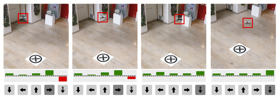
Figure 8.
Snapshots of the descending phase with the utility distribution over all the actions. Descent has a negative utility (red bar) when the drone is not centred on the marker.
7. Discussion and Conclusions
In this work, DRL was used for the first time to implement a system for autonomous landing a UAV on a fixed pad relying solely on raw visual inputs. The entire system is based on a Sequential Deep Q-Network, composed of two DQNs that control the UAV in two phases: landmark alignment and vertical descent. Using domain randomization, the DQNs were trained only in simulation using simple uniform textures and later tested in complex environments, both simulated and real. The overall performances are comparable with a state-of-the-art AR-tracker algorithm and human pilots. More precisely, the system is faster than humans in reaching the pad and more robust to marker corruption than the AR-tracker. The most remarkable outcome is that the networks were able to generalize to real environments despite the training was performed only in simulation and with a limited subset of textures. One of the limitations of this approach is the possible mismatch between performances at training and test time when there is a considerable domain shift in the two phases due to different environmental conditions (e.g., different lighting and drift). In future work, we aim at improving the results taking into account these factors during the simulated training phase so to improve the performances in the real world. In conclusion, the promising results reported in this paper show that raw visual inputs can be successfully combined with deep reinforcement learning for solving challenging robotics tasks such as the landing of a UAV.
Author Contributions
R.P. and M.P. conceived and designed the Sequential Deep Q-Network method, realized the experiments, analyzed the data, and wrote the article. R.P. designed and implemented the controller of the drone (both real and simulated). M.P. defined and implemented the partitioned buffer replay and the reinforcement learning stack. M.H. and G.N. provided supervision, guidance, and the funding to sustain the project. All authors have read and agreed to the published version of the manuscript.
Funding
The research leading to these results has received funding from EPSRC under grant agreement EP/R02572X/1 (National Center for Nuclear Robotics).
Conflicts of Interest
The authors declare no conflict of interest.
References
- Mnih, V.; Kavukcuoglu, K.; Silver, D.; Rusu, A.A.; Veness, J.; Bellemare, M.G.; Graves, A.; Riedmiller, M.; Fidjeland, A.K.; Ostrovski, G.; et al. Human-level control through deep reinforcement learning. Nature 2015, 518, 529–533. [Google Scholar] [CrossRef] [PubMed]
- Gu, S.; Holly, E.; Lillicrap, T.; Levine, S. Deep reinforcement learning for robotic manipulation with asynchronous off-policy updates. In Proceedings of the 2017 IEEE International Conference on Robotics and Automation (ICRA), Singapore, Singapore, 29 May–3 June 2017; pp. 3389–3396. [Google Scholar]
- Andrychowicz, O.M.; Baker, B.; Chociej, M.; Jozefowicz, R.; McGrew, B.; Pachocki, J.; Petron, A.; Plappert, M.; Powell, G.; Ray, A.; et al. Learning dexterous in-hand manipulation. Int. J. Rob. Res. 2020, 39, 3–20. [Google Scholar] [CrossRef]
- Tai, L.; Paolo, G.; Liu, M. Virtual-to-real deep reinforcement learning: Continuous control of mobile robots for mapless navigation. In Proceedings of the 2017 IEEE/RSJ International Conference on Intelligent Robots and Systems (IROS), Vancouver, BC, Canada, 24–28 September 2017; pp. 31–36. [Google Scholar]
- Zhu, Y.; Mottaghi, R.; Kolve, E.; Lim, J.J.; Gupta, A.; Fei-Fei, L.; Farhadi, A. Target-driven visual navigation in indoor scenes using deep reinforcement learning. In Proceedings of the 2017 IEEE International Conference on Robotics and Automation (ICRA), Singapore, Singapore, 29 May–3 June 2017; pp. 3357–3364. [Google Scholar]
- Kahn, G.; Villaflor, A.; Ding, B.; Abbeel, P.; Levine, S. Self-supervised deep reinforcement learning with generalized computation graphs for robot navigation. In Proceedings of the 2018 IEEE International Conference on Robotics and Automation (ICRA), Brisbane, QLD, Australia, 21–25 May 2018; pp. 1–8. [Google Scholar]
- Ha, D.; Schmidhuber, J. Recurrent world models facilitate policy evolution. In Proceedings of the Advances in Neural Information Processing Systems, Montréal, QC, Canada, 2–8 December 2018; pp. 2450–2462. [Google Scholar]
- Thabet, M.; Patacchiola, M.; Cangelosi, A. Sample-efficient Deep Reinforcement Learning with Imaginary Rollouts for Human-Robot Interaction. arXiv 2019, arXiv:1908.05546. [Google Scholar]
- Zhang, F.; Leitner, J.; Milford, M.; Corke, P. Modular deep q networks for sim-to-real transfer of visuo-motor policies. arXiv 2016, arXiv:1610.06781. [Google Scholar]
- Tobin, J.; Fong, R.; Ray, A.; Schneider, J.; Zaremba, W.; Abbeel, P. Domain randomization for transferring deep neural networks from simulation to the real world. In Proceedings of the 2017 IEEE/RSJ International Conference on Intelligent Robots and Systems (IROS), Vancouver, BC, Canada, 24–28 September 2017; pp. 23–30. [Google Scholar]
- Tobin, J.; Biewald, L.; Duan, R.; Andrychowicz, M.; Handa, A.; Kumar, V.; McGrew, B.; Ray, A.; Schneider, J.; Welinder, P.; et al. Domain randomization and generative models for robotic grasping. In Proceedings of the 2018 IEEE/RSJ International Conference on Intelligent Robots and Systems (IROS), Madrid, Spain, 1–5 October 2018; pp. 3482–3489. [Google Scholar]
- Polvara, R.; Patacchiola, M.; Sharma, S.; Wan, J.; Manning, A.; Sutton, R.; Cangelosi, A. Toward End-to-End Control for UAV Autonomous Landing via Deep Reinforcement Learning. In Proceedings of the 2018 International Conference on Unmanned Aircraft Systems (ICUAS), Dallas, TX, USA, 12–15 June 2018; pp. 115–123. [Google Scholar] [CrossRef]
- Van Hasselt, H.; Guez, A.; Silver, D. Deep Reinforcement Learning with Double Q-Learning. In Proceedings of the Thirtieth AAAI Conference on Artificial Intelligence, Phoenix, AZ, USA, 12–17 February 2016; pp. 2094–2100. [Google Scholar]
- Thrun, S.; Schwartz, A. Issues in using function approximation for reinforcement learning. In Proceedings of the 1993 Connectionist Models Summer School, 1st ed.; Psychology Press: London, UK, 1993. [Google Scholar]
- Forster, C.; Faessler, M.; Fontana, F.; Werlberger, M.; Scaramuzza, D. Continuous on-board monocular-vision-based elevation mapping applied to autonomous landing of micro aerial vehicles. In Proceedings of the 2015 IEEE International Conference on Robotics and Automation (ICRA), Seattle, WA, USA, 26–30 May 2015; pp. 111–118. [Google Scholar]
- Sukkarieh, S.; Nebot, E.M.; Durrant-Whyte, H.F. A high integrity IMU/GPS navigation loop for autonomous land vehicle applications. IEEE Trans. Robo. Autom. 1999, 15, 572–578. [Google Scholar] [CrossRef]
- Baca, T.; Stepan, P.; Saska, M. Autonomous landing on a moving car with unmanned aerial vehicle. In Proceedings of the 2017 European Conference on Mobile Robots (ECMR), Paris, France, 6–8 September 2017; pp. 1–6. [Google Scholar]
- Beul, M.; Houben, S.; Nieuwenhuisen, M.; Behnke, S. Fast autonomous landing on a moving target at MBZIRC. In Proceedings of the 2017 European Conference on Mobile Robots (ECMR), Paris, France, 6–8 September 2017; pp. 1–6. [Google Scholar]
- Bähnemann, R.; Pantic, M.; Popović, M.; Schindler, D.; Tranzatto, M.; Kamel, M.; Grimm, M.; Widauer, J.; Siegwart, R.; Nieto, J. The ETH-MAV Team in the MBZ International Robotics Challenge. J. Field Rob. 2009, 36, 78–103. [Google Scholar] [CrossRef]
- Gui, Y.; Guo, P.; Zhang, H.; Lei, Z.; Zhou, X.; Du, J.; Yu, Q. Airborne vision-based navigation method for uav accuracy landing using infrared lamps. J. Intell. Rob. Syst. 2013, 72, 197. [Google Scholar] [CrossRef]
- Tang, D.; Hu, T.; Shen, L.; Zhang, D.; Kong, W.; Low, K.H. Ground stereo vision-based navigation for autonomous take-off and landing of uavs: A chan-vese model approach. Int. J. Adv. Rob. Syst. 2016, 13, 67. [Google Scholar] [CrossRef]
- Lin, S.; Garratt, M.A.; Lambert, A.J. Monocular vision-based real-time target recognition and tracking for autonomously landing an UAV in a cluttered shipboard environment. Autono. Robots 2017, 41, 881–901. [Google Scholar] [CrossRef]
- Falanga, D.; Zanchettin, A.; Simovic, A.; Delmerico, J.; Davide, S. Vision-based Autonomous Quadrotor Landing on a Moving Platform. In Proceedings of the 2017 IEEE International Symposium on Safety, Security, and Rescue Robotics (SSRR), Shanghai, China, 11–13 October 2017; pp. 200–207. [Google Scholar]
- Serra, P.; Cunha, R.; Hamel, T.; Cabecinhas, D.; Silvestre, C. Landing of a Quadrotor on a Moving Target Using Dynamic Image-Based Visual Servo Control. IEEE Trans. Rob. 2016, 32, 1524–1535. [Google Scholar] [CrossRef]
- Lee, D.; Ryan, T.; Kim, H.J. Autonomous landing of a VTOL UAV on a moving platform using image-based visual servoing. In Proceedings of the 2012 IEEE International Conference on Robotics and Automation, Saint Paul, MN, USA, 14–18 May 2012; pp. 971–976. [Google Scholar]
- Kersandt, K. Deep Teinforcement Learning as Control Method for Autonomous Uavs. Master’s Thesis, Universitat Politècnica de Catalunya, Catalonia, Spain, February 2017. [Google Scholar]
- Xu, Y.; Liu, Z.; Wang, X. Monocular Vision based Autonomous Landing of Quadrotor through Deep Reinforcement Learning. In Proceedings of the 2018 37th Chinese Control Conference (CCC), Wuhan, China, 25–27 July 2018; pp. 10014–10019. [Google Scholar] [CrossRef]
- Lee, S.; Shim, T.; Kim, S.; Park, J.; Hong, K.; Bang, H. Vision-Based Autonomous Landing of a Multi-Copter Unmanned Aerial Vehicle using Reinforcement Learning. In Proceedings of the 2018 International Conference on Unmanned Aircraft Systems (ICUAS), Dallas, TX, USA, 12–15 June 2018; pp. 108–114. [Google Scholar] [CrossRef]
- Rodriguez-Ramos, A.; Sampedro, C.; Bavle, H.; De La Puente, P.; Campoy, P. A deep reinforcement learning strategy for UAV autonomous landing on a moving platform. J. Intell. Rob. Syst. 2019, 93, 351–366. [Google Scholar] [CrossRef]
- Lillicrap, T.P.; Hunt, J.J.; Pritzel, A.; Heess, N.; Erez, T.; Tassa, Y.; Silver, D.; Wierstra, D. Continuous control with deep reinforcement learning. arXiv 2015, arXiv:1509.02971. [Google Scholar]
- Schaul, T.; Quan, J.; Antonoglou, I.; Silver, D. Prioritized experience replay. arXiv 2015, arXiv:1511.05952. [Google Scholar]
- Nonami, K.; Kendoul, F.; Suzuki, S.; Wang, W.; Nakazawa, D. Autonomous Flying Robots: Unmanned Aerial Vehicles and Micro Aerial Vehicles, 1st ed.; Springer: Berlin, Germany, 2010. [Google Scholar]
- Goldstein, H. Classical Mechanics, 2nd ed.; World Student Series; Addison-Wesley: Reading, MA, USA; Menlo Park, CA, USA; Amsterdam, The Netherland, 1980. [Google Scholar]
- Barto, A.G.; Mahadevan, S. Recent advances in hierarchical reinforcement learning. Discrete Event Dyn. Syst. 2003, 13, 341–379. [Google Scholar] [CrossRef]
- Narasimhan, K.; Kulkarni, T.; Barzilay, R. Language understanding for text-based games using deep reinforcement learning. arXiv 2015, arXiv:1506.08941. [Google Scholar]
- WawrzyńSki, P.; Tanwani, A.K. Autonomous reinforcement learning with experience replay. Neural Netw. 2013, 41, 156–167. [Google Scholar] [CrossRef] [PubMed]
- Polvara, R.; Sharma, S.; Wan, J.; Manning, A.; Sutton, R. Towards autonomous landing on a moving vessel through fiducial markers. In Proceedings of the 2017 European Conference on Mobile Robots (ECMR), Paris, France, 6–8 September 2017; pp. 1–6. [Google Scholar] [CrossRef]
© 2020 by the authors. Licensee MDPI, Basel, Switzerland. This article is an open access article distributed under the terms and conditions of the Creative Commons Attribution (CC BY) license (http://creativecommons.org/licenses/by/4.0/).