Article

On Using Inertial Measurement Units for Solving the Direct Kinematics Problem of Parallel Mechanisms

Workgroup on System Technologies and Engineering Design Methodology, Hamburg University of Technology, 21073 Hamburg, Germany
Robotics 2019, 8(4), 99; https://doi.org/10.3390/robotics8040099
Submission received: 22 October 2019 / Revised: 14 November 2019 / Accepted: 27 November 2019 / Published: 29 November 2019

Abstract

:
In this paper, we investigate the accuracy and the computational efficiency of an IMU-based approach for solving the direct kinematics problem of parallel mechanisms with length-variable linear actuators under dynamic conditions. By avoiding to measure the linear actuators’ lengths and by using orientations instead, a comprehensive, low-cost sensor structure can be obtained that provides a unique solution for the direct kinematics problem. As a representative example, we apply our approach to the planar 3-RPR parallel mechanism, where P denotes active prismatic joints and R denotes passive revolute joints, and investigate the achievable accuracy and robustness on a specially designed experimental device. In this context, we also investigate the effect of sensor fusion on the achievable accuracy and compare our results with those obtained from linear actuators’ lengths when the Newton-Raphson algorithm is used to compute the manipulator platform’s pose iteratively. Finally, we discuss the applicability of inertial measurement units (IMUs) for solving the direct kinematics problem of parallel mechanisms.

Graphical Abstract

1. Introduction

The direct kinematics problem of parallel mechanisms is the problem of finding the actual pose of the moveable manipulator platform with respect to the fixed base platform from the active joints’ coordinates. Unlike for inverse kinematics, in general, there is no unique solution for this problem for parallel mechanisms. For example, for the most general case of the six-degrees-of-freedom Stewart-Gough platform, also known as 6-UPS parallel mechanism, up to 40 real solutions can exist [1,2,3,4,5,6,7,8,9,10,11]. In contrast to that, the planar 3-RPR parallel mechanism as the planar equivalent to the Stewart-Gough platform, can only have up to six real solutions for the direct kinematics problem [12,13,14,15,16,17,18,19,20], that, however, cannot generally be found analytically. In this context, R, U, and S denote passive revolute, universal, and spherical joints with one, two, and three degrees of freedom, respectively, and P denotes the active prismatic joints, in this paper, referred to as linear actuators.
In order to find the actual pose of the manipulator platform, on the one hand, additional numerical procedures can be used [10,21,22,23,24,25,26,27,28,29,30,31,32,33], where the most common ones are iterative techniques such as Newton-Raphson algorithms. On the other hand, additional sensor information can be included [34,35,36,37,38,39,40,41,42,43,44,45,46,47,48,49,50,51,52,53,54,55,56,57,58]. In these references, the authors use additional length sensors, rotary sensors, or orientation sensors such as inertial measurement units (IMUs) to derive the orientations of the linear actuators or passive legs in addition to the linear actuators’ lengths. In this context, Merlet [59] extensively discussed possible additional sensor concepts, and Vertechy et al. [58] presented a very detailed, chronological review. However, none of the concepts presented so far can guarantee to find the actual pose of the manipulator platform unambiguously, fast, and universally valid. Most of the concepts using additional sensors fail in terms of applicability [37,38,49,55,59], while the concepts using additional numerical methods fail in terms of computational speed and the fact that they cannot guarantee to converge to the correct solution, see, for example, [58,59].
In general, the linear actuators’ lengths are used for solving the direct kinematics problem for two reasons: (1) they belong to the active joints and are required for pose control [60,61,62], and (2) by using the motors’ encoders, they can be obtained quite precisely. Still, they are no generalized coordinates which leads to the above-mentioned need of additional numerical procedures or additional sensor information. Therefore, we encouraged a paradigm shift by avoiding length measurements of the linear actuators at all and using more suitable coordinates for solving the direct kinematics problem [63]. In this context, in previous works [63,64,65,66], we solely used IMUs to measure the linear actuators’ orientations and the orientation of the manipulator platform for unambiguously solving the direct kinematics problem of parallel mechanisms. By using inverse kinematics, the linear actuators’ lengths can be calculated from the manipulator platform’s pose afterwards. In general, IMUs consist of a 3-axis accelerometer, a 3-axis gyroscope, and an on-board digital motion processor. The gyroscope measures the angular velocity, while the accelerometer measures the Earth’s gravity field in the three axes. Such IMUs can be placed on the gearboxes of the linear actuators as well as on the manipulator platform to measure its orientation. We demonstrated and validated our sensor concept under static conditions on two representative examples, the Stewart-Gough platform and the planar 3-RPR parallel mechanism.
Since parallel mechanisms are mainly used for high-speed applications due to their low moving mass, the direct kinematics problem also has to be solved under dynamic conditions. In this context, our presented concepts fail because we derived the linear actuators’ orientations only from the accelerometer values leading to precise orientations under static conditions, but noisy and unreliable orientations under dynamic conditions. In this paper, we therefore present an approach for solving the direct kinematics problem of parallel mechanisms under dynamic conditions. In order to implement the direct kinematics solution as well as a pose control onto a low-memory microcomputer such as an Arduino Mega, the computational efficiency is essential. Therefore, we investigate the achievable sampling rate of our sensor concept and compare the results with the state-of-the-art Newton Raphson algorithm. Based on the experimental results, we then discuss the applicability of IMUs for solving the direct kinematics problem of parallel mechanisms.
The remainder of this paper is as follows. In Section 2, we present our approach for robustly solving the direct kinematics problem of parallel mechanisms on the example of the planar 3-RPR parallel mechanism. This approach can be separated into two parts, the robust orientation measurement and the robust pose calculation. In Section 3, we test our approach on a specially designed prototype and compare the results with the ground truth and the results obtained from linear actuators’ lengths when the Newton-Raphson algorithm is used to compute the manipulator platform’s pose iteratively. In this section, we also investigate the effect of sensor fusion, i. e., using all the linear actuators’ orientations together with the orientation of the manipulator platform to increase the robustness against measurement errors. Finally, a critical discussion of the use of IMUs for solving the direct kinematics problem of parallel mechanisms is given in Section 4 and an evaluation of our approach is made in Section 5.

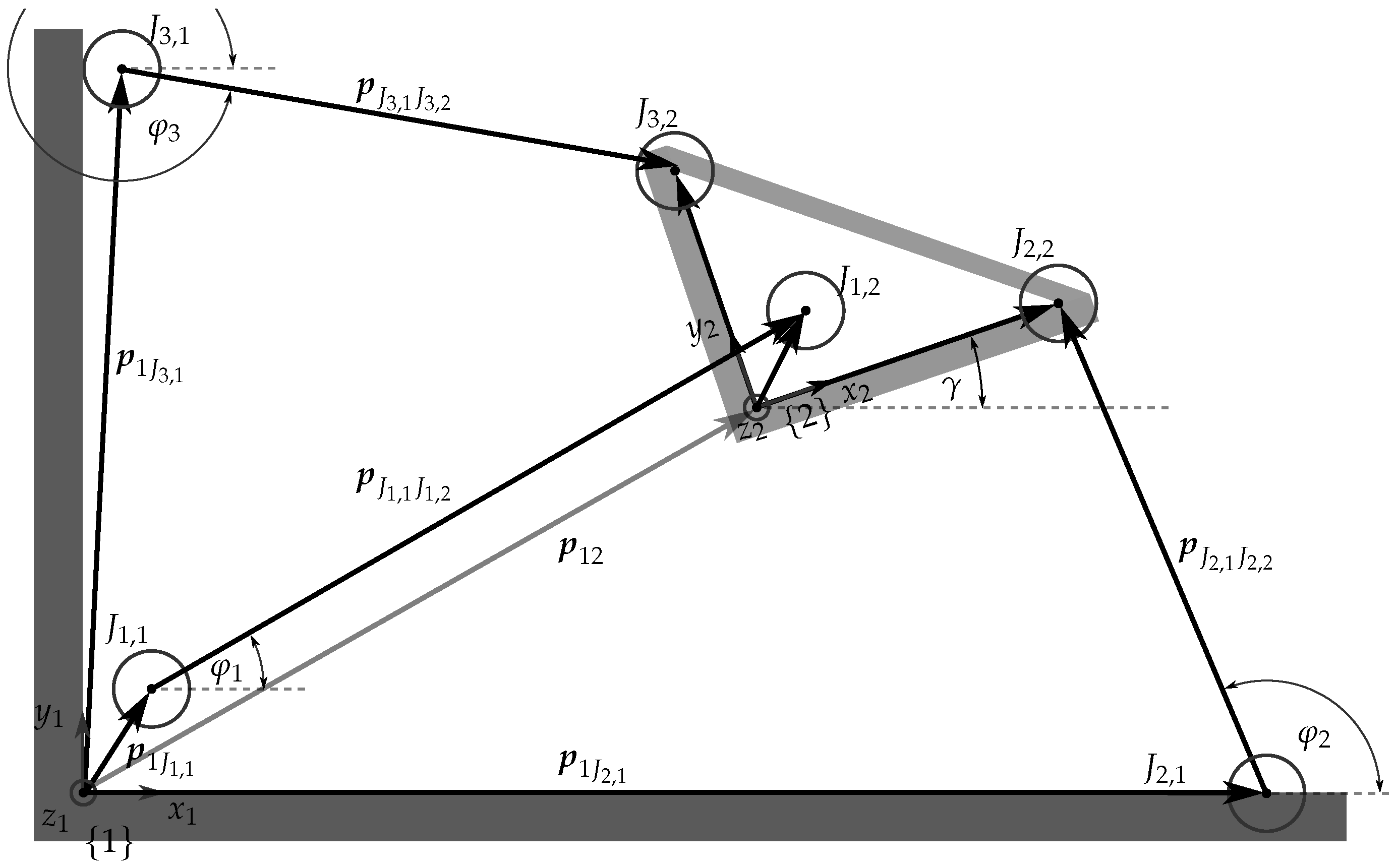
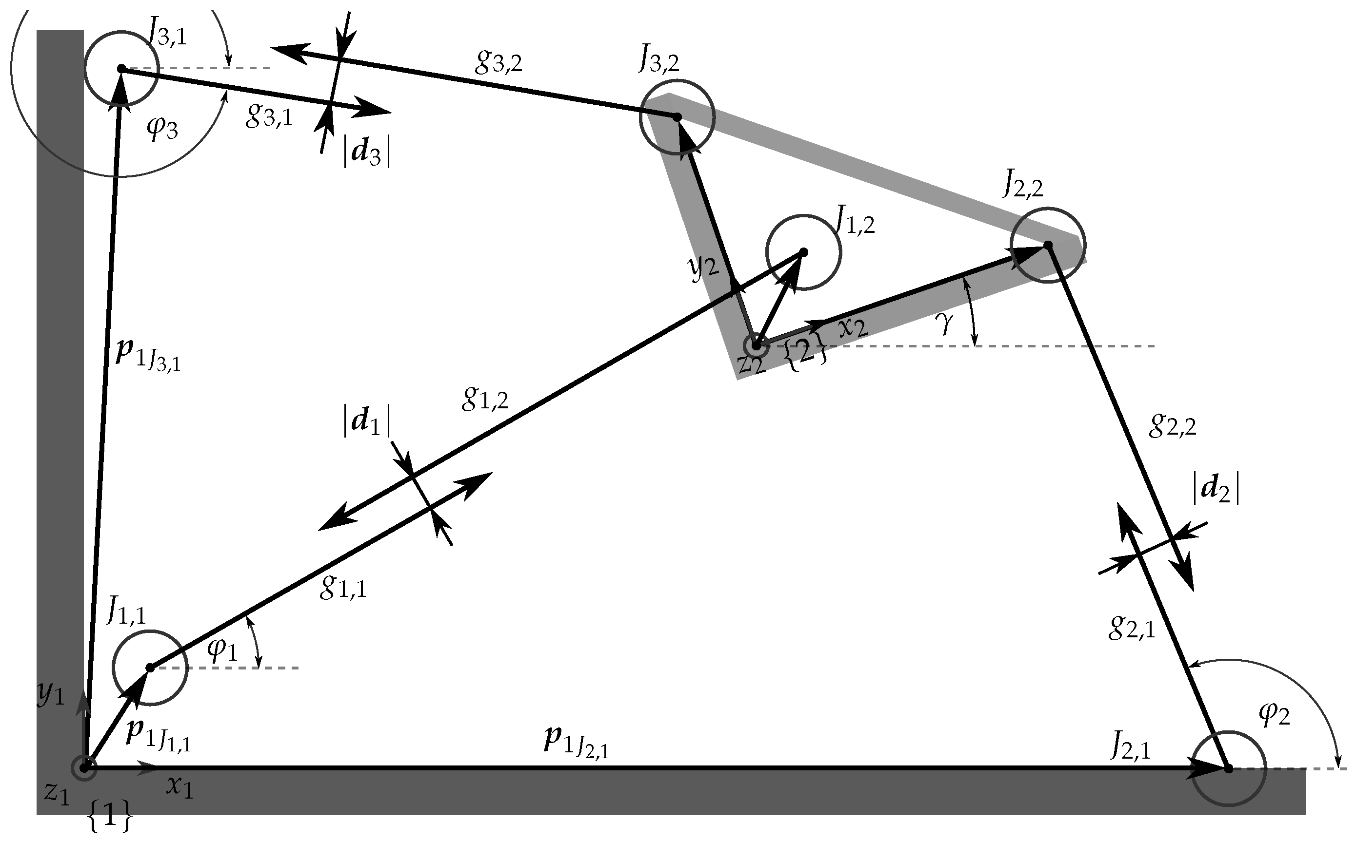
2. Direct Kinematics Solution for Planar 3-RPR Parallel Mechanisms

In this section, we present our approach for solving the direct kinematics problem of parallel mechanisms with length-variable linear actuators under dynamic conditions on the planar 3-RPR parallel mechanism. In [65], we showed that, under static conditions, it is possible to derive the manipulator platform’s pose of this mechanism only from the accelerometer values of three IMUs that are attached to two of the linear actuators as well as the manipulator platform.
The planar 3-RPR parallel mechanism consists of two platforms, a fixed base platform and a moveable manipulator platform, that are connected by three identical kinematic chains consisting of passive revolute joints on the base and the manipulator platform and, between each of them, an active prismatic joint, see Figure 1. The body-fixed coordinate system of the base platform is denoted as { 1 } and the body-fixed coordinate system of the manipulator platform as { 2 } . The planar 3-RPR parallel mechanism has two translational degrees of freedom (in the x- and y-direction) and one rotational degree of freedom (around the manipulator platform’s z-axis). With respect to the base platform { 1 } , its position is given by 1 p 12 , while its orientation is given by the rotation matrix 1 R 2 , where
1 R 2 = cos γ sin γ 0 sin γ cos γ 0 0 0 1
and γ is the rotation angle around the manipulator platform’s z-axis. The kth joint of the base platform, with k { 1 , 2 , 3 } , is denoted as J k , 1 and of the manipulator platform as J k , 2 . The vector between the joints J k , 1 and J k , 2 is given by 1 p J k , 1 , J k , 2 with respect to the base platform, while its orientation vector is referred to as 1 r J k , 1 , J k , 2 .

2.1. Robust Orientation Measurements

In a previous work [65], we obtained the orientation vector 1 r J k , 1 , J k , 2 of the kth linear actuator only from the accelerometer values of the IMUs a x , k and a y , k , where
1 r J k , 1 J k , 2 = a x , k a y , k 0 a x , k 2 + a y , k 2 .
It can also be obtained by rotating the basis vector of the base platform e x by the angle φ around the z-axis. Using the accelerometer values of the IMUs, this orientation angle φ of the kth linear actuator can be calculated as follows:
φ k , acc = atan 2 a y , a x .
However, when the linear actuators’ lengths are changed, the manipulator platform as well as the linear actuators move and the accelerometer values do not provide accurate results leading to faulty pose calculations. Robust methods for estimating the actual orientation angle φ of the linear actuators and γ of the manipulator platform thus require the IMUs’ gyroscope values ω x , ω y , and ω z in addition to the accelerometer values. It can be obtained, for example, by using a complementary filter with
φ k , com ( i ) = τ φ k φ k , com ( i 1 ) + ω k , x Δ t + ( 1 τ φ k ) φ k , acc ,
where φ k , com is the filtered orientation of the kth linear actuator, τ φ k is the ratio of gyroscope and accelerometer values, and Δ t is the time between two measurements. As an alternative, a Kalman filter can be used with
φ k , Kal ( i ) ω k , err ( i ) = 1 Δ t 0 1 φ k , Kal + ( i 1 ) ω k , err + ( i 1 ) + Δ t 0 ω k , x ( i ) , φ k , Kal + ( i ) ω k , err + ( i ) = φ k , Kal ( i ) ω k , err ( i ) + K k φ k , acc ( i ) φ k , Kal ( i ) 0 , P k ( i ) = P + ( i 1 ) + Q φ k , P k + ( i ) = P ( i ) K k S k K k ,
where φ k , Kal and φ k , Kal + are the ‘a priori’ and ‘a posteriori’ fil-tered orientations, respectively, P is the covariance estimate, S is the residual covariance, and K is the Kalman gain with
K k = P ( i ) H S k = P ( i ) 0 1 0 1 P ( i ) 0 1 + R φ k .
For the Kalman filter, the parameters of Q φ k and R φ k have to be estimated. As initial orientation estimates, both filters use the results from the accelerometer values, i. e., φ k , acc .
There are alternatives available for robustly and efficiently estimating the orientations based on IMU measurements including nonlinear complementary filters and quaternion based algorithms [67,68,69,70], but with a higher complexity.

2.2. Robust Pose Calculations

In previous works [63,64,65,66], we presented different formulations to derive the manipulator platform’s pose from the linear actuators’ orientations and the orientation of the manipulator platform. In this paper, we investigate the applicability for solving the direct kinematics problem under dynamic conditions of a method, in the following referred to as linear least-squares formulation, that uses two of the linear actuators’ orientations and the orientation of the manipulator platform and provides a unique solution with each measurement, see, for example, [65].
In the following, we review the linear least-squares formulation in a generalized form and demonstrate the possibility of sensor fusion, i. e., using all the linear actuators’ orientations together with the manipulator platform’s orientation to increase the robustness against measurement errors.

2.2.1. Linear Least-Squares Formulation

Assume that straight lines are drawn with position vectors of the base platform joints, g k , 1 , and the manipulator platform joints, g k , 2 , and orientation vectors based on the corresponding IMU values, as illustrated in Figure 2. The position vector for the kth base platform joint is given by 1 p 1 J k , 1 and for the kth manipulator platform joint by 1 p 12 + 1 R 2 · 2 p 2 J k , 2 with respect to the base platform. The position vectors for the manipulator platform joints depend on the actual position and orientation of the manipulator platform. Consider a position estimation for the manipulator platform 1 p 12 while the orientation of the manipulator platform 1 R 2 can be measured with the IMU on top of the platform. The IMUs, that are placed on the linear actuators, can measure the direction vectors from the base platform joints, r J k , 1 J k , 2 , and from the manipulator platform joints, r J k , 2 J k , 1 , where r J k , 1 J k , 2 and r J k , 2 J k , 1 point into opposite directions. Since the base and the manipulator platform joints are connected by the linear actuators, their orientation is also given by p J k , 1 J k , 2 p J k , 1 J k , 2 and p J k , 2 J k , 1 p J k , 2 J k , 1 .
Since the orientation vectors of the base and manipulator platform joints point into opposite directions, for any pose of the manipulator platform, the straight lines starting from the base platform joints, g k , 1 , are always parallel to the straight lines starting from the manipulator platform joints, g k , 2 . The distances d k between g k , 1 and g k , 2 can therefore be expressed analytically:
d k = r J k , 1 J k , 2 × 1 p 12 + 1 R 2 · 2 p 2 J k , 2 1 p 1 J k , 1 | r J k , 1 J k , 2 |
with the IMUs providing a normed direction vector
| r J k , 1 J k , 2 | = 1 ,
where d k is the distance vector between the direction vectors of the kth linear actuator, r J k , 1 J k , 2 is the direction vector of the kth linear actuator measured with the IMU, 1 p 12 is the estimated position of the manipulator platform with respect to the base, and 1 R 2 is the rotation matrix from frame { 2 } into frame { 1 } measured with the IMU.
Using the identity
a × b a ˜ · b ,
where
a = a x a y a z , a ˜ = 0 a z a y a z 0 a x a y a x 0 ,
Equation (7) can be rewritten as
d k = : b k = r ˜ J k , 1 J k , 2 · 1 p 12 + 1 R 2 · 2 p 2 J k , 2 1 p 1 J k , 1
= r ˜ J k , 1 J k , 2 = : A k · 1 p 12 = : x + r ˜ J k , 1 J k , 2 · 1 R 2 · 2 p 2 J k , 2 1 p 1 J k , 1 = : c k .
This results in an under-constrained linear least-squares problem:
A k x c k = b k , A k R 3 × 3 , x , b k , c k R 3 .
Since rank ( A k ) = 2 3 , additional information is needed to solve the linear least-squares problem distinctively. Therefore, the direction vector of a second linear actuator l is used:
A l x c l = b l .
Combining Equation (13) with Equation (14) leads to
A x c = b , A R 6 × 3 , x R 6 , b , c R 6 ,
where
A = A k A l , b = b k b l , c = c k c l .
In order to minimize b , the overdetermined linear least-squares problem in Equation (15) can be written as a minimization problem:
A x c 2 = min !
and can be reduced to a set of linear equations:
( A A = : A ¯ ) x = A c = : c ¯
with the unique solution
x = A ¯ 1 c ¯ = ( A A ) 1 A c ,
where ( A A ) 1 A is the so-called Moore-Penrose generalised inverse (for more information, see [71]). Using the found solution x , the length of the kth linear actuator can be calculated using inverse kinematics:
ρ k = ρ k , 1 = | 1 p J k , 1 J k , 2 | = | x + 1 R 2 · 2 p 2 J k , 2 1 p 1 J k , 1 | .
Therewith, a closed-form solution for the direct kinematics problem can be found with only two IMUs on the linear actuators and one IMU on the manipulator’s platform. Other algorithms for solving the linear least-squares problem are discussed in [66].

2.2.2. Sensor Fusion
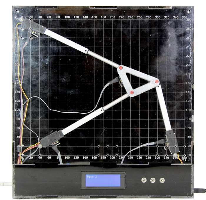
In the presence of measurement noise and other disturbances, the third linear actuator’s orientation can be used to increase the formulation’s robustness. In this context, we presented four possible sensor fusion concepts in [66] and demonstrated on the Stewart-Gough platform that therewith, the position error can be reduced by 50 %. One very elegant possibility for sensor fusion, that we will further investigate in this paper, uses the advantages of the Moore-Penrose generalized inverse. In fact, it is possible to simply add the third linear actuator’s orientation to the matrix A and the vector c leading to
A = 1 r ˜ J 1 , 1 J 1 , 2 1 r ˜ J 2 , 1 J 2 , 2 1 r ˜ J 3 , 1 J 3 , 2 R 9 × 3 ,
c = 1 r ˜ J 1 , 1 J 1 , 2 · 1 p 1 J 1 , 1 1 R 2 · 2 p 2 J 1 , 2 1 r ˜ J 2 , 1 J 2 , 2 · 1 p 1 J 2 , 1 1 R 2 · 2 p 2 J 2 , 2 1 r ˜ J 3 , 1 J 3 , 2 · 1 p 1 J 3 , 1 1 R 2 · 2 p 2 J 3 , 2 R 9 .
Due to the properties of the Moore-Penrose generalized inverse, the manipulator platform’s pose can still be found by solving Equations (18) and (19), while the solution’s robustness is significantly increased.

3. Experiment

In this section, we test our approach for solving the direct kinematics problem under dynamic conditions on a specially designed prototype of a planar 3-RPR parallel mechanism, see Figure 3. It consists of a frame, three length-variable linear actuators with integrated revolute joints at both ends, and a moveable manipulator platform. The base and manipulator platform joints’ coordinates are defined in Table 1. As linear actuators, we use Actuonix L16-100-35-P (Actuonix Motion Devices, Saanichton, BC, Canada) with a minimum length of 168 mm, a stroke length of 100 mm, and an integrated potentiometer for measuring the current length. The linear actuators and the manipulator platform are equipped with IMUs for measuring their orientations. Here, we use the accelerometer and gyroscope values of the InvenSense MPU-9250 sensors (InvenSense Inc., San Jose, CA, USA). A power supply, a display, and an Arduino Mega 2560 board (Arduino, Scarmagno, Italy) with an integrated data acquisition and pose calculation algorithm are also mounted on the frame. The Arduino Mega board is furthermore equipped with a motor shield for controlling the lengths of the linear actuators.
In the experiment, we let the manipulator platform follow a randomized trajectory for 14 s (The real-time trajectory and an extensive comparison of the orientation measurement methods and the pose calculation formulation is shown in the attached video file (Supplementary Materials)) and extract the accelerometer and gyroscope values of the IMUs as well as the linear actuators’ lengths with a sampling rate of 57.85 Hz. The measurement data are then used on a computer, first to calculate the orientations of the linear actuators and the manipulator platform’s orientation, and finally, to calculate the manipulator platform’s pose. These computations can also be done on the Arduino Mega, but this reduces the sampling rate. A comprehensive comparison of the achievable sampling rates when including the computations on the Arduino Mega is done in Section 3.1. The manipulator platform joints are equipped with small red dots that are used for optically analysing their position using image processing (the images are recorded with 60 frames per second and the resolution is 0.36 mm per pixel). Therewith, we have a ground truth of the actual manipulator platform’s pose that we can use for comparison with the results of our approach. Figure 4 shows the recorded trajectories of the manipulator platform joints. The manipulator platform’s pose is changed between 185 mm and 240 mm in the x-axis, between 145 mm and 160 mm in the y-axis, and between 10 and 46 for the platform orientation. During the experiment, the linear actuators run with velocities of ±40 mm/s.
In the following, we investigate the accuracy of both parts of the approach, the robust orientation measurement and the robust pose calculation. But first, we examine the achievable sampling rates when we include them on the Arduino Mega.

3.1. Achievable Sampling Rates

Table 2 shows the achievable sampling rates (It needs to be mentioned that the achievable sampling rate also depends on the implementation/programming of the calculations in Arduino as well as the used libraries in the code.) of the Arduino Mega when we implement different parts and formulations of our approach on the Arduino. The sampling rate is obtained as follows: The mean time between two measurements is tracked for 1000 measurements on the Arduino Mega and the result’s inverse is considered as the achievable sampling rate. It can be noticed that by solely measuring the linear actuators’ lengths, characterized by #1, the highest sampling rate (399.71 Hz) can be obtained as only the analogue inputs of the Arduino Mega board are read and multiplied by scaling factors. Measuring the IMUs’ data, characterized by #2, requires significantly more time (71.27 Hz) since a multiplexer is needed to switch between the IMUs (All the IMUs have the same address (0 × 68). In order to differentiate between them, a multiplexer is implemented that can switch the IMUs’ AD0-inputs on and off in dependence of its own input.). Including the length control into the Arduino slows down the system by another 20%. Investigating the sampling rates for the two orientation filtering concepts, it can be noticed that the complementary filter (60.41 Hz) is faster than the Kalman filter (53.02 Hz) but slower than using the raw accelerometer values (70.95 Hz). Here, we achieve higher a sampling rate compared to #4 since only five data (the four orientation angles and the Δ t ) are displayed. In this context, it needs to be mentioned that displaying data on the Arduino scope is very time consuming. Solving the linear least-squares problem on the Arduino reduces the sampling rate by another 23–34% leading to 40.82–46.20 Hz. The achievable sampling rate when using the lengths and the Newton Raphson algorithm (The Newton-Raphson algorithm used for comparison is based on the code proposed in [72].) is significantly lower (3.82 Hz).
In conclusion, although measuring orientations is significantly slower than measuring lengths (due to the need of a multiplexer to switch between the IMUs), the direct kinematics problem can still be solved considerably faster by using the proposed sensor concept. In fact, it is even possible to implement additional measurement filters to improve the formulation’s robustness and still being up to ten times faster compared to the state-of-the-art Newton Raphson algorithm. In order to increase the sampling rate, faster microcomputers such the Raspberry Pi can be used. Nevertheless, the need of a multiplexer to switch between the IMUs is immanent as all IMUs have the same address and thus remain the limiting factor.

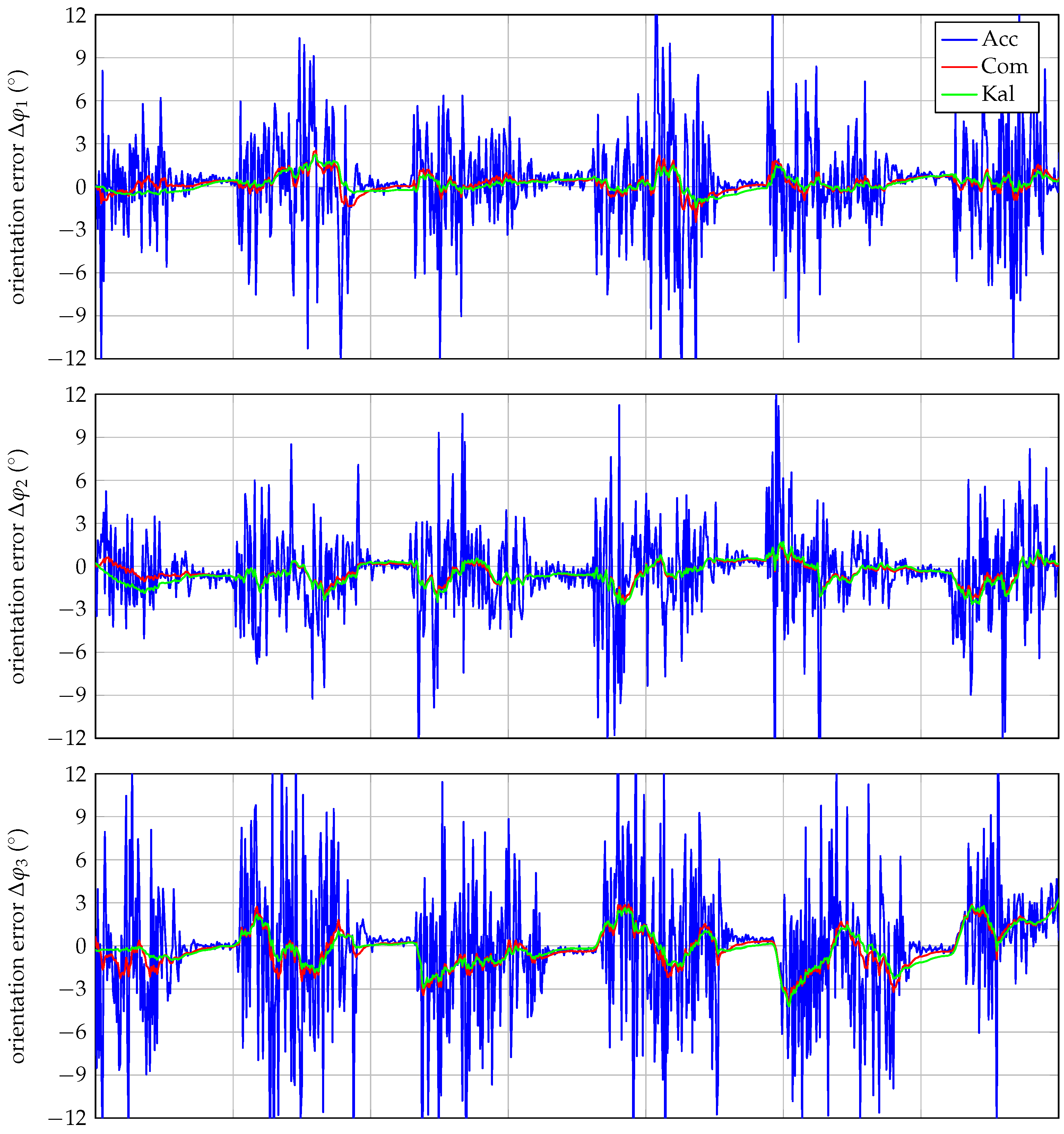
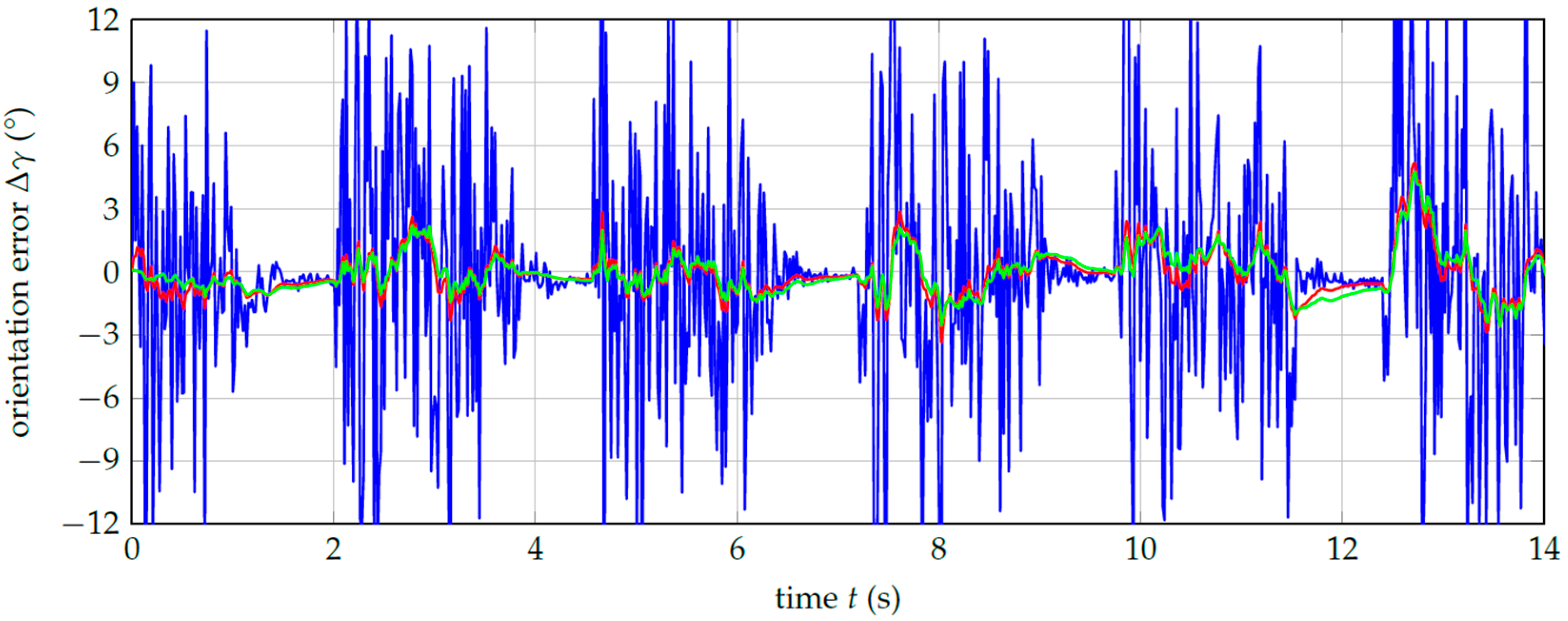
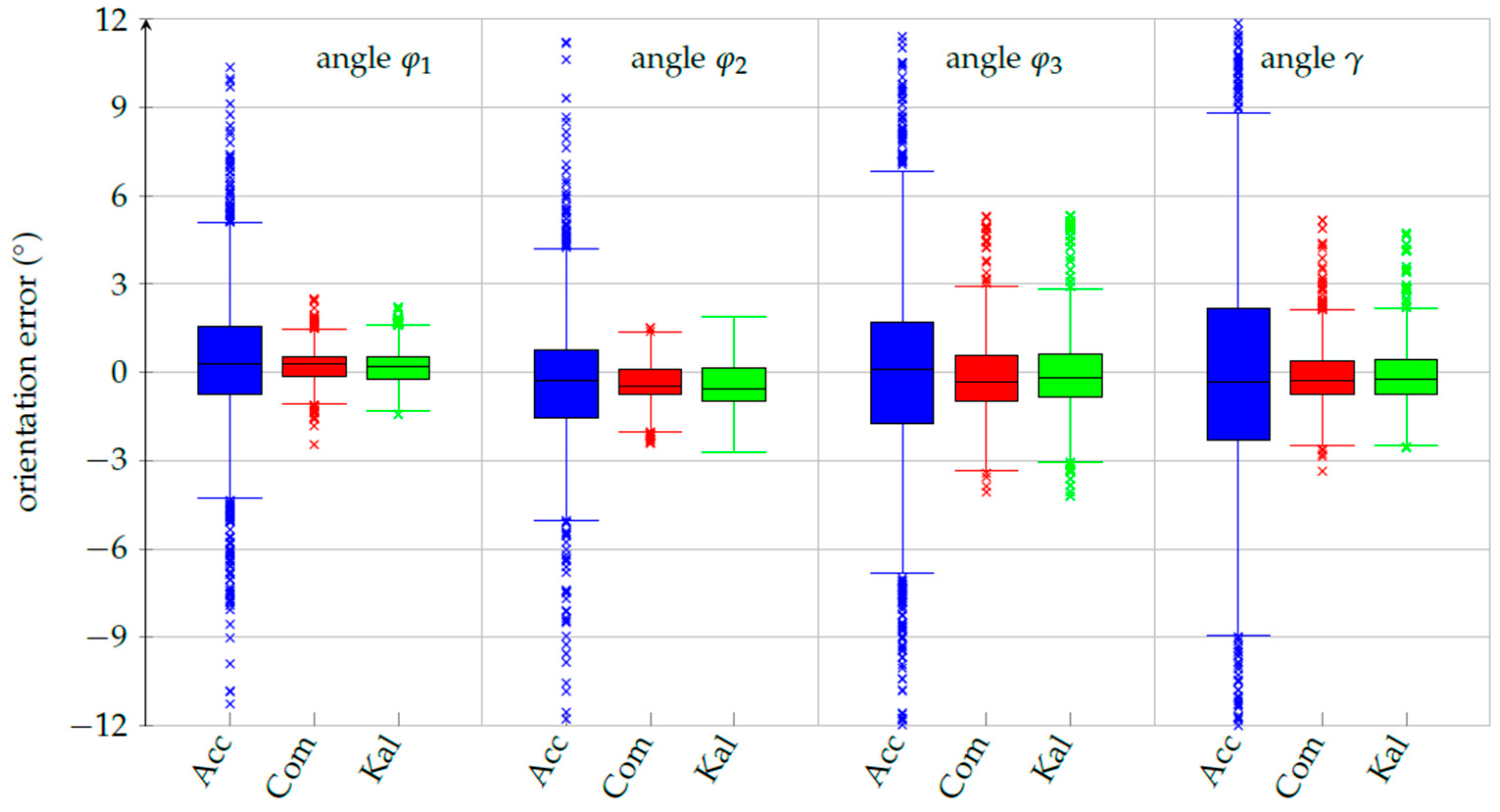
3.2. Robust Orientation Measurements

In Section 2.1, we introduced a complementary filter and a Kalman filter for robustly obtaining the orientations of the linear actuators and the manipulator platform. In this section, we compare their results with the orientations calculated from the IMUs’ raw accelerometer values and the optically derived ground truth. For the complementary filter, we use the parameters τ φ 1 = τ φ 2 = τ φ 3 = τ γ = 0 . 93 for the first, second, and third linear actuator as well as the manipulator platform. For the Kalman filter, we correspondingly use R φ 1 = R φ 3 = 3 . 75 , R φ 2 = 0 . 5 , R γ = 1 . 5 , and
Q φ 1 = Q φ 2 = Q φ 3 = Q γ = 0 . 001 0 0 0 . 005 .
These parameters were determined experimentally by minimizing the error between the measured orientations and the ground truth using a Levenberg-Marquardt algorithm.
During the trajectory shown in Figure 4, the orientation angles range between 33 and 41 for the first linear actuator, between 102 and 119 for the second linear actuator, between −21 and −33 for the third linear actuator, and between 10 and 46 for the manipulator platform. Figure 5 shows the orientation errors of the first, second, and third linear actuator as well as the manipulator platform when the orientations are calculated from the IMUs’ raw accelerometer values, the complementary filter, and the Kalman filter, respectively.
As the accelerometers of the IMUs are very sensitive, the results of the raw accelerometer values are comparatively noisy. The orientation errors range between ±6 for the first and second linear actuators’ orientations and between ±9 for the third linear actuator’s and the platform’s orientations. Due to the calibration of the IMUs, there are no offset errors. An objective comparison of the errors is given in Figure 6 where the orientation errors of the first, second, and third linear actuator as well as the manipulator platform are shown as boxplots. By using one of the introduced methods for robust orientation measurements, the orientation errors can be significantly reduced. In contrast to the raw accelerometer values that show variances between 9.15 2 (for the second linear actuator) and 32.43 2 (for the manipulator platform), the complementary filter has variances between 0.39 2 (for the first linear actuator) and 2.17 2 (for the third linear actuator). Similar results can be obtained by the Kalman filter (between 0.3 2 and 1.95 2 ).
Filtering data always introduces time delays that depend on the used filter. In fact, while the complementary filter has a time delay of one sample (17 ms) within the experiment, the Kalman filter shows a delay of 2.5 samples (42 ms). This can be traced back to the higher computational complexity.
In conclusion, both the complementary filter and the Kalman filter perform very well and remove noisy measurements. The Kalman filter shows slightly more accurate results than the complementary filter but is comparably more complex. Filtering the orientation angles is very efficient and reduces the orientation errors’ variances by 93–97%. However, orientation errors of up to ±2 for the first and second linear actuator and up to ±3 for the third linear actuator and the manipulator platform are still possible. The effect of the remaining uncertainty in the orientation measurement on accuracy of the pose calculation is investigated in the following section.

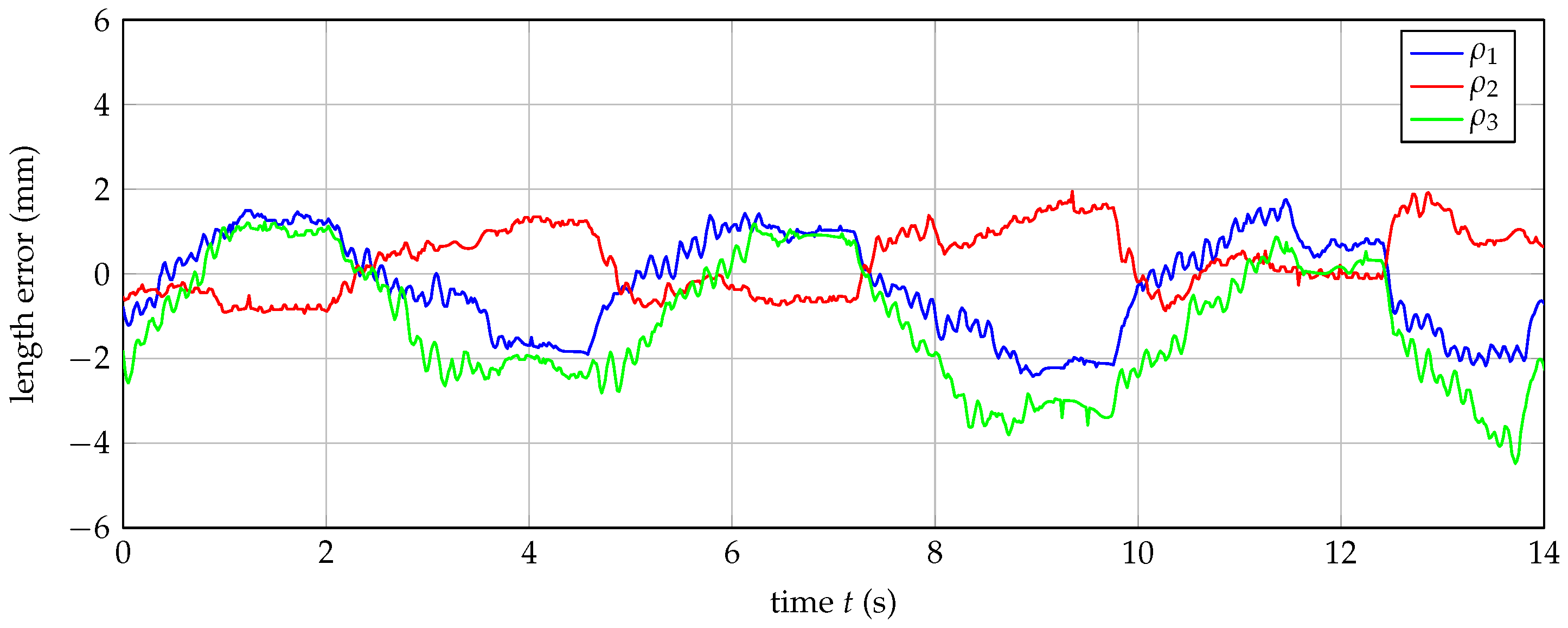
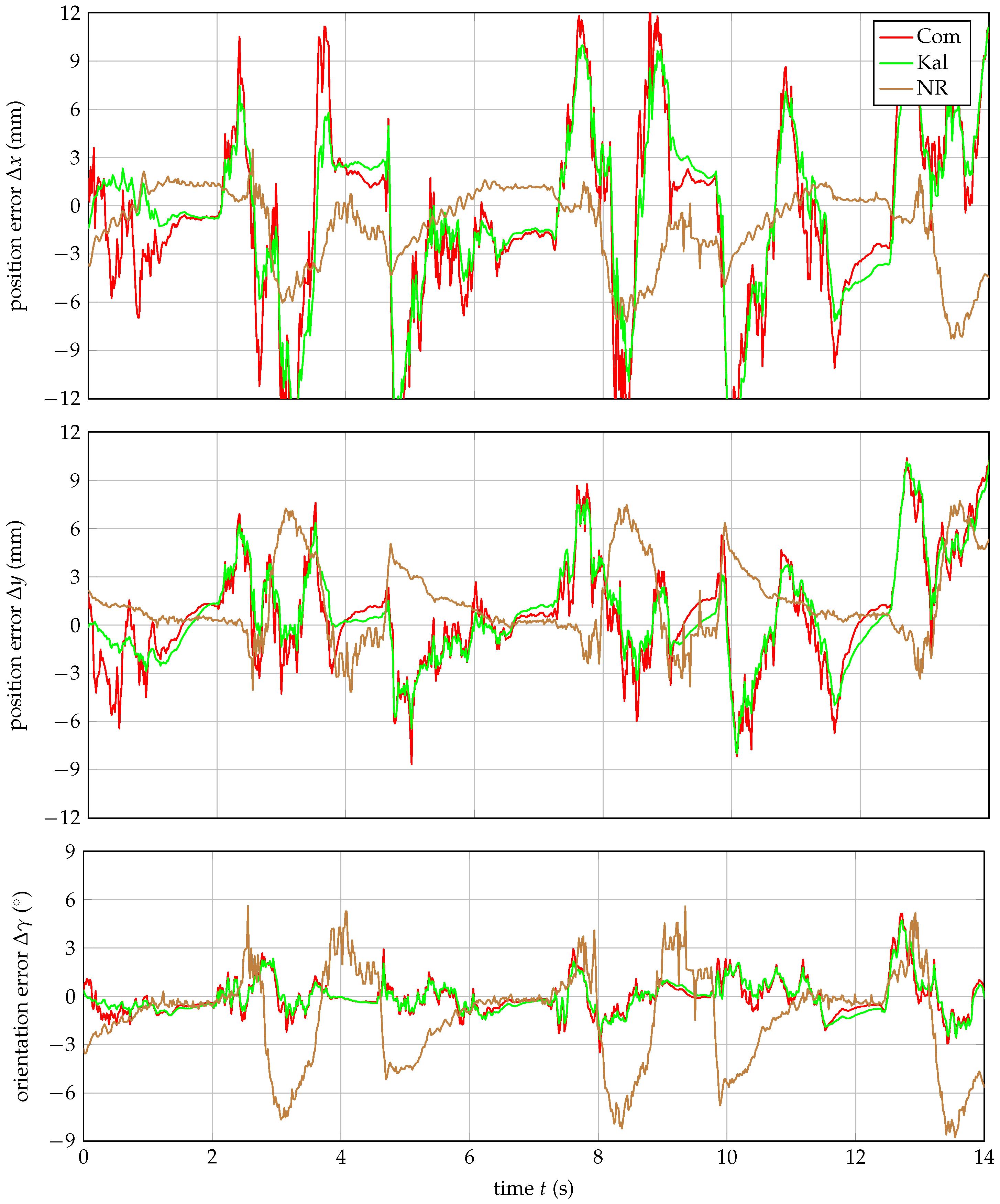
3.3. Robust Pose Calculations

In Section 2.2, we introduced the linear least-squares formulation for calculating the manipulator platform’s pose from the measured orientations of the linear actuators and the manipulator platform and demonstrated the possibility of sensor fusion to increase the solution’s robustness. In this section, we investigate the formulation’s accuracy that can be obtained when the minimum number (i. e., two) and the maximum number (i. e., three) of linear actuators’ orientations are used. As the ground truth, we use the manipulator platform’s pose that is derived optically by image processing.
In order to compare the performance of our IMU-based approach not only with the ground truth but also with a state-of-the-art method for solving the direct kinematics problem, we additionally calculate the manipulator platform’s pose from the linear actuators’ lengths using the Newton-Raphson algorithm. For the first measurement, an initial pose estimate is required. Here, we use the following initial pose estimate (This initial pose estimate allows similar results as if the actual pose is used. By using x y γ = 200 mm 150 mm 0 instead, the Newton Raphson algorithm converges to a wrong solution.):
x y γ = 230 mm 150 mm 45 .
For the following poses, we use the results of the previous measurements as initial estimates and allow three iterations between each measurement (Three iterations between each measurement is sufficient. Further iterations do not improve the results significantly.).
The linear actuators’ lengths ρ 1 ρ 3 are calculated from their potentiometer values. Due to the limited resolution of 10 bits of the Arduino Mega analog inputs, the maximum resolution of 0.0977 mm for the linear actuators’ lengths can be obtained. Figure 7 shows the error between the actual and the measured linear actuators’ lengths. Here, the actual lengths are calculated from the optically derived manipulator platform’s pose by using inverse kinematics. The linear actuators’ lengths show errors between −4 mm and 2 mm (These errors can be traced back to the uncertainties in the joints’ positions in the inverse kinematics equations due to manufacturing and assembly inaccuracies.).
Figure 8 shows the position and orientation errors during the experiment when the first and third linear actuators’ orientations and the manipulator platform orientation are used together with the proposed linear least-squares formulation. In addition, the position and orientation errors of the Newton Raphson algorithm are shown where the three linear actuators’ lengths are used. Here, only the results obtained from the filtered orientation angles are displayed. The raw orientation angles lead to significant higher position and orientation errors (±20 mm for the x- and the y-axis, and ±10 for the platform orientation). By using the filtered orientation angles instead, smaller position errors can be obtained. For example, for the x-axis, the errors mainly spread between ±9 mm. For the y-axis, even smaller position errors are obtained (between ±6 mm). The difference between the results obtained from the Kalman filtered and the complementary filtered orientation angles are comparably small (approximately less than 1 mm). The Kalman filter, however, is slightly more accurate.
Figure 9 summarises the position and orientation errors in boxplots. It can be observed that 50% of the position errors lie between ±3 mm for the x-axis and between ±2.5 mm for the y-axis while approximately 99.3% lie between ±12 mm for the x-axis and between ±8 mm for the y-axis. Figure 8 and Figure 9 also indicate that the position errors obtained from the linear actuators’ lengths and the Newton Raphson algorithm are smaller than the errors obtained with the orientations and the linear least-squares formulation. This applies particularly for the x-axis. In fact, for the Newton Raphson algorithm, 50% of the position errors lie between −3 mm and 1 mm for the x-axis and between 0 mm and 3 mm for the y-axis, while approximately 99.3% lie between −8 mm and 6 mm for the x-axis and between −4 mm and 7 mm for the y-axis. For the platform orientation, however, the Newton Raphson algorithm is less accurate than the linear least-squares formulation. In fact, while the orientation errors of the linear least-squares formulation spread between ±3 (99.3% area), the orientation errors of the Newton Raphson algorithm lie between −10 and 7 . This can be traced back to the fact that, for the linear least-squares formulation, the orientation of manipulator platform is measured, while for the Newton Raphson algorithm, the orientation is estimated from inverse kinematics and the linear actuators’ lengths. In conclusion, the linear least-squares formulation is capable of showing approximately the same accuracy as the Newton Raphson algorithm.
In Section 2.2, we additionally demonstrated the possibility of sensor fusion on the linear least-squares formulation. The results shown in Figure 8 and Figure 9 are obtained from the manipulator platform’s orientation in addition to the first and third linear actuators’ orientations. Due to the properties of the Moore-Penrose generalized inverse, we can easily add the second linear actuator’s orientation into the solution formulation to increase the robustness against measurement errors and noise without reducing the computational efficiency (i. e., reducing the sampling rate). Figure 10 shows the position and orientation errors during the experiment that are obtained when all the three linear actuators’ orientations are used. It can be observed that the position errors are significantly reduced while the orientation errors remain constant. In fact, the position error reduces by 86% for the x-axis, i. e., 50% of the position errors lie between ±1.5 mm while approximately 99.3% lie between ±5 mm. For the y-axis, sensor fusion only improves the results by 28%. For the orientation error, no improvements are obtained since no sensor fusion is done for the orientation measurement of the manipulator platform.

4. Discussion

In our experiments, the IMU-based approach for solving the direct kinematics problem of the planar 3-RPR parallel mechanism performs comparably well even under dynamic conditions. But, can the errors be further reduced when using IMUs? Is the approach generalizable, i. e., applicable to other parallel mechanisms? And, where are the limits of IMUs? In order to answer these questions, in this section, we discuss the possible application of IMUs for solving the direct kinematics problem of parallel mechanisms.
Solving the direct kinematics problem with additional sensor information is not a new idea. There are even some papers where additional orientation sensors are suggested, see, for example, [38,44]. However, none of them completely transforms the problem from length information to orientation information. In fact, the orientation sensors are always used in addition to the line actuators’ lengths. In contrast to that, our sensor concept solely uses orientation information for solving the direct kinematics problem and is, therewith, independent from any length measurement. Instead of measuring the linear actuators’ orientations by separating the two rotary degrees of freedom of the universal joints at the base platform into two consecutive revolute joints with one degree of freedom and measuring each orientation angle with a separate rotary/angular sensor, we suggested using inertial measurement units (IMUs). Those IMUs are very small, comparably cheap, and allow measuring orientations in all the axes. Among others, Merlet [73,74] used IMUs as additional orientation sensors for solving the direct kinematics problem of cable-driven parallel robots. He concluded that the IMU’s accelerometer values might be used for static pose calculations but the achievable accuracy is questionable, especially under dynamic conditions. In previous papers [63,64,65,66] and supported by this paper’s results, we came to the same conclusion. However, when using the IMU’s gyroscope in addition to the accelerometer, significantly more accurate results can be obtained. This allows to accurately calculate the manipulator platform’s pose even under dynamic conditions.
Nevertheless, IMUs have four important issues that need to be discussed when considering them for solving the direct kinematics problem of parallel mechanisms: (1) IMUs need extensive calibration and their alignment on the linear actuator needs to checked and verified. Most calibration methods require a special mechanical setup equipment to perform the calibration of the accelerometer and the gyroscope [75,76]. These are, in general, mechanical platforms that are capable of rotating the IMUs to multiple positions with known rotational velocities. As an alternative, static accelerometer calibration methods exist where the IMU is placed in several, randomly chosen positions and the parameters are derived by numerical optimization techniques [77,78,79]. (2) IMUs have a significantly lower resolution compared to an encoder on the motor’s shaft. However, they are not limited in their working range. Furthermore, in our experiment, the IMU’s resolution was even similar to the potentiometer’s resolution. (3) For measuring the rotation angle around the vertical axis, i. e., measuring the platform’s yaw angle, IMUs require additional information (magnetometer values), see, for example, [66] or iterative methods, see, for example, [69,70]. However, this will easily get quite complex, and still, the angle γ will always be more noisy and less accurate than the other angles. (4) As discovered in [66,80], the IMU’s variances depend on the linear actuator’s orientation and therefore, the position and orientation errors variances depend on them too.
In conclusion, even though IMUs have several advantages, their applicability for solving the direct kinematics problem of parallel mechanisms is questionable due to their limited resolution and the problems when measuring the rotation angle around the vertical axis. For prototypes and less complicated parallel mechanisms, IMUs can be used and provide the manipulator platform’s pose comparably accurate, unambiguously, and very fast (compared to the Newton-Raphson algorithm). For industrial applications or mechanisms where a high accuracy is required, IMUs are too noisy. As an alternative to IMUs, in the planar case, for example for the planar 3-RPR parallel mechanism, rotary encoders can be used in the revolute joints of the base platform. This would allow more accurate orientation measurements without any problems under dynamic conditions. But this would be more expensive and, for measuring the platform orientation, quite complicated. For spacial parallel mechanism, three possibilities exist for using IMUs to solve the direct kinematics problem: (1) The yaw angle of the manipulator platform is constant or can be obtained from the other angles (this applies, e. g., for the 3-RPS parallel mechanism). (2) A unique solution available without the yaw angle or even without the manipulator platform’s orientation. In fact, for the general Stewart-Gough platform, we discovered that, except for the most general case, the roll-pitch orientation of the manipulator platform together with the linear actuators’ orientations are sufficient to find a unique solution for the direct kinematics problem [64]. (3) A numerical method is implemented, for example, a Newton-Raphson algorithm or a Bayesian formulation as presented [81], where the yaw angle (or the entire platform orientation) can be estimated iteratively.

5. Conclusions

In this paper, we presented an IMU-based approach for solving the direct kinematics problem of parallel mechanisms under dynamic conditions. As an example, we applied our approach to the planar 3-RPR parallel mechanism. Here, we investigated three methods for robust orientation measurements (one that solely uses the accelerometer values, and two others that additionally use the gyroscope values together with a complementary and a Kalman filter) and compared the orientations with the actual ones that were optically analyzed using image processing. Furthermore, we revisited the linear least-squares formulation for calculating the manipulator platform’s pose from the two of the linear actuators’ orientations and the platform orientation and demonstrated the possibility of sensor fusion, i. e., using all the linear actuators’ orientations together with the orientation of the manipulator platform to increase the robustness against measurement errors. In the experiments, we let the manipulator platform follow a randomized trajectory and investigated the approach’s accuracy on our specially designed experimental planar 3-RPR parallel mechanism. Here, we compared the results with the optically analysed ground truth and those obtained from linear actuators’ lengths when the Newton-Raphson algorithm was used to compute the pose of the manipulator platform iteratively.
For the robust orientation measurement, we discovered that solely using the accelerometer values is significantly noisier than additionally using the gyroscope values. Here, the complementary filter is superior for real-time applications because it outperforms the Kalman filter in terms of complexity and shows nearly similar accuracy. For the robust pose calculation, using the raw orientation angles with the linear least-squares formulation leads to huge position and orientation errors that are too high for practical applications. By using the filtered orientation angles instead, the position and orientation errors can be significantly reduced to a range of ±9 mm and ±3 . If we furthermore introduce sensor fusion, in this case, by using all the linear actuators’ orientations, the position errors can be reduced even more. On this experimental device, they even outperform the Newton-Raphson algorithm, not only in terms of computational efficiency but also in terms of accuracy. In fact, the filtered orientations together with the linear least-squares formulation allow to find the actual pose of the manipulator platform unambiguously and independent from any initial pose estimate.
In the last section of this paper, we discussed the practical applicability of IMUs for solving the direct kinematics problem of parallel mechanisms. We concluded that IMUs can be used for prototypes and less complicated parallel mechanisms with low demands on accuracy. Here, they provide a comparably accurate, unambiguously, and very fast solution of the direct kinematics problem. Due to their limited resolution, the required calibration, and the problems when measuring the rotation angle around the vertical axis, the industrial application is questionable. However, we proposed three concepts to follow for using IMUs to solve the direct kinematics problem anyway.

Supplementary Materials

A video including the dynamic experiment, the executable Arduino code, and other information are available online at https://github.com/stefanschulz85/On-Using-Inertial-Measurement-Units-for-Solving-the-Direct-Kinematics-Problem-of-Parallel-Mechanisms (doi:10.5281/zenodo.3540813).

Funding

This research received no external funding.

Acknowledgments

Stefan Schulz would like to thank Arthur Seibel for his valuable suggestions and Abhishek Punia for his commitment during his project work. The publication of this article was supported by the Deutsche Forschungsgemeinschaft (DFG, German Research Foundation)—Projektnummer 392323616 and Hamburg University of Technology (TUHH) in the funding programme “Open Access Publishing”.

Conflicts of Interest

The author declares no conflict of interest.

References

  1. Hunt, K.H. Structural kinematics of in-parallel-actuated robot-arms. J. Mech. Transm. Autom. Des. 1983, 105, 705–712. [Google Scholar] [CrossRef]
  2. Lazard, D. Stewart platform and Gröbner basis. In Proceedings of the International Symposium on Advances in Robot Kinematics (ARK), Ferrare, Italy, 7–9 September 1992; pp. 136–142. [Google Scholar]
  3. Ronga, F.; Vust, T. Stewart platforms without computer? In Proceedings of the International Conference on Real Analytic and Algebraic Geometry, Trento, Italy, 21–25 September 1992; pp. 197–212. [Google Scholar]
  4. Lazard, D. On the representation of rigid-body motions and its application to generalized platform manipulators. In Computational Kinematics; Gladwell, G.M.L., Angeles, J., Hommel, G., Kovács, P., Eds.; Solid Mechanics and its Applications; Springer: Dordrecht, The Netherlands, 1993; Volume 28, pp. 175–181. [Google Scholar] [CrossRef]
  5. Mourrain, B. The 40 ‘generic’ positions of a parallel robot. In Proceedings of the International Symposium on Symbolic and Algebraic Computation (ISSAC), Kiev, Ukraine, 6–8 July 1993; pp. 173–182. [Google Scholar] [CrossRef]
  6. Raghavan, M. The Stewart platform of general geometry has 40 configurations. J. Mech. Des. 1993, 115, 277–282. [Google Scholar] [CrossRef]
  7. Raghavan, M.; Roth, B. Solving polynomial systems for the kinematic analysis of mechanisms and robot manipulators. ASME J. Mech. Des. 1995, 117, 71–79. [Google Scholar] [CrossRef]
  8. Husty, M.L. An algorithm for solving the direct kinematics of general Stewart-Gough platforms. Mech. Mach. Theory 1996, 31, 365–379. [Google Scholar] [CrossRef]
  9. Dietmaier, P. The Stewart-Gough platform of general geometry can have 40 real postures. In Advances in Robot Kinematics: Analysis and Control; Lenarčič, J., Husty, M.L., Eds.; Springer: Dordrecht, The Netherland, 1998; pp. 7–16. [Google Scholar] [CrossRef]
  10. Merlet, J.P. Solving the forward kinematics of a Gough-type parallel manipulator with interval analysis. Int. J. Robot. Res. 2004, 23, 221–235. [Google Scholar] [CrossRef]
  11. Porta, J.M.; Thomas, F. The forward kinematics of doubly-planar Gough-Stewart platforms and the position analysis of strips of tetrahedra. In Advances in Robot Kinematics 2018; Lenarčič, J., Parenti-Castelli, V., Eds.; Springer: Cham, Switzerland, 2019; pp. 124–132. [Google Scholar] [CrossRef]
  12. Gosselin, C.M.; Sefrioui, J.; Richard, M.J. Solutions polynomiales au problème de la cinématique directe des manipulateurs parallèles plans à trois degrés de liberté. Mech. Mach. Theory 1992, 27, 107–119. (In French) [Google Scholar] [CrossRef]
  13. Peisach, E.E. Determination of the position of the member of three-joint and two-joint four member Assur groups with rotational pairs. Machinowedenie 1985, 5, 55–61. (In Russian) [Google Scholar]
  14. Pennock, G.R.; Kassner, D.J. Kinematic analysis of a planar eight-bar linkage: Application to a platform-type robot. J. Mech. Des. 1992, 114, 87–95. [Google Scholar] [CrossRef]
  15. Wohlhart, K. Direct kinematic solution of the general planar Stewart platform. In Proceedings of the International Conference on Computer Integrated Manufacturing, Zakopane, Poland, 24–27 March 1992; pp. 403–411. [Google Scholar]
  16. Gosselin, C.; Merlet, J.P. The direct kinematics of planar parallel manipulators: Special architectures and number of solutions. Mech. Mach. Theory 1994, 29, 1083–1097. [Google Scholar] [CrossRef]
  17. Kong, X.; Gosselin, C. Forward displacement analysis of third-class analytic 3-RPR planar parallel manipulators. Mech. Mach. Theory 2001, 39, 1009–1018. [Google Scholar] [CrossRef]
  18. Collins, C.L. Forward kinematics of planar parallel manipulators in the Clifford algebra of ℙ2. Mech. Mach. Theory 2002, 37, 799–813. [Google Scholar] [CrossRef]
  19. Wenger, P.; Chablat, D. Kinematic analysis of a class of analytic planar 3-RPR parallel manipulators. In Computational Kinematics; Kecskeméthy, A., Müller, A., Eds.; Springer: Berlin, Germany, 2009; pp. 43–50. [Google Scholar] [CrossRef]
  20. Rojas, N.; Thomas, F. The forward kinematics of 3-RPR planar robots: A review and a distance-based formulation. IEEE Trans. Robot. 2011, 27, 143–150. [Google Scholar] [CrossRef]
  21. Dieudonne, J.E.; Parrish, R.V.; Bardusch, R.E. An Actuator Extension Transformation for a Motion Simulator and Inverse Transformation Applying Newton-Raphson’s Method; NASA Tech. Report TN D-7067; NASA Langley Research Center: Hampton, VA, USA, 1972.
  22. Liu, K.; Fitzgerald, J.M.; Lewis, F.L. Kinematic analysis of a Stewart platform manipulator. IEEE Trans. Ind. Electron. 1993, 40, 282–293. [Google Scholar] [CrossRef]
  23. Nguyen, C.C.; Zhou, Z.L.; Antrazi, S.S.; Campbell, C.E. Efficient Computation of Forward Kinematics and Jacobian Matrix of a Stewart Platform-Based Manipulator; IEEE of the Southeastcon: Williamsburg, VA, USA, 1991; pp. 869–874. [Google Scholar] [CrossRef]
  24. Merlet, J.P. Direct kinematics of parallel manipulator. IEEE Trans. Robot. Autom. 1993, 9, 842–846. [Google Scholar] [CrossRef]
  25. Boudreau, R.; Turkkan, N. Solving the forward kinematics of parallel manipulators with a genetic algorithm. J. Robot. Syst. 1996, 13, 111–125. [Google Scholar] [CrossRef]
  26. McAree, P.R.; Daniel, R.W. A fast, robust solution to the Stewart platform forward kinematics. J. Robot. Syst. 1996, 13, 407–427. [Google Scholar] [CrossRef]
  27. Yee, C.S.; Lim, K.B. Forward kinematics solution of Stewart platform using neural networks. Neurocomputing 1997, 16, 333–349. [Google Scholar] [CrossRef]
  28. Didrit, O.; Petitot, M.; Walter, E. Guaranteed solution of direct kinematic problems for general configurations of parallel manipulator. IEEE Trans. Robot. Autom. 1998, 14, 259–266. [Google Scholar] [CrossRef]
  29. Parikh, P.J.; Lam, S.S.Y. A hybrid strategy to solve the forward kinematics problem in parallel manipulators. IEEE Trans. Robot. 2005, 21, 18–25. [Google Scholar] [CrossRef]
  30. Liu, S.; Li, W.-L.; Du, Y.-C.; Fang, L. Forward kinematics of the Stewart platform using hybrid immune genetic algorithm. In Proceedings of the IEEE International Conference on Mechatronics and Automation, Luoyang, China, 25–28 June 2006; pp. 2330–2335. [Google Scholar] [CrossRef]
  31. Rolland, L.; Chandra, R. Forward kinematics of the 6-6 general parallel manipulator using real coded genetic algorithms. In Proceedings of the IEEE/ASME Conference on Advanced Intelligent Mechatronics (AIM), Singapore, 14–17 July 2009; pp. 1637–1642. [Google Scholar] [CrossRef]
  32. Yang, C.; Zheng, S.; Jin, J.; Zhu, S.; Han, J. Forward kinematics analysis of parallel manipulator using modified global Newton-Raphson method. J. Cent. South Univ. Technol. 1996, 17, 1264–1270. [Google Scholar] [CrossRef]
  33. Rolland, L.; Chandra, R. The forward kinematics of the 6-6 parallel manipulator using an evolutionary algorithm based on generalized generation gap with parent-centric crossover. Robotica 2016, 34, 1–22. [Google Scholar] [CrossRef]
  34. Arai, T.; Cleary, K.; Nakamura, T. Design, analysis and construction of a prototype parallel link manipulator. In Proceedings of the IEEE/RSJ International Workshop on Intelligent Robots and Systems (IROS), Ibaraki, Japan, 3–6 July 1990; pp. 205–212. [Google Scholar] [CrossRef]
  35. Shi, X.; Fenton, R.G. Forward kinematic solution of a general 6 DOF Stewart platform based on three point position data. In Proceedings of the Eighth World Congress on the Theory of Machines and Mechanism, Prague, Czechoslovakia, 26–31 August 1991; pp. 1015–1018. [Google Scholar]
  36. R. Stoughton, R.; Arai, T. Optimal sensor placement for forward kinematics evaluation of a 6-DOF parallel link manipulator. In Proceedings of the IEEE/RSJ International Workshop on Intelligent Robots and Systems (IROS), Osaka, Japan, 3–5 November 1991; pp. 785–790. [Google Scholar] [CrossRef]
  37. Cheok, K.C.; Overholt, J.L.; Beck, R.R. Exact methods for determining the kinematics of a Stewart platform using additional displacement sensors. J. Robot. Syst. 1993, 10, 689–707. [Google Scholar] [CrossRef]
  38. Merlet, J.P. Closed-form resolution of the direct kinematics of parallel manipulators using extra sensors data. In Proceedings of the IEEE International Conference on Robotics and Automation (ICRA), Atlanta, GA, USA, 2–6 May 1993; pp. 200–204. [Google Scholar] [CrossRef]
  39. Jin, Y. Exact solution for the forward kinematics of the general Stewart platform using two additional displacement sensors. In Proceedings of the 23th ASME Biennial Mechanism Conference, Minneapolis, MN, USA, 11–14 September 1994; pp. 491–945. [Google Scholar]
  40. Nair, R.; Maddocks, J.H. On the forward kinematics of parallel manipulators. Int. J. Robot. Res. 1994, 13, 171–188. [Google Scholar] [CrossRef]
  41. Etemadi-Zanganeh, K.; Angeles, J. Real-time direct kinematics of general six-degree-of-freedom parallel manipulators with minimum-sensor data. J. Robot. Syst. 1995, 12, 833–844. [Google Scholar] [CrossRef]
  42. Han, K.; Chung, W.; Youm, Y. Local structurization for the forward kinematics of parallel manipulators using extra sensor data. In Proceedings of the IEEE International Conference on Robotics and Automation (ICRA), Nagoya, Japan, 21–27 May 1995; pp. 514–520. [Google Scholar] [CrossRef]
  43. Tancredi, L.; Merlet, J.P. Extra sensors data for solving the forward kinematics problem of parallel manipulators. In Proceedings of the 9th World Congress on the Theory of Machines and Mechanisms, Milan, Italy, 29 August–2 September 1995; pp. 2122–2126. [Google Scholar]
  44. Tancredi, L.; Teillaud, M.; Merlet, J.P. Forward kinematics of a parallel manipulator with additional rotary sensors measuring the position of platform joints. In Computational Kinematics; Merlet, J.P., Ravani, B., Eds.; Solid Mechanics and its Applications; Kluwer Academic Publishers: Dordrecht, The Netherland, 1995; Volume 40, pp. 261–270. [Google Scholar] [CrossRef]
  45. Han, K.; Chung, W.; Youm, Y. New resolution scheme of the forward kinematics of parallel manipulators using extra sensor data. ASME J. Mech. Des. 1996, 118, 214–219. [Google Scholar] [CrossRef]
  46. Innocenti, C. Closed-form determination of the location of a rigid body by seven in-parallel linear transducers. J. Mech. Des. 1998, 120, 293–298. [Google Scholar] [CrossRef]
  47. Parenti-Castelli, V.; Gregorio, R.D. Real-time computation of the actual posture of the general geometry 6-6 fully-parallel mechanism using two extra rotary sensors. J. Mech. Des. 1998, 120, 549–554. [Google Scholar] [CrossRef]
  48. Bonev, I.A.; Ryu, J.; Kim, N.J.; Lee, S.K. A simple new closed-form solution of the direct kinematics of parallel manipulators using three linear extra sensors. In Proceedings of the IEEE/ASME International Conference on Advanced Intelligent Mechatronics (AIM), Atlanta, GA, USA, 19–23 September 1999; pp. 526–530. [Google Scholar] [CrossRef]
  49. Parenti-Castelli, V.; Gregorio, R.D. Determination of the actual configuration of the general Stewart platform using only one additional sensor. J. Mech. Des. 1999, 121, 21–25. [Google Scholar] [CrossRef]
  50. Baron, L.; Angeles, J. The direct kinematics of parallel manipulators under redundant sensors. IEEE Trans. Robot. Autom. 2000, 16, 12–19. [Google Scholar] [CrossRef]
  51. Baron, L.; Angeles, J. The kinematic decoupling of parallel manipulators using joint-sensor redundancy. IEEE Trans. Robot. Autom. 2000, 16, 644–651. [Google Scholar] [CrossRef]
  52. Bonev, I.A.; Ryu, J. A new method for solving the direct kinematics of general 6-6 Stewart platforms using three linear extra sensors. Mech. Mach. Theory 2000, 35, 423–436. [Google Scholar] [CrossRef]
  53. Parenti-Castelli, V.; Gregorio, R.D. A new algorithm based on two extra-sensors for real-time computation of the actual configuration of the generalized Stewart-Gough manipulator. J. Mech. Des. 2000, 122, 294–298. [Google Scholar] [CrossRef]
  54. Bonev, I.A.; Ryu, J.; Kim, N.J.; Lee, S.K. A closed-form solution to the direct kinematics of nearly general parallel manipulators with optimally located three linear extra sensors. IEEE Trans. Robot. Autom. 2001, 17, 148–156. [Google Scholar] [CrossRef]
  55. Chiu, Y.J. Forward kinematics of a general fully parallel manipulator with auxiliary sensors. Int. J. Robot. Res. 2001, 20, 401–414. [Google Scholar] [CrossRef]
  56. Vertechy, R.; Dunlop, G.R.; Parenti-Castelli, V. An accurate algorithm for the real-time solution of the direct kinematics of 6-3 Stewart platform manipulators. In Advances in Robot Kinematics; Lenarčič, J., Thomas, F., Eds.; Solid Mechanics and Its Applications; Kluwer Academic Publishers: Dordrecht, The Netherland, 2002; Volume 40, pp. 369–378. [Google Scholar] [CrossRef]
  57. Vertechy, R.; Parenti-Castelli, V. Accurate and fast body pose estimation by three point position data. Mech. Mach. Theory 2007, 42, 1170–1183. [Google Scholar] [CrossRef]
  58. Vertechy, R.; Parenti-Castelli, V. Robust, fast and accurate solution of the direct position analysis of parallel manipulators by using extra-sensors. In Parallel Manipulators, Towards New Applications; Wu, H., Ed.; I-Tech Education and Publishing: Vienna, Austria, 2008; pp. 133–154. [Google Scholar]
  59. Merlet, J.P. Parallel Robots; Springer: Dordrecht, The Netherlands, 2006. [Google Scholar] [CrossRef]
  60. Staicu, S. Power requirement comparison in the 3-RPR planar parallel robot dynamics. Mech. Mach. Theory 2009, 44, 1045–1057. [Google Scholar] [CrossRef]
  61. Chablat, D.; Jha, R.; Caro, S. A framework for the control of a parallel manipulator with several actuation modes. In Proceedings of the IEEE International Conference on Industrial Informatics (INDIN), Poitiers, France, 19–21 July 2016; pp. 190–195. [Google Scholar] [CrossRef]
  62. Moezi, S.A.; Rafeeyan, M.; Zakeri, E.; Zare, A. Simulation and experimental control of a 3-RPR parallel robot using optimal fuzzy controller and fast on/off solenoid valves based on the PWM wave. ISA Trans. 2016, 61, 265–286. [Google Scholar] [CrossRef]
  63. Schulz, S.; Seibel, A.; Schreiber, D.; Schlattmann, J. Sensor concept for solving the direct kinematics problem of the Stewart-Gough platform. In Proceedings of the IEEE/RSJ International Conference on Intelligent Robots and Systems (IROS), Vancouver, BC, Canada, 24–28 September 2017; pp. 1959–1964. [Google Scholar] [CrossRef]
  64. Seibel, A.; Schulz, S.; Schlattmann, J. On the direct kinematics problem of parallel mechanisms. J. Robot. 2018, 2018, 2412608. [Google Scholar] [CrossRef]
  65. Schulz, S.; Seibel, A.; Schlattmann, J. Closed-form solution for the direct kinematics problem of planar 3-RPR parallel mechanisms. In Proceedings of the IEEE International Conference on Robotics and Automation (ICRA), Brisbane, Australia, 21–25 May 2018; pp. 968–973. [Google Scholar] [CrossRef]
  66. Schulz, S.; Seibel, A.; Schlattmann, J. Performance of an IMU-based sensor concept for solving the direct kinematics problem of the Stewart-Gough platform. In Proceedings of the IEEE/RSJ International Conference on Intelligent Robots and Systems (IROS), Madrid, Spain, 1–5 October 2018; pp. 5055–5062. [Google Scholar] [CrossRef]
  67. Yun, X.; Lizarraga, M.; Bachmann, E.R.; McGhee, R.B. An improved quaternion-based Kalman filter for real-time tracking of rigid body orientation. In Proceedings of the IEEE/RSJ International Conference on Intelligent Robots and Systems (IROS), Las Vegas, NV, USA, 27–31 October 2003; pp. 1074–1079. [Google Scholar] [CrossRef]
  68. Mahony, R.; Hamel, T.; Pflimlin, J.M. Nonlinear complementary filters on the special orthogonal group. IEEE Trans. Autom. Control 2008, 53, 1203–1218. [Google Scholar] [CrossRef] [Green Version]
  69. Madgwick, S.O.H.; Harrison, A.J.L.; Vaidyanathan, R. Estimation of IMU and MARG orientation using a gradient descent algorithm. In Proceedings of the IEEE International Conference on Rehabilitation Robotics (ICORR), Zurich, Switzerland, 29 June–1 July 2011; pp. 179–185. [Google Scholar] [CrossRef]
  70. Valenti, R.G.; Dryanovski, I.; Xiao, J. Keeping a good attitude: A quaternion-based orientation filter for IMUs and MARGs. Sensors 2015, 15, 19302–19330. [Google Scholar] [CrossRef]
  71. Penrose, R. A generalized inverse for matrices. Math. Proc. Camb. Philos. Soc. 1955, 51, 406–413. [Google Scholar] [CrossRef] [Green Version]
  72. Press, W.H.; Teukolsky, S.A.; Vetterling, W.T.; Flannery, B.P. Numerical Recipes in C++. The Art of Scientific Computing, 2nd ed.; Cambridge University Press: Cambridge, MA, USA, 2002. [Google Scholar]
  73. Merlet, J.P. Direct kinematics of CDPR with extra cable orientation sensors: The 2 and 3 cables case with perfect measurement and sagging cables. In Proceedings of the IEEE/RSJ International Conference on Intelligent Robots and Systems (IROS), Vancouver, BC, Canada, 24–28 September 2017; pp. 6973–6978. [Google Scholar] [CrossRef] [Green Version]
  74. Merlet, J.P. An experimental investigation of extra measurements for solving the direct kinematics of cable-driven parallel robots. In Proceedings of the IEEE International Conference on Robotics and Automation (ICRA), Brisbane, Australia, 21–25 May 2018; pp. 6947–6952. [Google Scholar] [CrossRef]
  75. Nieminen, T.; Kangas, J.; Suuriniemi, S.; Kettunen, L. An enhanced multiposition calibration method for consumer grade inertial measurement units applied and tested. Meas. Sci. Technol. 2010, 21, 10. [Google Scholar] [CrossRef]
  76. Du, S.; Sun, W.; Gao, Y. MEMS IMU Error Mitigation Using Rotation Modulation Technique. Sensors 2016, 16, 2017. [Google Scholar] [CrossRef] [PubMed]
  77. Syed, Z.F.; Aggarwal, P.; Goodall, C.; Niu, X.; El-Sheimy, N. A new multi-position calibration method for MEMS inertial navigation systems. Meas. Sci. Technol. 2007, 18, 1897–1907. [Google Scholar] [CrossRef]
  78. Fong, W.T.; Ong, S.K.; Nee, A.Y.C. Methods for in-field user calibration of an inertial measurement unit without external equipment. Meas. Sci. Technol. 2008, 19, 085202. [Google Scholar] [CrossRef]
  79. Zhang, H.; Wu, Y.; Wu, W.; Wu, M.; Hu, X. Improved multi-position calibration for inertial measurement units. Meas. Sci. Technol. 2009, 21, 015107. [Google Scholar] [CrossRef]
  80. Schulz, S. Performance evaluation of a sensor concept for solving the direct kinematics problem of general planar 3-RPR parallel mechanisms by using solely the linear actuators’ orientations. Robotics 2019, 8, 72. [Google Scholar] [CrossRef] [Green Version]
  81. Schulz, S.; Seibel, A.; Schlattmann, J. Solution for the direct kinematics problem of the general Stewart-Gough Platform by using only linear actuators’ orientations. In Advances in Robot Kinematics 2018; Lenarčič, J., Parenti-Castelli, V., Eds.; Springer: Cham, Swizerland, 2019; pp. 124–132. [Google Scholar] [CrossRef]
Figure 1. Planar 3-RPR parallel mechanism with three linear actuators, three base platform joints, and three manipulator platform joints.
Robotics 08 00099 g001
Figure 2. Schematic diagram of the linear least-squares formulation for solving the direct kinematics problem of the planar 3-RPR parallel mechanism.
Robotics 08 00099 g002
Figure 3. Specially designed prototype of a planar 3-RPR parallel mechanism. Actuonix L16-100-35-P linear actuators are used with a minimum length of 168 mm and a stroke length of 100 mm. As IMUs, InvenSense MPU-9250 sensors are chosen and mounted on the linear actuators as well as the manipulator platform. The device also consists of a power supply, a display, an Arduino Mega board with a data acquisition and pose calculation algorithm, and a motor shield for controlling the linear actuators’ lengths.
Robotics 08 00099 g003
Figure 4. Trajectories of the first (blue), second (red), and third (green) manipulator platform joint during the experiments. The trajectory is recorded by a camera, and the joints’ positions are analyzed using image processing.
Robotics 08 00099 g004
Figure 5. Orientation errors of the first linear actuator, the second linear actuator, the third linear actuator, and the manipulator platform. The orientation angles are obtained from the accelerometer values (blue), the complementary filter (red), and the Kalman filter (green). As reference, the orientations calculated from the optically analyzed manipulator platform joints are used.
Robotics 08 00099 g005aRobotics 08 00099 g005b
Figure 6. Boxplots of the orientation errors of the first linear actuator, the third linear actuator, and the manipulator platform obtained from the accelerometer values, the complementary filter, and the Kalman filter, respectively. The box corresponds to the area in which the middle 50% of the errors lie while the whiskers indicate the area in which the middle 99.3% of the errors lie.
Robotics 08 00099 g006
Figure 7. Lengths errors of the first, second, and third linear actuator. The lengths are calculated from the linear actuators’ potentiometer values and compared with the actual lengths that are calculated from the optically derived manipulator platform’s pose by using inverse kinematics.
Robotics 08 00099 g007
Figure 8. Position and orientation errors of the manipulator platform’s pose calculated with the linear least-squares formulation and the filtered first and third linear actuators’ orientations. In addition, the position and orientation errors of the manipulator platform’s pose calculated with the linear actuators’ lengths and the Newton Raphson algorithm are shown. As ground truth, in both cases, the positions and orientations calculated from the optically analyzed manipulator platform joints are used.
Robotics 08 00099 g008
Figure 9. Boxplots of the position and orientation errors of the manipulator platform’s pose during the experiment calculated with the linear least-squares formulation and the filtered first and third linear actuators’ orientations. In addition, boxplots of the position and orientation errors of the manipulator platform’s pose calculated with the linear actuators’ lengths and the Newton Raphson algorithm are shown. As ground truth, in both cases, the positions and orientations calculated from the optically analyzed manipulator platform joints are used. The box corresponds to the area in which the middle 50% of the errors lie while the whiskers indicate the area in which the middle 99.3% of the errors lie.
Robotics 08 00099 g009
Figure 10. Position and orientation errors of the manipulator platform’s pose calculated with the linear least-squares formulation and the filtered first, second, and third linear actuators’ orientations. As ground truth, in both cases, the positions and orientations calculated from the optically analyzed manipulator platform joints are used.
Robotics 08 00099 g010
Table 1. Coordinates of the base and manipulator platform joints. All unit s are in mm.
Base Platform JointsManipulator Platform Joints
1 p 1 J 1 , 1 1 p 1 J 2 , 1 1 p 1 J 3 , 1 2 p 2 J 1 , 2 2 p 2 J 2 , 2 2 p 2 J 3 , 2
40 20 0 340 0 0 0 300 0 0 0 0 60 0 0 0 60 0
Table 2. Achievable sampling rates of the Arduino Mega depending on the calculations contained and the displayed data. The sampling rates are considered as the inverse of the mean time between two measurements evaluated over 1000 measurements.
No.Included CalculationDisplayed DataSampling Rate
1length measurement (3 lengths)4399.71 Hz
2orientation measurement (4 IMUs)1671.27 Hz
3#1 + length control4293.88 Hz
4#1 + #2 + length control1657.85 Hz
5a#4 + raw angles570.95 Hz
5b#4 + orientation filtering (complementary filter)560.41 Hz
5c#4 + orientation filtering (Kalman filter)553.02 Hz
6a#5a + linear least-squares formulation446.20 Hz
6b#5b + linear least-squares formulation444.82 Hz
6c#5c + linear least-squares formulation440.82 Hz
7#3 + Newton Raphson algorithm43.82 Hz

