Estimating Weight of Unknown Objects Using Active Thermography

Abstract

Successful manipulation of unknown objects requires an understanding of their physical properties. Infrared thermography has the potential to provide real-time, contactless material characterization for unknown objects. In this paper, we propose an approach that utilizes active thermography and custom multi-channel neural networks to perform classification between samples and regression towards the density property. With the help of an off-the-shelf technology to estimate the volume of the object, the proposed approach is capable of estimating the weight of the unknown object. We show the efficacy of the infrared thermography approach to a set of ten commonly used materials to achieve a 99.1% R²-fit for predicted versus actual density values. The system can be used with tele-operated or autonomous robots to optimize grasping techniques for unknown objects without touching them.

1. Introduction

As robots make their way into real-world applications such as in construction, manufacturing, human interaction, and other civilian and military applications in the marina, aerial or space arena, there is an increasing demand for physical interaction with unknown environments [1]. In a typical manipulation task, the robot is required to develop a gripping technique based on the physical properties of the object. For successful manipulation, suitable grasping forces have to be determined preferably before making any physical contact with the object. If the applied force is not sufficient, then the object can slip, whereas too much force may damage the object. One of the standing problems endured in grasping unknown objects is the lack of real-time information about the weight of unknown objects without touching or lifting them.

Inspired by the fact that humans use rough weight guesses from vision as initial estimation, followed by tactile afferent control that improves the grasping precision, a common technique for estimating object weight is the execution of prevision grips [2]. Weight estimation involves five steps: initial positioning of the robotic arm around the object, (2) grasping and lifting the object, (3) unsupported holding of the object, (4) returning the object to its initial position, and (5) returning the robotic arm to its initial position [3]. The weight of the object is estimated as the difference between the forces exerted by the robotic arm in steps (2) and (3) along the three directions of motion (change in the load force is due to gravity). A fundamental limitation of this approach is the need to make contact before knowing the physical properties of the object.

Active thermography is a remote and non-contact method with the potential to examine the physical properties of objects in unknown environments, such as material classification [4] or thermal characterization [5]. This approach relies on shining a laser source at the surface of the object, uses a thermal camera to examine the dissipation of thermal heat at the surface of the object, and feeds the thermal stream into a machine learning classifier or regressor to identify the material class of the object or to estimate its corresponding physical properties. In this paper, we present an approach to estimate the weight of an unknown object by estimating the density of the object using active thermography and estimating its the volume. The approach feeds the thermal signatures into a custom multi-channel neural network to estimate the density of the object and combines it with the volume measurement to estimate the weight of the object.

In a real-world application, the Haptic Eye system would be mounted on a robotic system. Whenever the robot intends to physically manipulate with an unknown object, it activates the Haptic Eye system to estimate the physical properties of the object before touching it. The robot may tailor its approach for physical interaction with the unknown object accordingly. An interesting scenario is that, when the robot intends to lift the unknown object, it needs to know about its weight to optimize the grasping task.

Heat transfer principles, described using the heat equation, suggest that the rate at which the material at a point will heat up (or cool down) is proportional to how much hotter (or cooler) the surrounding material is [6]. The thermal diffusivity is dependent on the thermal conductivity, the specific heat, and the density of the material. Therefore, the proposed approach capitalizes on such a relationship to estimate density of material by observing the corresponding thermal properties. The contributions of this paper include the following:

• A proposal for the weight estimation framework for physical interaction with unknown objects.
• A realization of the proposed framework using a multi-channel neural network.
• Experimental validation and testing of its characterization functionality with results that improve on the state of the art.

The rest of this paper is organized as follows: Section 2 gives an overview of the existing approaches for weight estimation. Section 3 contains a conceptual presentation of our approach, including a description of the weight estimation framework. A realization of this framework is described in Section 4, including density estimation, volume estimation, and the results. The findings as well as the limitations of the proposed approach are discussed in Section 5. Finally, conclusions are drawn in Section 6, along with stating our future directions for research.

2. Related Work

Recent developments in computer vision and machine learning have opened the door to explore the possibility of estimating the weight of an object using visual information obtained from 2D or 3D cameras. Weight estimation for specific materials is already explored, such as detecting the weight of Alaskan salmon [7], beef [8], pigs [9], and human body parts [10]. A broader list of food classes such as banana or bread are considered for computing the mass in [11]. The system solves a classification problem to find out the material type and looks up a pre-measured density for that object material as an estimate of the object’s density. A similar method used videos of simple platonic solids with an object tracker and a physical simulator to learn parameters of the simulator, including the mass of the object [12]. Another interesting work created a large-scale dataset containing both the images of objects and their mass information that is easily available [13]. The system used the 2D image of the object to estimate its weight. Results demonstrated that the proposed model performed significantly better than humans (to estimate weight of familiar objects). However, an unresolved challenge is the ability to estimate the weight of objects which the system has not been trained for.

Inspired by how humans estimate the weight of unknown objects by unsupported holding, a fundamentally different approach involves a robotic arm performing a precision grip of the object to estimate its weight [14]. The robotic arm is equipped with tactile sensors for slip detection and to measure contact forces during object manipulation (holding). Recent advances in tactile sensing technologies such as BioTac [15], OptoForce [16] and the skinline magnetic-based technology [17] boosted this approach. In a recent work [18], a robotic gripper is used to estimate a target object’s geometric information and center of mass using 3D soft force sensors. Results demonstrated the ability of the system to discriminate objects that have identical external properties but different mass distributions. The authors in [3] presented a manipulation action of power grasp with an online estimation of object weight within a very short time (0.5–0.7 s), in the absence of friction interaction between the object and the grasping arm. In a subsequent work [19], the weight of the object is estimated from currents flowing in motor servos where results showed successful estimation of the weight of the object with a 22% average error. A method is also presented in [14] for estimating the mass of an object using a precision grip on a humanoid robot. A recent research work presented a method to estimate the weight of an object during a precision grip made by a humanoid robot where tactile sensors on the fingertips provide 3D force information during a movement of grasping and lifting a cup filled with different masses, with static and dynamic friction taken into consideration [20]. The system is able to calculate the object weight for eight different masses, with satisfactory performance. This approach is challenged by several factors. First, of all, weight perception with humans is not always reliable, due to a phenomenon known as weight illusion [21], caused by the object’s size and material. Furthermore, the approach requires physical contact before learning about the weight of the object, which increases the chances of slippage (the state of the art reports an 80% success rate for detecting slip, which is not good enough for many applications).

An emerging, interesting approach is to use active thermography for material characterization [4,5]. A model-based approach for characterizing unknown materials using laser thermography is proposed in [4]. Results demonstrated the ability of the approach to classify different materials based on their thermal properties. In a subsequent work [5], an approach is proposed to combine infrared thermography with machine learning for a fast, accurate classification of objects with different material composition. Results showed that a classification accuracy of around 97% can be achieved with majority vote decision tree classification. In this paper, we aim to extend this approach for classification and regression in order to estimate the density of the material based on thermal signature and an off-the-shelf volume estimation technique to estimate the weight of an unknown object using convolutional neural networks.

3. Weight Estimation Framework

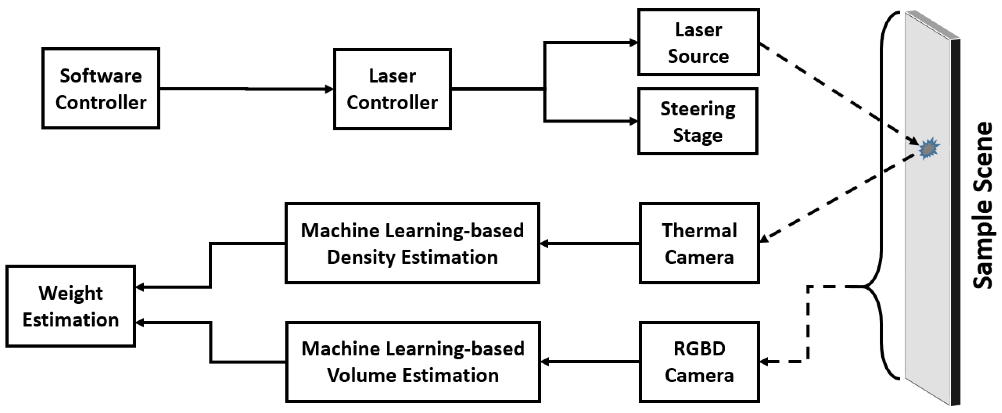
The proposed approach is depicted in Figure 1, and it consists of two processes working in parallel: volume estimation and density estimation. Volume estimation may rely on off-the-shelf techniques to contactlessly measure the volume of a sample. Existing methods, such as [22], can be applied to measure the volume of unknown samples. This is considered beyond the scope of this research and thus the current study focuses on estimating the density of the sampled material.

The density estimation is done by using an infrared thermography setup. A Software Controller is responsible for initiating the procedure and delivering the detailed instructions to the Laser Controller, which in turn supplies control input (excitation timing, duration, shape, waveform, etc.) to the Laser Source and the optional Steering Stage, which can be used if a scanning motion over a multitude of excitation locations is carried out. The excitation provided by the Laser Source component hits the surface of the Sample and results in heating it up by a minuscule amount. This creates a thermal gradient over the surface of the sample around the excitation location, and it evolves over time in a way that depends on the thermal properties of the material. The Thermal Camera captures this process in a series of radiometric or thermal frames and passes them onto the next stage, where these data are processed and fed into a machine learning algorithm. The output of this component is an estimate on the density of the material. This is then combined with the output of the volume estimation component to yield a weight estimate.

4. Experimental Realization

This section details how the components of the Weight Estimation Framework can be realized.

4.1. Sample Material Set

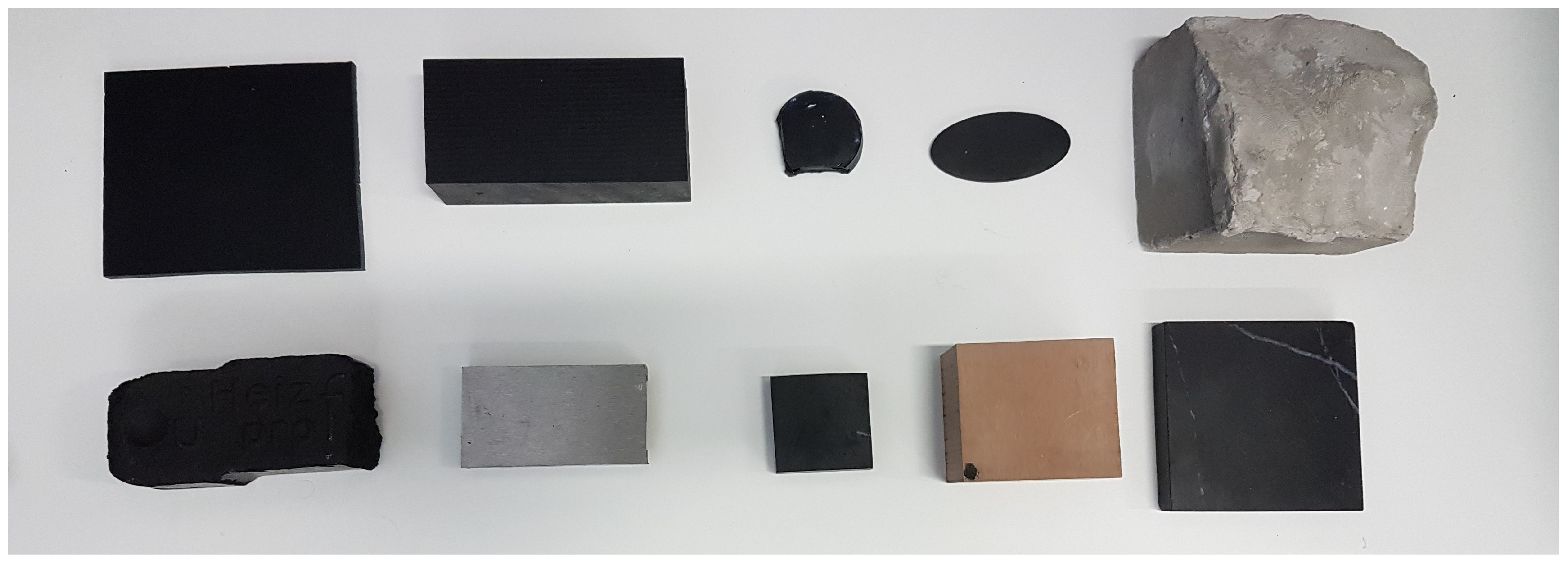
The literature about material science reports four families of physical material: polymers, ceramics, metals, and composites [23]. A sample set of 10 materials is designed with three selection criteria: (1) samples must represent the four families of material, (2) samples entail a large range of thermal properties (thermal conductivity, diffusivity, and effusivity ranges), and (3) samples are highly available in every day’s life. Based on these criteria, five polymer samples are selected, namely, silicone, acrylic glass, sorbothane, polyethylene, and coal (as a polymer composite). Similarly, two composite material samples are considered, namely low pressure laminate and high pressure laminate. Concrete and marble (as ceramic composites) are going to represent the ceramic family. Finally, steel is included as a widely available metal. A snapshot of these samples is shown in Figure 2. Note that these samples are also selected with variations in size, shape, and weight properties in order to examine the robustness of the proposed approach and thus the suitability for real-world applications.

4.2. Density Estimation

4.2.1. Experimental Setup

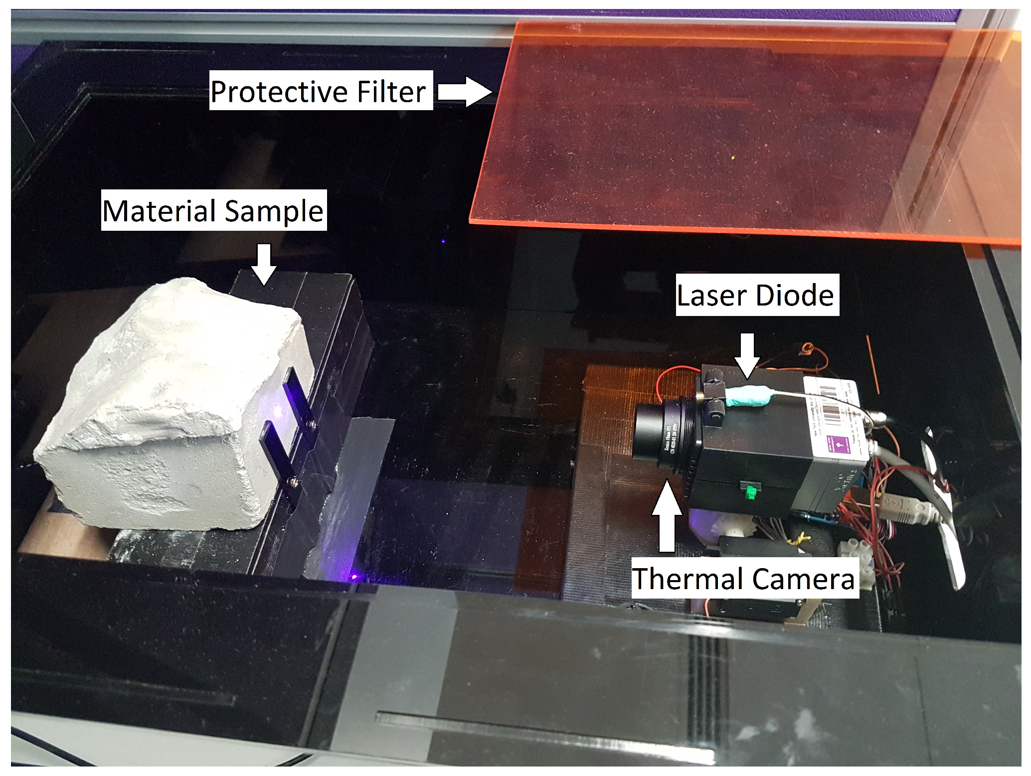
The experimental setup consisted of the following elements: a US-Lasers Inc. D405-120 laser diode (La Puente, California, USA) with a wavelength of 405 nm and an operating power of 120 mW performed the excitation on the sample object, and a Xenics Gobi-640-GigE thermal camera (Leuven, Belgium) was responsible for recording the data in radiometric mode. The camera works in the longwave infrared range (LWIR), which corresponds to the 8–14 μm wavelength range. Its Noise Equivalent Temperature Difference (NETD) in thermographic mode is rated to be not more than 50 mK. The camera was located 19.5 cm away from the sample, while the laser diode was a further 3 cm behind it. Figure 3 shows this active thermography setup with the concrete sample in place.

The recorded footage had a resolution of 640 pixels across the width and 480 pixels high with a frame rate of 50 Hz, where the individual pixels represent the radiometric measurements on the corresponding locations of the surface of the object on a 16-bit scale. An Arduino board was responsible for controlling a relay that turns the laser on and off. This board was connected to a desktop PC and was controlled through a serial connection, while the camera was connected to the PC through Gigabit Ethernet for control of the recording process and acquiring the recorded data. The PC ran a script in MATLAB R2018a that simultaneously controlled the Arduino board and the thermal camera to ensure these elements are synchronized throughout the data acquisition process. A total of 10 different samples were used for this experiment. These are listed in

Table 1. List of samples and their normalized physical properties.

Sample	Weight (g)	Volume (cm3)	Density (g/cm3)
Concrete	545	380	1.43
Polyethylene (PE)	535	380	1.41
Acrylic	132	113	1.17
Coal	130	105	1.24
Marble	516	298	2.61
Sorbothane	13.7	16	0.86
Low-Pressure Laminate (LPL)	191	281	0.68
High-Pressure Laminate (HPL)	60	43	1.40
Steel	372	48	7.75
Silicone	14.0	10	1.40

and shown in Figure 2.

4.2.2. Data Acquisition and Processing

The data acquisition consisted of two parts: acquiring the predictor data (radiometric frames and time stamps) and the target data (density values).

The predictor data acquisition took place in a set of 10 successive sessions over 10 days. Each session consisted of 10 experimental rounds for a certain sample, then the same 10 rounds for the next sample, and so on. An experimental round contained the following steps: first, the camera records 40 frames without any laser excitation. These frames were used later in the processing phase to remove the ambient component of the signal. Once these frames are recorded, the laser diode turns on for 5 s to provide the excitation. As soon as this time is over, the laser diode turns off and simultaneously the camera begins to record a series of 100 frames, which act as the signal part. Given the 50 Hz frame rate of the camera, this process takes less than 8 s, and it is followed by a timeout of 2 min before the next round takes place to avoid any interference between the excitation of subsequent rounds.

The target data acquisition involved determining the density values of each of the samples. Measuring the weight of each samples was conducted with scales, while measuring the volume involved measuring the dimensionality of rectangular samples, cutting the non-rectangular samples into rectangular shape (normalization) or using measuring tubes to determine their volumes based on the change in water level in the tube before and after they are fully submerged. The acquired values are visible in Table 1. It can be noted that concrete, polyethylene (PE), TRESPA (HPL) and silicone samples had density values that are very close to each other. On the one hand, this meant to challenge the network to predict a similar value for each of these different materials while others have markedly different values. On the other hand, it also served as an illustration to real world conditions where seemingly different materials can have similar densities.

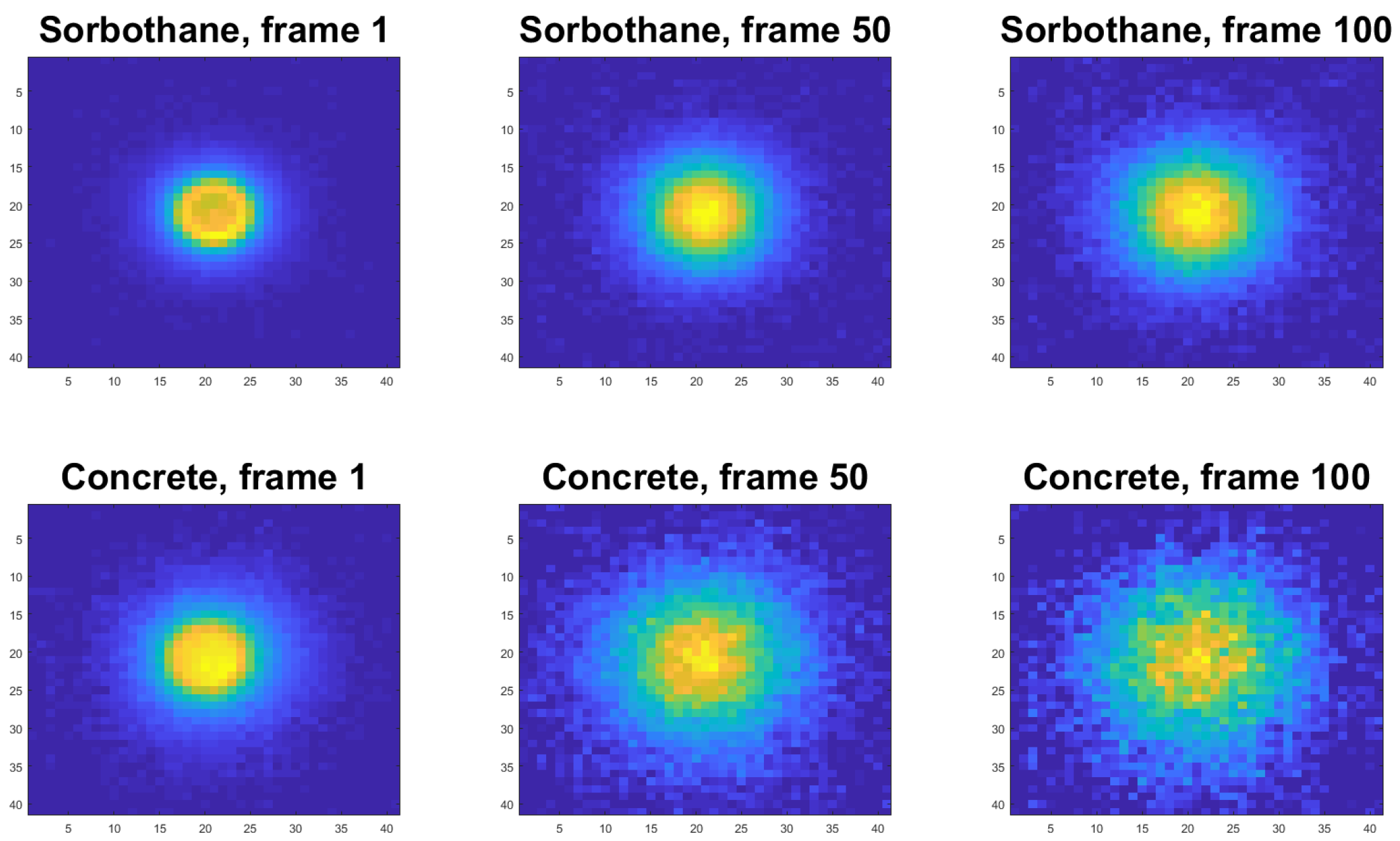
The radiometric data are processed in several steps being used as the input to the neural network. This includes, for each experimental round, using the average of the 40 pre-excitation frames and subtracting it from each of the 100 frames recorded after the excitation. This ensures that the system can be more robust with respect to changes in the ambient temperature. These frames are also cropped to a resolution of 320 pixels in width and 240 pixels in height containing the excitation region so even if the sample is relatively small, its background will not distort the signal. Finally, the center of the excitation is determined based on a smoothed average of the first 10 frames, and the frames are cropped to the 41 pixels of width and 41 pixels of height region of this point.

Figure 4 demonstrates visually, using an example of three frames in the same experimental round, how the thermal dissipation is varying depending on the material properties of the sample. Note that the increase in temperature varied between the samples as it is dependent on the material’s thermal effusivity, but this temperature change never exceeded more than two degrees for any of the samples.

4.2.3. Neural Network Design and Training

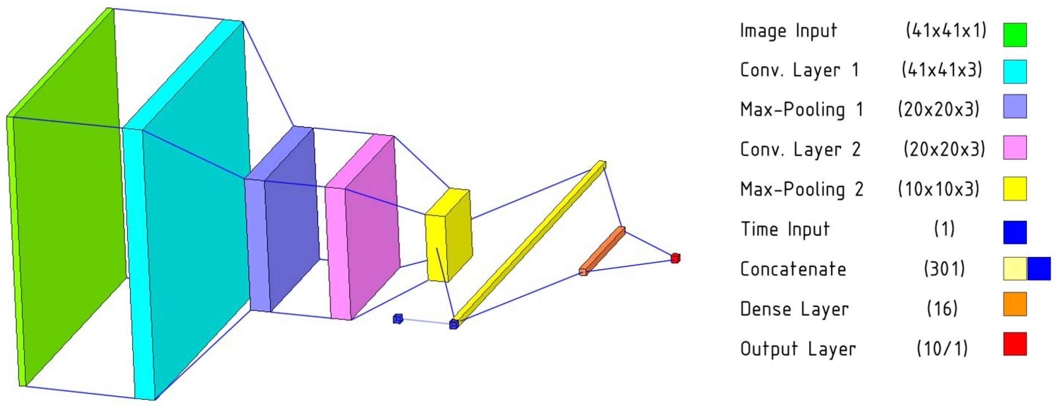
When designing the neural network to perform regression on the radiometric frames to the density values, it was essential to abide by the limitations posed by the size of the data set, yet take advantage of all the information that the system can rely on. Using an entire recording as data for a single density value would have meant that our entire data set has a size of 1000, which is not enough to train a neural network. Therefore, we have decided to examine if the network is capable of predicting the density from a single thermal frame. This meant our data set size is the total number of frames, which is 100,000. This was enough to train a shallow convolutional neural network. Having tried various designs, we have arrived at a network that takes the individual frames with 41 pixels width by 41 pixels height resolution and puts them through two convolutional stages. Both of these convolutional stages consist of a convolutional layer with a 3-by-3 kernel and 3 output channels, a max-pooling layer with 2-by-2 size and a stride of 1, and a batch normalization layer. These are followed by a fully connected stage consisting of a fully connected layer with 16 hidden units, and an output layer with a single unit that is supposed to be the numerical value expressing the density in g/cm³. All layers before the output layer rely on sigmoid activation.

Given that we ended up using the individual frames as separate data points, it can be a challenge for the network to correctly equate the first and the last image of the same recording and predict identical (or near-identical) values for them, given that they are captured when different amounts of time have passed since the end of the excitation. In order to overcome this challenge, we added an auxiliary scalar input to the network, in parallel to the convolutional stages. This input carries the value of the frame number (1 to 100 according to its location in its recording) and helps the network counteract the possible discrepancy between different time delays between the end of excitation and the capturing of the frames. This auxiliary input is concatenated to the flattened output of the second convolutional stage and these together serve as the input for the network. The final multi-channel neural network has 5577 trainable parameters and its structure is visible in Figure 5. In order to evaluate the suitability of this network, we have devised two other regressors for comparison. The “baseline 1” network lacks the auxiliary time input but is otherwise identical to the multi-channel neural network. The “baseline 2” network is an ordinary linear regression model that uses each pixel as separate predictors.

When training the network, the data set was partitioned into three sets: training set, validation set and testing set. In addition to these sets being completely disjoint, it was essential to ensure that frames from the same recordings did not appear in more than one set. This would compromise the learning process as the network could be inclined to exploit similarities in subsequent frames in the different sets instead of being forced to learn meaningful features that are robust to different recordings. It was therefore decided to separate the data based on data acquisition sessions. The training set is made up of eight sessions (80 rounds per material sample, 80,000 frames), while validation contained 1 session and training contained 1 session. This represents an 80%–10%–10% split, which is common in machine learning. The training algorithm is run on the training set, while comparisons to the validation set inform the callbacks of the algorithm. These callbacks are responsible for controlling the learning rate of the Adam optimizer (reduce by 60% after every six consecutive epochs of unimproved validation mean square error loss), stopping the training process (after 50 consecutive epochs of unimproved validation MSE loss) and restoring the weights corresponding to the lowest validation MSE loss. The testing set is used to evaluate the R²-fit of the network once the training is finished.

These networks were trained in Python, using the Keras [24] library with TensorFlow backend for the multi-channel neural network and the “baseline 1” network. The “baseline 2” linear regression was trained in Python using the Scikit-learn library. Given that the session-based partition gives a total of 90 options for choosing the experimental sessions corresponding to the validation and the training sets, we have repeated the training process on all of these 90 variations and taken the average R²-value to report for the multi-channel neural network. We have repeated this exact training configuration for the “baseline 1” neural network. On the other hand, the ”baseline 2” linear regression does not use a validation set, so, in that case, the split was nine sessions for the training set and one session for the testing set (90–10% split). This gave a total of 10 variations for “baseline 2”, and, having run them all, their average R²-value is reported.

In addition to the above, we have also performed an additional operation named “combined approach” that gathers the predicted density values from all individual processed frames of a recording within the testing set and averages them. This operation exploits the fact that all frames in the same recording are taken of the same sample; therefore, the corresponding values should represent the same true target value with an amount of added noise.

4.2.4. Results

Table 2. Comparison of multi-channel neural network results to baseline models.

Method	Parameter Number (p)	R2 Values	Complexity x Error
Linear Regression (baseline 2)	1602	51.532%	776.457
Convolutional Neural Network (baseline 1)	5559	97.674%	129.302
Multi-Channel Neural Network(CNN)	5577	98.417%	88.284

presents the acquired testing set R²-values for each model, averaged over all partitions. The multi-channel neural network averaged a 98.42%R²-value, while the “baseline 1” network without the time stamp input averaged an R²-value of 97.67%. The “baseline 2” linear regression model is quite far behind the previous two, with a result of 51.53%. A comparison between the measured density values and the average of predictions for each sample is shown in

Table 3. Comparison of average predicted density values to actual values per sample.

Sample	Actual $\mathit{\varrho }$ (g/cm3)	Predicted $\mathit{\varrho }$ (g/cm3)	% diff.
Concrete	1.43	1.3122	−8.24
PE	1.41	1.3010	−7.73
Acrylic	1.17	1.1145	−4.74
Coal	1.24	1.2102	−2.40
Marble	2.61	2.6410	+1.19
Sorbothane	0.86	1.1300	+31.40
LPL	0.68	1.0758	+58.21
HPL	1.4	1.2562	−10.27
Steel	7.75	7.7190	−0.40
Silicone	1.4	1.3209	−5.65

. The results suggest that, for some material (such as steel, marble and coal), the predicted values are close to the true values. However, some other material such as LPL and Sorbothane seem to have lower prediction fit.

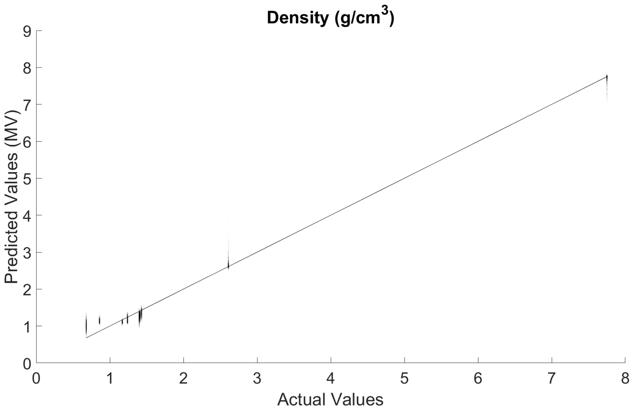
Figure 6 shows the comparison between the actual density values and those predicted by the multi-channel network using the combined approach. This is the combination of all results predicted for the testing data sets in all 90 of the different partitions. Given that this consists of 9000 points, the opacity of each of them was reduced to 3% to accurately depict their distributions. The combined approach improves on the R²-value from 98.417% to 99.107%.

4.3. Volume Estimation

The introduction of depth camera technologies (such as a Microsoft Kinect camera that uses a depth sensor based on a structured infrared-light system) opened new possibilities for estimating the volume of unknown objects. Several approaches are proposed to estimate the volume of an object in unknown environment, including the volume–intersection methods [25,26], height selection and height selection and Red-Green-Blue (RGB) segmentation [27]. Measuring the volume of unknown objects is beyond the scope of this research.

In this study, measuring the volume of the 10 samples involved measuring the dimensionality of rectangular samples, cutting the non-rectangular samples into rectangular shape (normalization) or using measuring tubes to determine their volumes based on the change in water level in the tube before and after they are fully submerged. In the future, we plan to implement one of the off-the-shelf techniques for measuring the volume of these samples using an RGB-D camera (such as the work presented in [28]). An RGB-D camera produces images that contain a combination of color information (RGB) and depth information about every pixel in the corresponding RGB image. Depth information may help improve object identification and shape extraction.

5. Discussion

It is clearly visible that our result is very close to the 100%R²-value, which represents a perfect agreement between predicted and actual density values. However, it is worth putting this into perspective in order to gather insight about whether it is our approach that resulted in this high value, or the quality of our data, or whether it is a generally easy task to predict density from radiometric frames. This is where the results corresponding to the “baseline 1” and “baseline 2” models are particularly helpful.

The “baseline 2” model, being the simplest of the three variants, produced an R²-value of just over 50%. This is the proportion of variance in the target data set that is “explained” by the model as opposed to simply predicting the average of the data set for each value, which would yield an R²-score of 0%. This means that there is some fairly basic information in the radiometric frames that even this simple model can find. However, switching to a neural network such as the “baseline 1” network results in a significant improvement, at the cost of a roughly 4× increase in the number of parameters. This shows that the benefits of a convolutional neural network are apparent even when the network is very shallow (compared to parameter numbers in the 10⁷-range for some state-of-the-art Convolutional Neural Networks (CNN) [29]).

Though the results of the “baseline 1” network are encouraging, our multi-channel approach manages to outperform it. The 0.75% difference in the respective R²-values is not huge, but, given how close both these values are to a prefect prediction of 100%R², the improvement had a very small upper bound in the first place. It is therefore worth looking at this comparison in terms of the proportion of variance that is not explained by the networks. This value is 2.326% for the “baseline 1” model, and 1.583% for the multi-channel approach. This is a 32% relative error reduction, which demonstrates the real magnitude of the effect of adding the time stamp input to the network. Moreover, it has to be emphasized that switching from "baseline 1" to the multi-channel network adds less than 0.3% to the complexity of the network.

The fact that these results were achieved using an extension of a relatively simple and shallow convolutional network is promising for two reasons. Firstly, further reductions in the error term are likely to be achieved using sufficiently more complex extensions of this multi-channel framework. Secondly, a more complex network is also bound to be more robust to being trained on a higher amount of samples.

The most interesting observation about these results is that the system managed to find an effective connection between different types of material properties, over a large scale. The radiometric images acquired by the thermography setup show differences in how heat spreads on the surface of a material. This is largely an effect of different thermal conductivity and thermal diffusivity values over these materials. The system has managed to translate these differences into predicting a different material property, the density values of the samples. This can be done by either finding a direct (likely nonlinear) relationship between these properties, or by taking an indirect approach and classifying the materials based on their thermal properties, then assigning the target density value based on existing knowledge acquired during the training procedure. In the specific case of this study, the results seem to contain elements of both approaches, as the system is capable of distinguishing marble and steel from the rest of the samples, for example. However, the continuous spectra of predicted values assigned for each sample demonstrate a genuine regression-focused approach for the network.

It is worth mentioning that the proposed methods are insensitive to sample shape. During the measurement, only a small amount of the surface of the object (<1 mm²) is subjected to excitation. Moreover, due to the short amount of time between the beginning and the end of the measurement, this excitation results in non-negligible heating in only a limited area around the center of excitation. As long as this surface area of the material (<1 mm²) is sufficiently flat and the material is thicker than a few millimeters at the excitation center, the system should work fine.

Although the results from the realization of the weight estimation framework are promising, a number of limitations should be noted. First of all, the sample set is a small one. Even though great effort is put into forming the set in order to cover a variety of materials and material properties, future work must consider increasing the number of samples significantly. Another limitation is that the realization of the proposed framework did not take into consideration the effects of emissivity and surface texture. In more practical scenarios, these assumptions are not necessarily valid and thus the effects of emissivity and surface texture on density (and thus weight) estimation must be studied. Machine vision (using RGB camera) may be used to extract these properties using computer vision technologies and use them as auxiliary inputs to the neural network to compensate and improve weight estimation. Furthermore, due to the use of visible lasers that might be harmful to humans, the application of the proposed system for estimating the density of human tissues could not be practical. Finally, the proposed approach relies on computer vision to estimate the volume of the object. However, the proposed approach may not work properly with hollow objects for objects with inhomogeneous materials (such as a cup with water). In such cases, machine vision may compliment the proposed approach to improve the estimation accuracy/applicability.

6. Conclusions and Future Work

In this article, we proposed a framework for estimating the weight of unknown objects by estimating their density and volume through separate processes. With volume estimation having been demonstrated effectively in the past by others, we have presented a system that uses infrared thermography and a custom multi-channel neural network to perform density estimation. The results demonstrate the validity of our approach and its superiority compared to other machine learning implementations without any meaningful increase in complexity. Topics left to investigate in the future include testing the network and its variants on an expanded sample size, integrating the entire system onto a single-board computer to enable mobile applications such as in robotics, and examining if any other physical properties can be estimated or inferred through the combination of infrared thermography and machine learning.