Tactile-Driven Grasp Stability and Slip Prediction

Abstract

One of the challenges in robotic grasping tasks is the problem of detecting whether a grip is stable or not. The lack of stability during a manipulation operation usually causes the slippage of the grasped object due to poor contact forces. Frequently, an unstable grip can be caused by an inadequate pose of the robotic hand or by insufficient contact pressure, or both. The use of tactile data is essential to check such conditions and, therefore, predict the stability of a grasp. In this work, we present and compare different methodologies based on deep learning in order to represent and process tactile data for both stability and slip prediction.

1. Introduction

Tactile sensors provide a rich source of information regarding the contact a robotic hand or gripper experiences during a grasp or the manipulation of an object. As Kappassov et al. [1] showed in their review, these sensors have been used for estimating physical properties of objects or even detecting in-hand events like slippage. In this fashion, Luo et al. [2] reviewed multiple ways a tactile sensor can record pressure or force signals and how they can be processed in order to perceive properties like material stiffness, shape or pose, among others. Some examples of these applications are the works of Kerzel et al. [3] and Liu et al. [4], who approached the task of recognising a material by performing touches throughout its surface, as well as the works of Schmitz et al. [5] and Velasco et al. [6], who approached the recognition of grasped objects with multi-fingered hands.

Another interesting application is the control of robotic hands or grippers in order to keep stable grasps. In those cases, tactile sensing drives the slippage detection of an in-hand object so the robotic system can correct it by changing the hand pose or the pressure applied. In this line, van Hoof et al. [7] used reinforcement learning and tactile feedback in order to learn to perform a rolling action of an object. Hang et al. [8] proposed a whole system which generated potential grasps, executed optimal grasps and also performed an in-hand grasp adaptation, combining visual, tactile and proprioceptive feedback. Recently, Calandra et al. [9] used an optical-based tactile sensor in order to train a robot so it could use tactile information for adjusting grasps as well, simultaneously processing raw visuo-tactile data and effector poses during the grasp.

In order to build a tactile-driven controller, a stability and slip predictor is needed for giving a feedback regarding the state of the grip. In this work, we exploit this type of data for approaching the prediction of the stability of a grasp and the detection of the direction of slip of a contacted object. Since we use a non-matrix tactile sensor, our goal is two fold: first, we propose two ways of interpreting non-structured tactile data in order to learn deep features; and second, we report the performance yielded by deep learning techniques on these two tasks using two custom datasets.

1.1. Types of Tactile Sensors

In the last years, a variety of technologies are being used in order to manufacture tactile sensors: piezo-resistive, capacitive, optical, ultrasonic, based on piezo-electric materials, based on magnetic transduction and based on barometric sensor, among others. Recently, Yi et al. [10] presented a review of some of these tactile transduction techniques. The most known for robotic hands and grippers are commented below:

• In a piezo-resistive sensor [11], the resistance of the materials changes when a force is applied. The advantages of this sensor are its wide dynamic range in the measurements, the low cost of manufacturing it, its simple integration and its great durability, although it has low spatial resolution and can produce hysteresis.
• Capacitive sensor [12], in which the distance between two plates changes when a force is applied. Its advantages are good integration, high sensitivity, stability and its ability to sense normal and tangential forces. However, it can produce hysteresis too.
• Optical sensor, which uses a camera to measure the visual deformation of a pattern in an internal surface. The main advantage of this type of sensors is that it is immune to electromagnetic interferences, it has a quick response and high spatial resolution. The disadvantage is that it is usually large. One of the most known is the GelSight [13,14].
• Based on magnetic transduction [15]. This sensor measures changes in the flow density of a small magnet caused by the applied force. It stands for its high sensitivity, also for providing a good dynamic range and it can detect multi-direction deflections. Its response is linear and without hysteresis. Moreover, its manufacturing materials are robust.
• Barometric sensors, which measure the pressure of a contact from the deformation of a liquid or air contained inside the sensor, affecting the electric current registered by a set of electrodes. An example is the BioTac sensor [16] used in this work.

1.2. Tactile Data Processing

Due to the base technology of a sensor, tactile readings can be represented either as a continuous signal, a set of discrete measurements on tactile cells or as a sequence of images. For example, a piezo-resistive sensor would output a single signal with the change in its resistance when a force is applied. In a barometric sensor like the one we use in this work, the output would be more than one of those signals, which could be arranged in vectors. Capacitive sensors usually provide matrices with values from a set of cells into which the sensor is divided. Finally, optical sensors provide images, since their sensing system is based on a camera. The structure of the tactile data a sensor provides could influence the set of techniques or algorithms that can be applied in order to process them and learn from them. However, there are ways to interpret these data in other structures.

If the tactile sensor provides a global pressure value, then the best representation could be a signal that shows the variation of that value through time. However, if the sensor consists in a set of electrodes or sensing cells which provide a pressure value for each of them, then a more powerful representation is a tactile image: a matrix in which each pixel represents a pressure reading instead of a colour value. A sequence of images, therefore, could represent a set of tactile readings acquired at different moments. Using tactile images, instead of using signals from each cell or electrode separately, exploits a unique normalised format that keeps spatial information among sensing points located in a same neighbourhood area. In this trend, Delgado et al. [17] and Zapata-Impata et al. [18], defined two different ways of representing tactile readings in an tactile image for sensors whose output is not naturally arranged in matrix-like distribution – like in the case of cameras or capacitive sensors–, showing results that seem to prove that tactile images are of great value for learning to detect useful patterns in manipulation tasks. Lately, Garcia-Garcia et al. [19] have presented a novel way to interpret tactile values from those unstructured sensors using graphs, establishing an alternative to tactile images.

It is possible to learn from tactile readings using traditional machine learning techniques in order to approach problems in robotic manipulation and grasping. For such purpose, one can extract tactile features or descriptors. In the past, Kaboli et al. [20] built tactile features from raw tactile signals and then used them for training a Support Vector Machine (SVM). This was later extended by designing a transfer algorithm based on Least Squared-SVM, so texture models could be built and later applied to object recognition [21]. In this line, Luo et al. [22] presented a modified SIFT descriptor for tactile data, which required that the raw readings were organised within a matrix like an image. Similarly, Yang et al. [23] used sequences of tactile images and covariance descriptors to capture object properties, such as texture and roughness.

However, it is also possible to directly input raw tactile readings into a machine learning model and learn the features in the process. For example, Spiers et al. [24] extracted some manually features which were mixed along with the raw tactile readings in the input of a Random Forest (RF) for the task of object classification. More recently, deep learning techniques are being used to achieve this automatic learning of features, without considering the kind of sensor used to obtain the tactile information. Gao et al. [25] explored the possibility of learning tactile features using both Convolutional Neural Networks (CNNs) and Long Short-Term Memory (LSTM) networks for the task of recognising object properties. In this line, Li et al. [26] experimented with multi-modal data for slip detection: the authors combined visual features and tactile features learnt from a camera and a GelSight sensor using CNNs, which were introduced into an LSTM throughout a grasp action. More recently, Zhang et al. [27] and Zapata-Impata et al. [28] used Convolutional LSTM (ConvLSTM) networks in order to learn spatio-temporal tactile features, which encoded both the changes in the local connectivity of the sensing points as well as their individual change through time.

Nowadays, the area of tactile perception could be compared to the field of computer vision: we come from an era in which tactile data was processed in order to generate descriptors which were hand-engineered, but the current trend is showing that deep learning techniques can achieve competitive results without the need of designing those features, though requiring datasets, computing power, training time, among others. In this work, we approach the tasks of grasp stability prediction and direction of slip detection from this learning perspective, so we use raw tactile values as an input for our deep learning models. Moreover, despite it has been proved in the literature that mixing multi-modal data like vision, touch, sound and/or proprioception improves the performance of a robotic system [4,29,30,31], we only use tactile perception. Although this could be seen as a limitation, our objective is to evaluate the performance of these deep learning models using only the registered responses from our unstructured tactile sensors.

2. Related Works

Grasp stability estimation with a robotic hand or gripper is a challenging task in environments with uncertainty as when the grasped object is unknown. This is more complex when the object is soft or deformable and therefore it is difficult to obtain contact measures by applying force closure grasps. The same complexity applies to the detection of slippage, and it is increased in the case of the classification of such slip event in various translational and rotational directions.

Regarding the prediction of stability, Bekiroglu et al. [29] proposed two approaches: one based on a single tactile reading at the end of the grasping action, in which they used SVM and AdaBoost; and another based on temporal tactile series obtained throughout the grasp, in which they used probabilistic learning based on Hidden Markov Models (HMM). Similarly, Schill et al. [32] also employed HMM but combined with the output of a SVM, which used moments extracted from the tactile readings. Cockbum et al. [33] used an unsupervised feature-learning approach to find the common denominator behind successful and failed grasps in order to predict whether a grasp attempt would be successful or not. They used an auto-encoding strategy by combining a dictionary, a reconstruction phase, training and classification with SVM. Later, the same authors extended their work adding proprioceptive data and shifted to a supervised strategy based on CNN [34]. These works showed significant results in this area, but they combined proprioceptive data along with their tactile information. Moreover, their tactile sensors provided a stream of responses structured in a matrix so they could work directly with them as if they were tactile images.

Regarding the detection and classification of slip events, Reinecke et al. [35] and Veiga et al. [36] discussed slip detection strategies using the BioTac sensors. Since these sensors are not arranged in matrix-like distributions, the authors calculated features that were later learned by a RF or a SVM in order to predict slippage. In contrast, Su et al. [37] concatenated consecutive raw readings from a BioTac sensor and fed them directly to a shallow neural network in order to detect slippage. These works showed that BioTac signals could be precise enough to approach this task and that they might hold relevant patterns for it. However, they only worked on the problem of detecting a general event of slippage and, some of them, needed hand-engineered features to achieve such goal.

Heyneman and Cutkosky [38] experimented with various types of tactile sensors in order to approach a more complex slip detection: their system could detect slippage between the tactile sensor and the object held, or between the object held and the environment. Despite showing relevant results with high accuracy rates in this task, the tactile signals had to undergo a preprocessing step in order to calculate features. In contrast, Meier et al. [39] explored the possibilities of CNNs for the task of slip and rotation detection. Consequently, the authors did not have to design features because they were learnt by the CNN instead. The authors distinguished between a rotational and a translational slip in their task, increasing the complexity of the detection task. However, their system used large tactile matrices (16 × 16 cells, measuring each cell 5 × 5 mm) which could not be installed in a robotic hand. In this line, Dong et al. [40] also considered translational and rotational slip. The authors showed various methods for tracking slippage which did not require the computation of features nor training neural networks, though they could only be applied to the tactile images generated by the GelSight since they were based on the markers contained in those images. Similarly, Zhang et al. [27] used a optical-based tactile sensor in order to distinguish a slippery grasp from a stable one. However, they realised that slips are spatio-temporal events so they experimented with a ConvLSTM, achieving state-of-the-art results on this task. Nevertheless, their system only detected two grip states: stable or slip.

Unlike other researchers, we explore different ways to interpret tactile data from a sensor which is neither structured as a matrix nor contains a camera. We explore this in order to approach two robotic tasks: stability prediction and slip detection. In contrast to previous works, we do not aim to design tactile features but our focus is on preparing the tactile data so a deep learning model can learn them. Moreover, we work on a more complex task in the case of slip detection: current proposals in the literature just classify two types of slippage at most (translational/rotational) but we work on six directions for the slip events. Besides, we evaluate the impact of tactile data on these tasks without using additional information as vision or proprioceptive data. The two problems approaches, the sensor used and its processing are described along with the learning techniques in Section 3. Then, achieved results are presented and discussed in Section 4. Finally, we give our conclusions in Section 5.

3. Materials and Methods

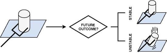
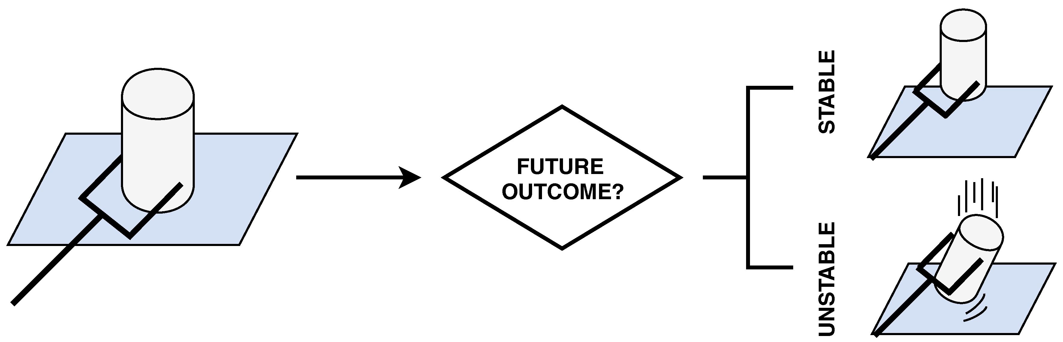
3.1. Problem Statement

In this work, we approach two robotic problems. One is the prediction of the stability of a grasp. More precisely, we want to predict the future outcome of a robotic grasp, labelled as stable grasp or unstable grasp, using as the main source of information a single snapshot of the state of a set of tactile sensors (see Figure 1). That is, a system must learn from a set of static tactile readings acquired at a single moment in time, which are obtained when the robotic gripper has contacted the object but it has not lifted it yet. Therefore, the system must predict that the grasp is stable if the object is lifted without falling or slipping. This problem is important for preventing failures since there are scenarios in which an unstable grasp can result in broken items.

The other problem here covered is the detection of slip direction. While a robot carries an object within its gripper, the object can suffer perturbations that lead to motions of the object in hand. As a result, the grip might become unstable and, consequently, the object might slip from the robotic hand. The task of direction of slip detection aims to detect the type of slip that is occurring while the robots still keeps the grip on the object. Two main groups of events are distinguished here: translational slip, with four main directions (north, east, west, south); rotational slip, with two main directions (clockwise, anti-clockwise); and also the lack of slip (stable). See Figure 2 to find an example of each of these main directions of slip.

Tactile data can be used to approach this problem as well. In contrast to the stability prediction, the detection of slip direction has a temporal component: slips occur through time and therefore, tactile data varies through time while the sensor experiences a type of slippage. Hence, a detection system for this task must learn from a temporal sequence of tactile readings, since a single snapshot might not provide the system with sufficient information for distinguishing the direction of the slip.

3.2. Tactile Sensor

BioTac (BioTac^® from SynTouch Inc., Montrose, CA, USA) is a biomimetic tactile sensor inspired in the human sense of touch and its size is similar to the human fingertip [41]. All of the sensing points in the BioTac device lay within a rigid core surrounded by a elastomeric skin that is filled with a conductive liquid. The electrical resistance of the conductive liquid trapped inside between the elastomeric skin and a set of electrodes and emitters on the sensor’s core is used to measure the distribution of forces applied on the surface. In addition, the fingertip surface imitates a fingerprint to produce friction and vibrations by contact when the fingertip is sliding on another surface. When the BioTac sensor is used to explore the surface of an object, it is able to detect the position of contact point, both normal and tangential contact forces and it can also measure some variations of temperature via a set of heaters in conjunction with a thermistor.

In our work, we use the BioTac SP, which is an improved version of the BioTac. It differs in its geometry, the number of electrodes and in the sampling frequency used to obtain data. BioTac SP was designed with an elliptical shape, therefore the distribution of electrodes on the fingertip surface is different to BioTac as observed in Figure 3 (left). BioTac SP has 24 electrodes distributed throughout its internal core vs 19 of the former BioTac.

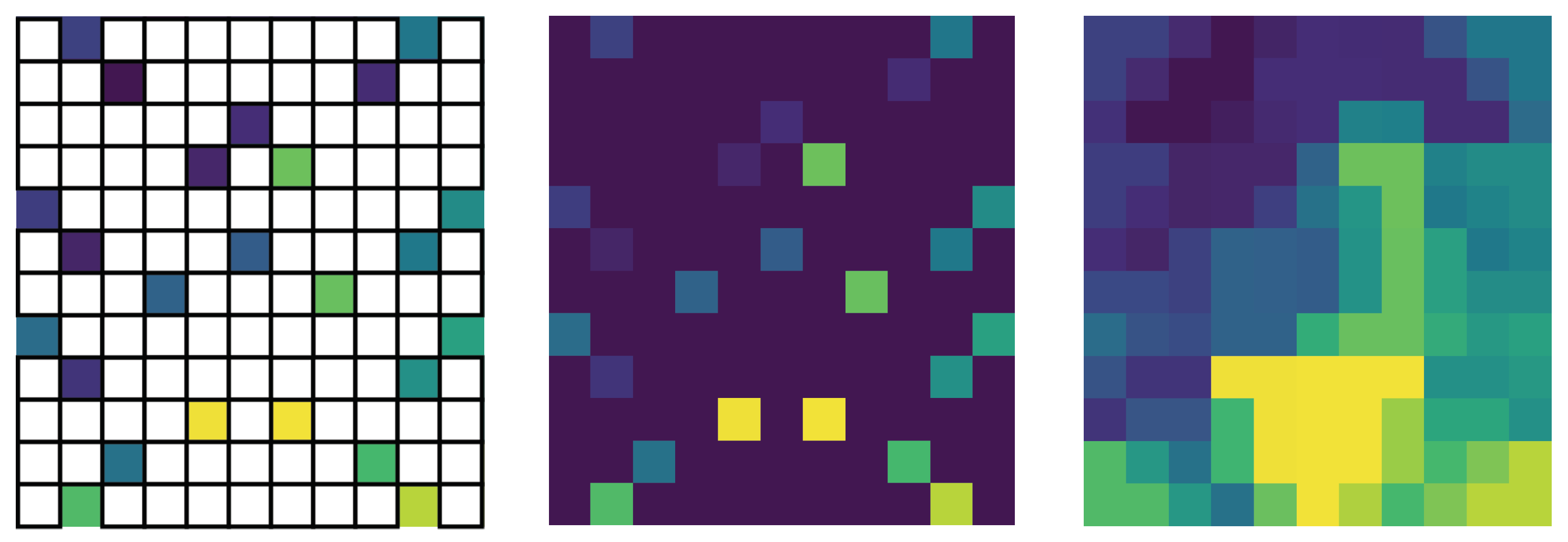
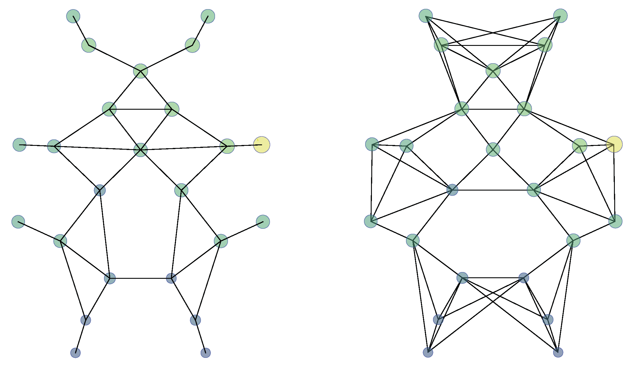
3.3. Data Interpretation

The pressure data obtained from the BioTac SP can be organised for its processing as tactile images (Figure 3 (right)). A tactile image $\varphi$ is a matrix representation of the data obtained from the 24 electrodes. However, the fingertip shape in the BioTac SP is not a flat surface so the electrodes are distributed in a 3D space. In order to create tactile images from a non-matrix tactile device, we propose to design a matrix in which pixels are filled with the electrodes data, but looking for a distribution similar to the projection of 3D coordinates $p_i=(x_i,y_i,z_i)$ on a plane with 2D coordinates $(u_i,v_i)$, being $i=\{1,\dots ,24\}$ and $(u_i,v_i)$ the pixel coordinates of the tactile image I. Thus, we can keep the local connectivity among any electrode and its neighbouring with this type of representation. Afterwards, we assign an intensity value for each pixel depending on the pressure value of its corresponding electrode.

Depending on the size chosen for the tactile image $\varphi$, the projection of the 3D coordinates of the electrodes to the pixel coordinates provide us a distribution more or less compact, as shown in Figure 3. When we build the tactile image, there are pixels that do not correspond to any electrode and therefore we cannot assign a value from the pressure measured. The reason for this is that there are already areas in the surface of the sensor without electrodes. In these cases, we have to fill these gaps so that the pixels have a value. There are some simple strategies to fill these missing values: fill these missing values with the value of the less contacted electrode or fill them using the mean of their k neighbours (see Figure 4). In this way, we built a tactile image ${\varphi }_j$ from electrode readings for each of the three fingers used in the robotic manipulation task, being ${\varphi }_1$ the index, ${\varphi }_2$ the middle, and ${\varphi }_3$ the thumb.

Another approach for preserving the connectivity of the sensing points is to use a graph as a structure for representing the state of the sensor in a given moment. One of these graphs can be defined as a triplet $G=(N,E,Y)$, where N is a set of 24 nodes $N=\{n_1,n_2,\dots ,n_{24}\}$ (one node per electrode), E is a set of edges or connections between nodes and Y is the category or label of the graph for a classification task.

Each of the nodes in the graph $n\in N$ are characterised by a 3D position $p_n=(x_n,y_n,z_n)$ and a feature vector $f_n=(f_{n1},f_{n2},\dots ,f_{nm})$ of length m. Positions $p_n$ were mapped from the 3D coordinates of each of the 24 electrodes, which were provided by the manufacturer. These coordinates are defined with respect to the centre of the sensor’s internal core. As for the feature vector, since we count with three BioTac SP tactile sensors, we decided to define these features with the pressure readings of the three fingers. That is, a given node n has three features $f_n=(f_{n1},f_{n2},f_{n3})$, where $f_{n1}$ is the pressure reading from the n-th node (electrode) from the sensor installed on the index, $f_{n2}$ is the reading from the middle sensor and $f_{n3}$ is the reading from the thumb.

Regarding the set of connections or edges E, they can be generated with two strategies: we could manually specify which nodes are connected following some particular criterion like symmetry; or they could be generated using a vicinity method, such as k-Nearest Neighbours (k-NN)? These connections can be directed, meaning that an edge $\{n_i,n_j\}$ connects the node $n_i$ with the node $n_j$, but not in the other way. However, graphs can also be undirected, so an edge $\{n_i,n_j\}$ connects both the node $n_i$ with the $n_j$ and the $n_j$ with the $n_i$. In our work, we manually defined undirected connections for defining a graph, but we also tested directed graphs using the k-NN strategy. See in Figure 5 an example of a graph with manually generated, undirected edges and another graph with directed connections generated with $k=4$.

3.4. Learning Methods

In this section, we describe the techniques used in experimentation with the BioTac sensor, which we divided in two main groups depending on the approached problem and the selected data structured used to process tactile values: deep neural networks fed with static tactile values (obtained at a moment in time) and deep neural networks trained with temporal sequences (obtained at a time interval) in order to address problems like stability prediction and direction of slip detection.

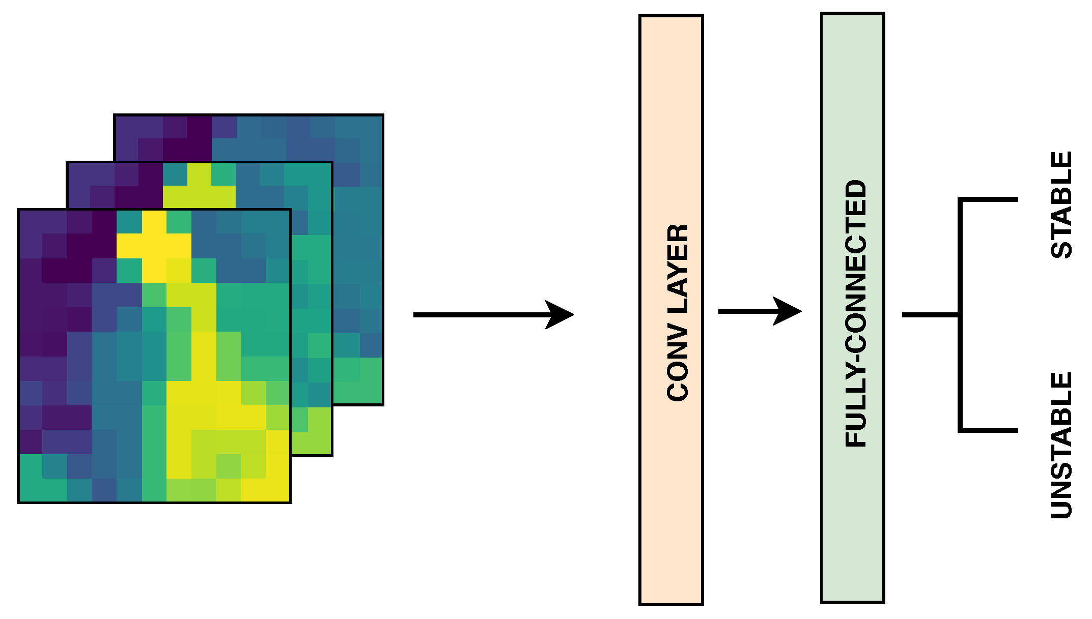
3.4.1. Deep Neural Networks for Static Data

In the case of problems like slip detection, tactile readings recorded from a single contact of the gripper with the object are frequently used. This type of static data can be processed in various ways, though recent trends suggest the use of Convolutional Neural Networks (CNN) [42] since most of the latest works on this field are using optical tactile sensors [43]. These type of networks have proven to outperform other methods in image classification tasks, owing to its ability to learn image features by itself [44].

Basically, a CNN receives as an input an image I that is composed of pixels in a 2D space and might have multiple channels (i.e., RGB). The convolutional layers process the image I with multiple kernels or filters, resulting in another image $I^{\prime }$ with new dimensions, which continues through the rest of the layers of the network. There can be pooling layers for reducing the dimensions of the intermediate images $I^{\prime }$. At the end, a set of fully-connected layers perform the last steps of the learning before giving as a result a probability of the input image to belong to a set of target categories.

In the case of using an optical tactile sensor, the processing carried out by a CNN is not different, since the readings from this type of sensor are actual pictures. However, if one uses a tactile sensor like the BioTac SP, a pre-processing step is necessary for transforming the readings $\theta =\{e_1,e_2,\dots ,e_{24}\}$ into a tactile image $\varphi$. Once that step is completed, the CNN can learn to detect stability patterns from the tactile readings. Figure 6 shows an example of a CNN that receives as input a 12 × 11 × 3 image I, which holds three tactile images $I=\{{\varphi }_1,{\varphi }_2,{\varphi }_3\}$ of size 12 × 11, one for each finger used in the manipulation task. This image could be generated from a snapshot at the same time of three tactile sensors installed on a multi-fingered robotic hand.

In our experiments, we trained a CNN with 32 convolutional 3 × 3 filters followed by Rectified Linear Units (ReLU) and then a fully-connected layer with 1024 ReLU units. Finally, this layer was connected to a softmax layer in order perform the classification of grasps. Other configurations were tested, including pooling layers, as well as more convolutional layers with bigger filters. However, increasing the size of the filters and pooling the intermediate results showed to be detrimental because these techniques reduced too much our input, losing useful information for the learning model.

As described previously in this document, another way to interpret tactile readings from the BioTac SP sensors is as tactile graphs. Lately, Graph Neural Networks (GNNs) have emerged as an alternative way to learn from data that can be structured as a graph. Kipf and Welling [45] proposed a straightforward generalisation of convolutions to graphs, defining the CNN-like network for processing graphs: the Graph Convolutional Network (GCN).

A GCN takes as input a feature matrix X with size $NxF$—there is a feature vector $f_n$ for each node n in the graph G—and an adjacency matrix A that shapes the graph. As with the convolutional layers in a CNN, the graph-convolutional layers in a GCN process this input in order to learn nodel-level features, making using of the adjacency matrix A in order to check the neighbours of each node during the convolutions, and then output another feature matrix $X^{\prime }$ with size $Nx{F}^{\prime }$—there is a new feature vector $f_n^{\prime }$ for each node n. Again, there can be pooling layers for reducing the size of the intermediate graphs. At the end, fully-connected layers are appended to the network and a probability of the input graph to belong to a set of target categories is returned. Figure 7 shows a GCN that receives as input a graph G in which every node n has a feature vector $f_n=(f_{n1},f_{n2},f_{n3})$—the three features are decoupled in three graphs in the figure for visualisation purposes. This graph could be generated from a snapshot at the same time of three tactile sensors, so every feature $f_{ni}$ is the value of the n-th electrode $e_n$ from the reading $\theta$ acquired using the i-th tactile sensor.

In our experiments, we tested GCN configurations with different number of layers and units. Given the size of our input tactile graphs (24 nodes with 3 features) the best configuration found had five layers with $8,8,16,16$ and 32 units, respectively. At the end, two fully-connected layers with 128 and 2 units received the processed graphs in order to finally perform the classification. Initial experiments showed that increasing further the complexity of the network did not improve the performance of the model in our task. Regarding the connectivity of the graphs, we tested manually generated connections, as well as a strategy based on k-NN, as shown in Figure 5. It was found that using less connections improved the performance, being our manually generated graph the best option.

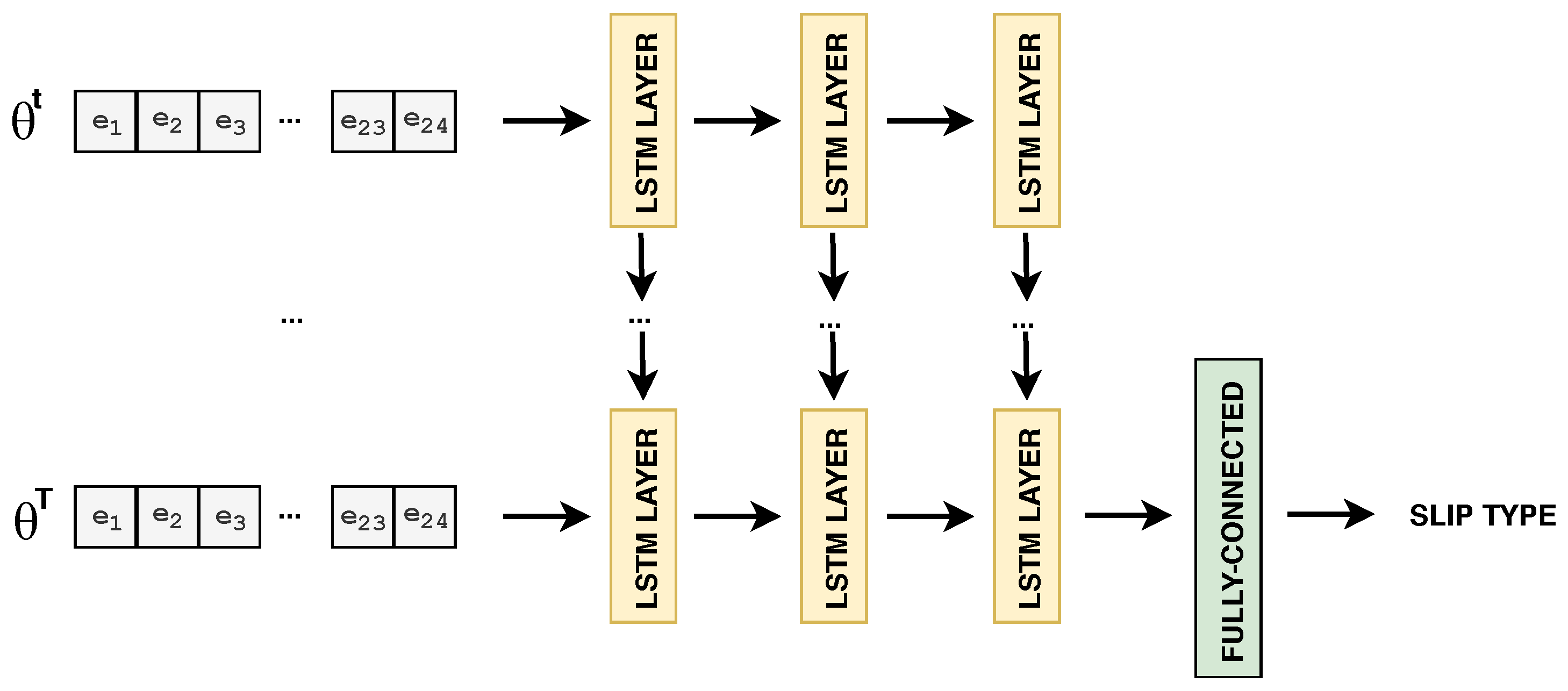
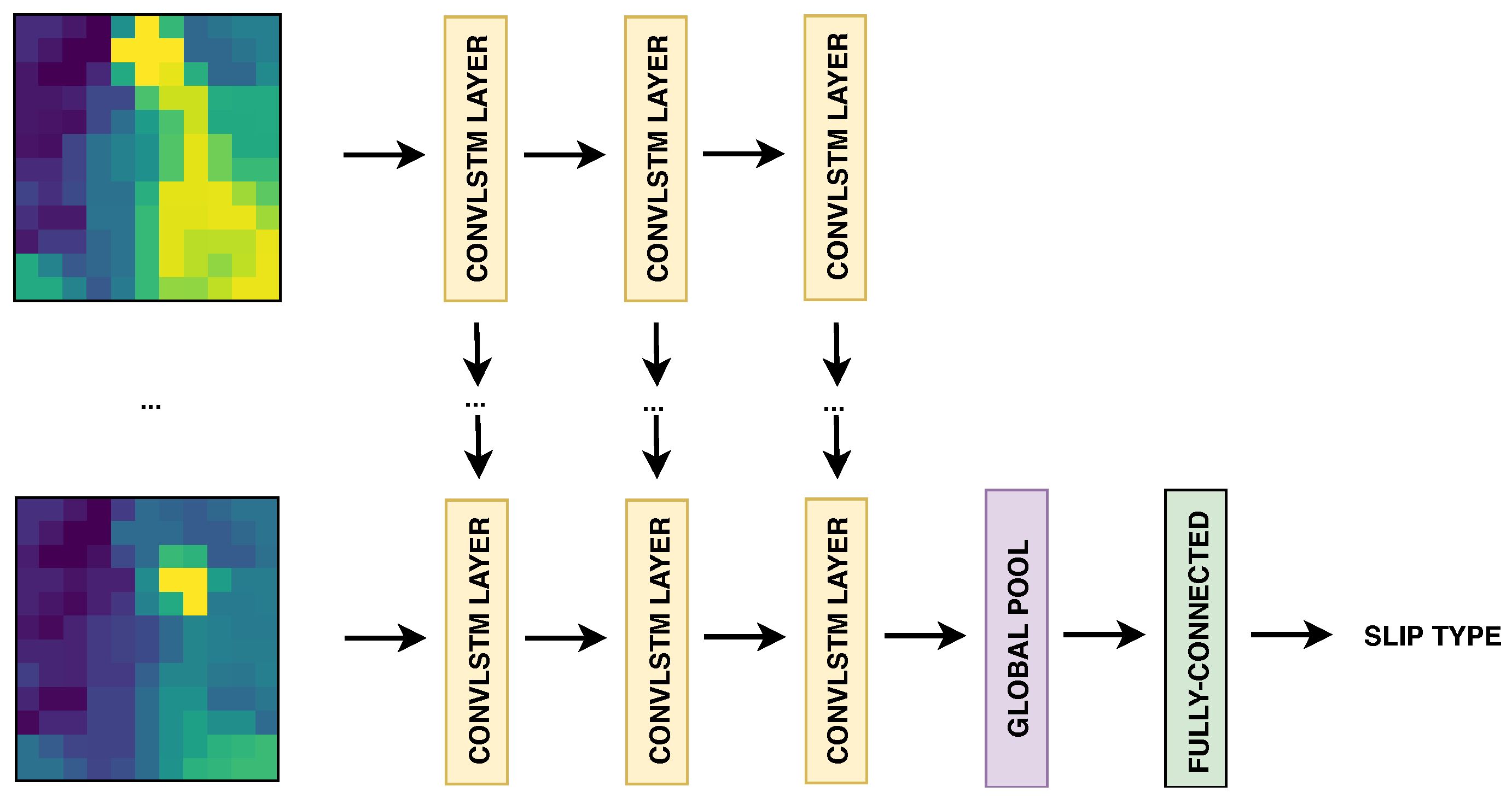
3.4.2. Deep Neural Networks for Temporal Sequences

Problems like the detection of slip direction require gathering sequences of tactile data in order to check the variation of the readings through time. In order to learn from such type of information, methods presented in the previous section are limited for one main reason: although they could concatenate temporal sequences in channels (for a CNN) or more features (for a GCN), there would not be such concept of order nor memory. For that purpose, we make use of another type of networks.

On the one hand, we used an architecture based on Long Short-Term Memory (LSTM) networks [46]. These networks have a special type of unit in its layers that not only take as input the data used for training but also its own output. That means that the output of a layer $H_i$ is connected to both the following layer $H_{i+1}$ and the layer itself $H_i$. Therefore, the network behaves in a temporal way which is appropriate for learning from temporal sequences. During the processing of an input sequence $X=\{x_t,x_{t+1},\dots ,x_{t+m}\}$, the LSTM unit takes the $x_i$ values one by one at each moment t and keeps a state stored in a memory cell $c_t$. Through the use of some operators, the unit decides whether it should accumulate the new input $x_{t+1}$ in the memory, forget the previous state that comes from $c_{t-1}$ and also if it should operate its current value $c_t$ with the layer’s output. As well as the CNNs and GCNs, the LSTM networks also include fully-connected layers at the end before giving the output of the classification.

Through the use of this type of networks, it is possible to learn to detect the direction of slip using raw tactile readings. That is, if one reads a sequence of T tactile readings $\mathsf{\Theta }=\{{\theta }^1,{\theta }^2,\dots ,{\theta }^T\}$, holding every reading the values from the 24 electrodes in the BioTac SP sensor ${\theta }^t=\{e_1,e_2,\dots ,e_{24}\}$, it is possible to train an LSTM that takes as input the sequence $\mathsf{\Theta }$ and outputs the possible type of slip (north, east, west, south, clockwise, anti-clockwise, stable). Figure 8 shows an LSTM that takes this type of input. Note that the LSTM layers at a moment t receive as input $x_t$ the raw reading ${\theta }^t$ from one tactile sensor and then their output are passed to the following layer, as well as themselves. This is symbolised by the arrows pointing down towards the same layer in the next time step.

The process that LSTM networks carry out can be also executed using tactile images as input, $\varphi$. For doing so, instead of training a network with LSTM units, we have to use Convolutional LSTM (ConvLSTM) units [47]. The main difference with the LSTM are the type of operations performed inside of the network, but the logic keeps the same. That is, ConvLSTM networks still have a memory cell $c_t$ that keeps a state at moment t, and through the use of some gates it can determine what to do with it. However, ConvLSTM operates with 3D tensors instead of 1D vectors so it performs convolutions with the data that goes through it (Figure 9). Therefore, one can use tactile images from a temporal sequence for training a ConvLSTM and learn both spatial and temporal features. In this case, the temporal sequence T of tactile images $\varphi$ built from a BioTac sensor can be represented as $\mathsf{\Phi }=\{{\varphi }^1,{\varphi }^2,\dots ,{\varphi }^T\}$ where each ${\varphi }^k$ is a tactile image built from the 24 electrodes in a BioTac SP and filling the gaps with the technique previously described in Section 3.3.

In detail, the results showed in this document were obtained using a ConvLSTM with five ConvLSTM layers (32 filters of 3 × 3) followed by a global average pooling layer and two fully-connected layers with 32 units and ReLU activations. Initial experiments showed that increasing further the complexity of the network—adding more layers, units or augmenting the size of the filters—reduced the generalisation capabilities of the network because it overfitted to the training data. Regarding the LSTM used in experimentation, it had a similar configuration but used common LSTM units in its layers, instead of the ConvLSTM layers.

4. Results and Discussion

In this section, we analyse the performance of the learning models discussed in the previous section. They were used to predict stability and direction of slip detection as learning tasks in robotic manipulation (Figure 10). Firstly, CCN and GCN models are used for stability binary detection, i.e., stable grip and unstable grip. Secondly, LSTM and ConvLSTM models are built to classify the type of slippage in the following cases: lack of stability, translational (up, down, left, right), or rotational (clockwise, anti-clockwise).

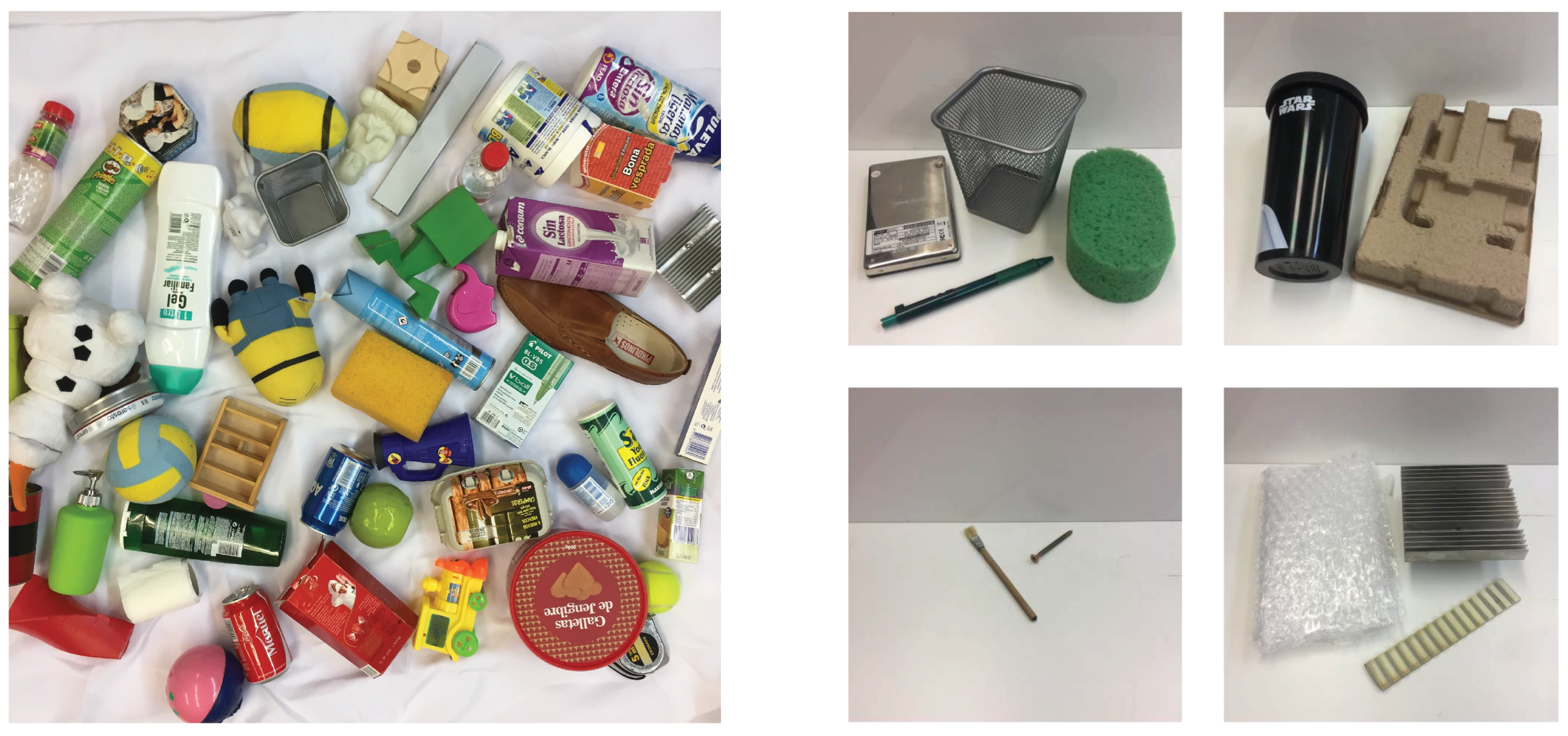
4.1. Dataset and Training Methodology

We generated two datasets in order to carry out the experiments: one for the stability task (see Figure 11 (left)) and another for the classification of slippage (see Figure 11 (right)). The first dataset is composed of 51 objects with three different geometries, such as cylinders, spheres, and boxes. Furthermore, we combined objects with different manufacturing materials, such as wood, plastic, and metal, as well as stiffness degrees. We recorded more than 5500 grasps, from which $80\%$ were used for training and $20\%$ for testing. Approximately $50\%$ of the data was recorded using the palm oriented in 45° with respect to the horizontal plane and the rest divided equally between the side orientation (90° with respect to the horizontal) and down orientation (totally parallel to the horizontal). These orientations were taken into account for recording the datasets because of the construction attributes of the BioTac: It has liquid inside which is affected by gravity so different orientations yield different tactile readings. In addition, the number of samples representing stable grasps and slippery grasps is similar so both subsets are balanced. More information, as well as the data, is available at [48]. Training and test sets were recorded following these steps:

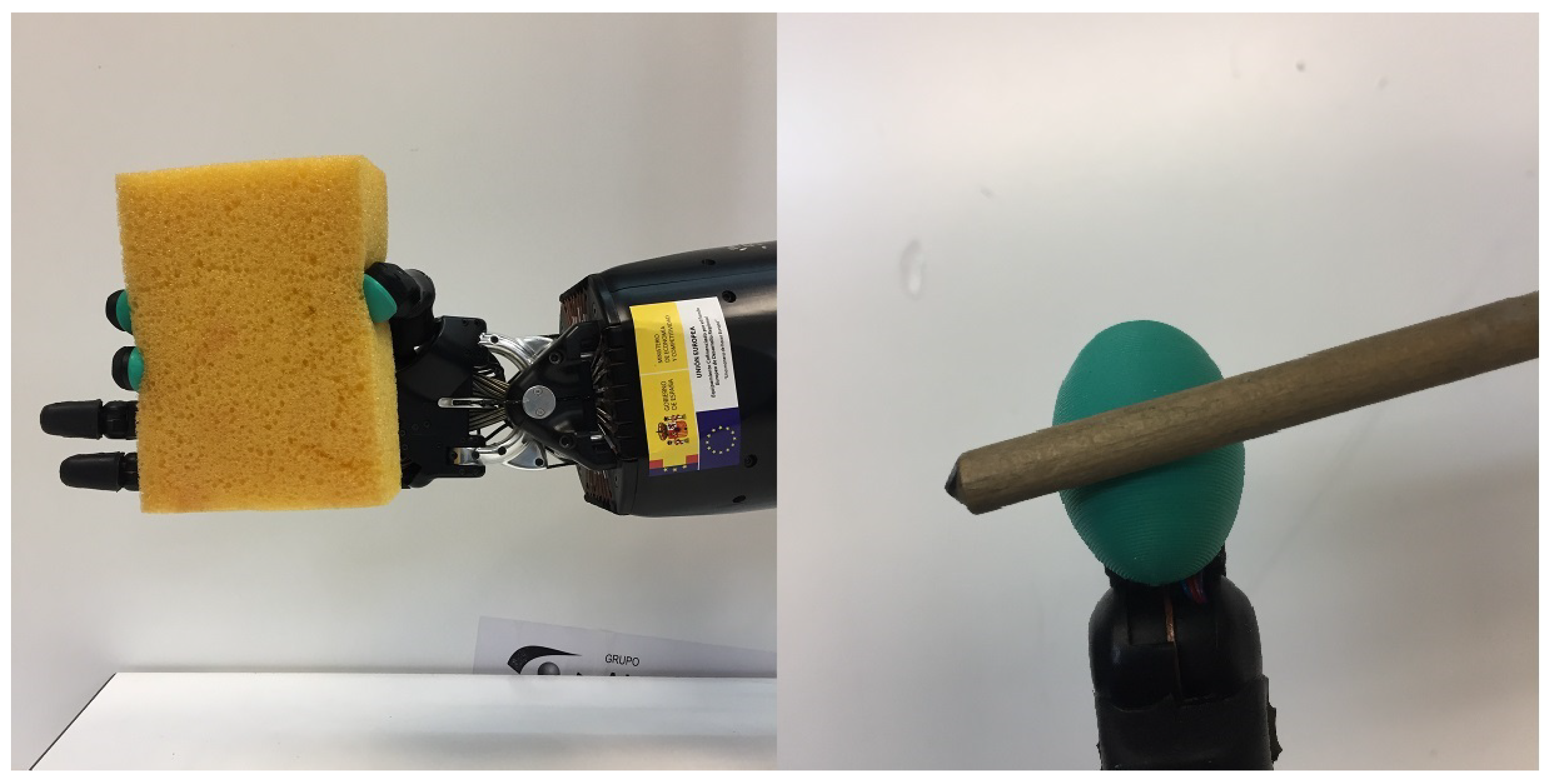
• Grasp the object: the hand performed a three-fingered grasp that contacted the object, which was laying on a table.
• Read the sensors: a single reading was recorded then from each of the sensors at the same time.
• Lift the object: the hand was raised in order to lift the object and check the outcome.
• Label the trial: the recorded tactile readings were labelled according to the outcome of the lifting with two classes; stable, i.e., it is completely static or slip, i.e., either fell from the hand or it moves within it.

Regarding the second task, we created a dataset with 11 different objects to those included in the previous dataset. We selected the objects by taking into account the stiffness of the material with which they were manufactured, the texture (i.e., rough or smooth surface) and the size of the contact surface—the fingertip is only in partial contact with the surface of small objects. The training was performed on four basic objects that hold various textures, sizes and stiffness degrees. In the testing step, we used seven novel objects which we grouped into three categories: two solid and smooth objects, two little objects with small contact surfaces and three objects with rough textures never seen before. In total, we recorded more than 300 sequences of touches, from which $36\%$ were used for training (the set of 4 basic objects) and the rest for testing, concretely $18\%$ for a first experiment with the two solid objects, $18\%$ for a second experiment with the two small objects and $27\%$ for the last experiment with the set of textured objects. The number of samples representing the seven directions of slip is similar so the set was balanced regarding the considered classes. More details, as well as the data, is available at [49]. In order to generate this dataset, we moved each of the objects over a BioTac sensor, producing a movement through each of the directions considered. The movement lasted for three seconds and it was carried out at different velocities and producing distinct forces. Moreover, each recording used a different part of the objects. Nevertheless, a single type of movement from each of the seven classes considered was performed on each sample. For the stable class, the object was pushed against the objects without motion.

Finally, training samples for both tasks were scaled to the range $[0,1]$ in order to ease the convergence of the neural networks. In addition, we used batch normalisation for improving the stability of the networks. Given that we are using deep learning models with datasets which are not large, the reported testing results were obtained from carrying out a testing stage similar to a 5-fold cross-validation in order to avoid overfitting to the training sets. That is, we found the best configurations using a typical 5-fold cross-validation with the training set. Then, we trained those configurations again shuffling the training samples and then launched predictions on the test samples. This last step of training and later testing was repeated five times in order to avoid reporting results achieved on a single pass through the train and testing phases. As a last remark, the sequences of tactile readings used for the direction of slip detection hold five consecutive readings in time. The publishing rate of the sensor is of 100 Hz; therefore, samples for this task have five tactile readings that were recorded in 50 ms.

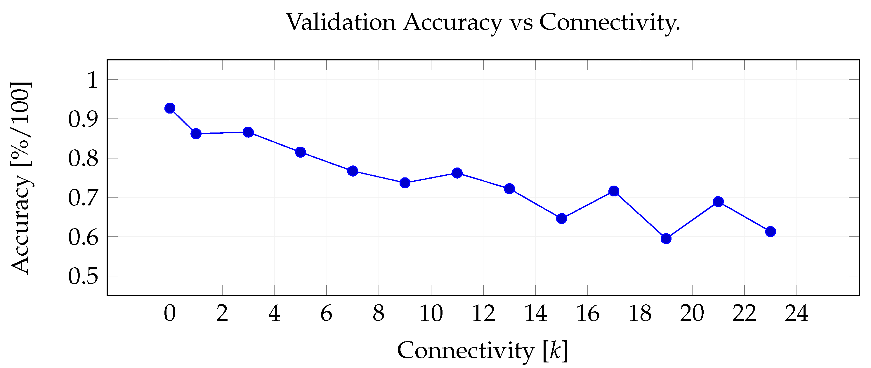
4.2. Tuning of Tactile Images and Tactile Graphs

First, we explored the effects of the three tactile distributions showed in Figure 3. To do so, we trained a basic CNN with a single layer of 32 convolutional 3 × 3 filters followed by a ReLU activation and then a fully-connected layer with 128 ReLUs. The training data were the recorded samples with the side and down orientations from the stability dataset. These samples were selected because we wanted to perform an exploration of the tactile distributions, so a smaller set was preferred. In total, 2549 samples were used for carrying a 5-fold cross-validation. Results are shown in

Table 1. Average performance in percentage (%) for each distribution tested.

Distribution	Accuracy	Precision	Recall	F1
D1 (12 × 11)	90.9 ± 1.5	90.4 ± 2.4	91.6 ± 2.4	91.0 ± 1.4
D2 (6 × 5)	89.6 ± 1.7	89.5 ± 2.8	89.9 ± 2.0	89.7 ± 1.5
D3 (4 × 7)	89.7 ± 1.3	89.7 ± 1.8	89.8 ± 2.6	89.7 ± 1.4

.

As can be seen, the three distributions achieve similar results on each of the four considered metrics. However, distribution D1 yields higher values on each of them consistently. This shows that distributing the sensing points from the BioTac sensor in such a way that they end up having similar neighbourhoods like in the actual sensor helps to obtain a greater performance. Moreover, D2 and D3 are close to the size of the kernel and there are less pixels to work with, forcing the learnt patterns to be less informative as well. Consequently, following reported results regarding the tactile images were achieved using D1.

Secondly, we also explored the effects of the connectivity graph in our tactile graphs. We showed in Figure 5 a manually generated graph but it was also mentioned the possibility of generating these connections using a k-NN strategy. This was tested on this experiment, showing Figure 12 the results obtained on the stability dataset by a GCN with five layers ($8,8,16,16$, and 32 units, respectively) and two fully-connected layers with 128 and 2 units. Let $k=0$ refer to our manual connections and $k=1,\dots ,23$ refer to graphs in which each node has connections to its k closest neighbours.

These results suggest that increasing the number of connections in the graph decreases the performance of the network. A bigger neighbourhood means that the convolution is basically taking into account more nodes in the graph. As a result, as the number of nodes in the convolution increases, the local tactile patterns in each area of the sensor are lost, because the convolution is basically using the whole sensor. This could be seen as a way of filtering out local information in favour of checking the general behaviour of the sensor. In contrast, in our manually generated graph, we connected some nodes to just another node, like those in the borders of the sensor, but some others are connected to various nodes in its neighbourhood, like the electrode in the centre. In consequence, there are different degrees of connectivity so there are various levels of importance given to local patterns. Therefore, reported results in following sections were achieved using the $k=0$ or manual distribution.

4.3. CNN vs. GCN: Image vs. Graph

We compared CCN and GCN models. Both models were used for stability binary detection, stable grip and unstable grip, from single touch data. Single touch data are tactile data obtained while grasping an object but prior to lift it. For this work, we recorded a total of 5581 tactile samples, distributed in 3 sub-sets depending on the orientation of the robotic hand (palm down 0${}^{\circ }$, vertical palm 90${}^{\circ }$, and inclined palm 45${}^{\circ }$). Our dataset contains tactile data of 51 objects with different properties, such as shape, material, and size. Each tactile sample was manually labelled according to two classes: 50% stable grip and 50% unstable grip. Later, the dataset was consequently divided into two mutually exclusive sub-sets: 41 objects were used for training and the remaining 10 objects were left for testing. This allowed us to check the generalisation capabilities of the proposed classification methods. Both models, GCN and CNN, were trained by exploring hyper-parameter tuning strategies, such as grid-search technique [50]. Thus, reported results were achieved with the best performing models found.

As can be seen in

Table 2. Detection results in percentage (%) on the test set for GCN (tactile graph) and Convolutional Neural Network (CNN) (tactile image).

	Accuracy		Precision		Recall		F1
Pose	GCN	CNN	GCN	CNN	GCN	CNN	GCN	CNN
Palm 0${}^{\circ }$	74.1	82.9	74.1	93.6	75.1	71.7	74.5	81.2
Palm 90${}^{\circ }$	75.1	70.8	78.5	85.8	70.9	51.5	74.5	64.3
Palm 45${}^{\circ }$	77.4	76.3	77.4	86.0	78.3	63.9	77.8	73.4
Average	75.5	76.5	76.6	88.4	74.7	61.8	75.6	72.6

, the average results obtained with each of the models for the stability prediction in robotic grasps are very similar in terms of accuracy and $F_1$. Nevertheless, the CNN achieves higher precision rates but the GCN gets higher recall rates. Therefore, the greater accuracy achieved by the CNN lead us to think that the CNN and the tactile images are a more optimal solution for this problem than the GCN and tactile graphs, but the difference is very small—about 1%. In contrast, $F_1$, which is the harmonic average of precision and recall, is 3% greater for GCN. In terms of recall, the score is 12.9% greater for the GCN, meaning that it has less false negatives. Nevertheless, it is also remarkable that the number of incorrectly classified samples is greater for the GCN and, therefore, its precision is less than that of the CNN (11.8%).

Another conclusion that we can extract from Table 2 is that the proposed CNN seems more sensitive to changes in orientation of the robotic hand (the variation is 12.1% in accuracy, 7.8% in precision, 20.2% in recall, and 16.9% in $F_1$). Thus, the CNN yields the best score regardless of the metric with palm down (0${}^{\circ }$) but the worst rates with vertical palm (90${}^{\circ }$). The reason could be that the CNN learns patterns to detect the stability of the grasp that overfit to the orientation of the fingertips, and therefore it overfits to the orientation of the electrodes. This could be due to changes in the location of the pressure values that define the contact: when the orientation changes, the pressure locates at other parts of the tactile image. Then, the CNN learns local features within the tactile image and it has problems to generalise the learning process to other orientations. Consequently, the GCN has a much more stable performance than the CNN with any evaluation metric. Thus, graphs seem to be a better representation of the state of the touch sensor at a given time for the classification of stability, since it has been able to learn some features in the graph that are not affected by the orientations. As a result, we can affirm that GCNs generalise better than CNNs to recognise stable grasps using tactile data.

From these results, it can be extracted that graphs seems to be a better representation than images when it comes to process the readings of a non-matrix tactile sensor. A graph can represent better the complex structure of a sensor like the BioTac, whereas a tactile image needs a mapping which does not fully correlate with the real distribution of the sensing points in the sensor. As a consequence, it has been seen that for the problem in hand the GCN yields more robust performance rates, which could mean that the learnt features from the graphs are less affected by the changes in orientation. Nevertheless, the CNN can achieve higher precision rates showing that it might be more sure of its detection of a stability pattern, though sacrificing recall. In short, the tactile image seems to be a good option to be used along with a CNN if false negatives are not a problem. However, in our case, missing a sign of a possible unstable grasp might result on a broken object. Therefore, we prefer the use of graphs and GCNs for the task of stability prediction with unstructured tactile sensors, like the BioTac.

4.4. LSTM vs. ConvLSTM: 1D-Signal vs. 2D-Image Sequence

In this section, we compared LSTM and ConvLSTM models. Both models were used in order to detect the direction of slip caused by the friction between a robotic finger and a contacting surface, under different conditions. Seven slip classes were generated. Four movements were translationals (up, down, left, right) and two of them were rotational movements (clockwise, anti-clockwise). The friction data are saved as temporal sequence of touch. Each touch is composed of tactile values generated by a BioTac sensor installed on one fingertip. We used one finger instead of three fingers as in the Section 4.3 because it is easier to draw conclusions in relation to the used methodology.

For this work, we performed several frictions with 11 type of objects grouped in 4 sub-sets, being one of them the training set and the other three are test sets with different properties: rigid objects with smooth surface (rigid and smooth), objects with rough surface and therefore with tactile texture (rough), small objects and, therefore, with little contact surface (with little contact). As in Section 4.3, LSTM and ConvLSTM were trained using grid-search technique [50] to do the hyper-parameter tuning and obtain a good configuration of both models.

As can be seen in

Table 3. Detection results in percentage (%) comparing both methodologies, LSTM (tactile 1-D signal) and ConvLSTM (tactile 2D-image sequence).

	Accuracy		Precision		Recall		F1
Surface	ConvLSTM	LSTM	ConvLSTM	LSTM	ConvLSTM	LSTM	ConvLSTM	LSTM
Rigid & smooth	82.6 ± 1.2	82.5 ± 2.0	80.9 ± 3.3	82.6 ± 3.7	82.3 ± 2.8	82.7 ± 6.7	81.1 ± 2.5	81.8 ± 4.3
Rough	73.5 ± 0.7	73.8 ± 2.0	72.0 ± 2.8	74.7 ± 4.2	73.7 ± 2.1	74.1 ± 7.9	72.5 ± 2.1	73.5 ± 4.1
Little contact	70.9 ± 1.9	72.4 ± 3.6	72.3 ± 4.0	75.5 ± 4.1	70.7 ± 6.6	72.8 ± 9.1	70.9 ± 4.9	72.7 ± 5.5
Average	75.5 ± 1.2	76.1 ± 2.4	75.0 ± 3.3	77.5 ± 4.0	75.4 ± 3.4	76.4 ± 7.8	74.7 ± 3.0	75.9 ± 4.6

, the average results obtained with each of the models for the slippage prediction are very similar in general among all of the evaluation metrics. The differences are not significant, although they are a little greater for the LSTM. This is a 0.6% higher accuracy, 2.5% precision, 1% recall, and 1.2% $F_1$. Probably these results were achieved due to the processing of tactile data in order to obtain tactile images for training the ConvLSTM. Tactile images are a better representation because they lead to the exploitation of the local connectivity of the electrodes through the use of convolutional layers in the ConvLSTM. Note that the LSTM was only trained with raw tactile data from BioTac sensor. Nevertheless, the non-matrix sensors do not have a direct correspondence between 3D position of electrodes (sensor cells) and 2D position of pixels in an image. Hence, it is necessary to map the electrodes to an image matrix and assign values to the empty pixels as was described in [17]. Consequently, we have to generate new non-zero values for the pixels without correspondence from the neighbouring pixels as described in [18]. For this reason, the proposed ConvLSTM is trained with tactile images which contains both real tactile values from BioTac electrodes and synthetic values generated from the neighbourhood.

Anyway, an advantage of ConvLSTM versus LSTM is that it presents a smaller standard deviation. Thus, for example, recall shows a standard deviation of $\pm 6.7\%$ in contrast with a $\pm 2.8\%$ for (rigid and smooth), $\pm 7.9\%$ versus $\pm 2.1\%$ for (rough) and $\pm 9.1\%$ in comparison with $\pm 6.6\%$ for (with little contact). As a conclusion, we can affirm that the spatio-temporal pattern learned by ConvLSTM from tactile images are more robust and they are less influenced by the type of contacted surface. Consequently, using the ConvLSTM seems a better choice for this task because its performance varies less with novel objects, while it still achieves competitive average rates.

In general, ConvLSTM involves a number of steps greater than LSTM because it needs to transform the raw tactile data from BioTac sensor to tactile images although the rum-time difference is negligible. In both cases, the runt-time does not exceed 1 ms and the greatest limitation of both methods is the reader time required to gather the raw tactile data. In this work, we used a time window of 50 ms in order to count with 5 consecutive tactile readings. Consequently, the online assessment of this classification is not limited by the processing of the neural networks because that can be optimised using pre-computed weights, as well as increasing the computational power of the hardware. Instead, the time constrain comes from this 50 ms window required to read the tactile readings.

To sum up, we found that LSTM actually achieves higher performance rates than the ConvLSTM, though its standard deviation are much higher. As has been mentioned before, this could be due to the fact that the LSTM works with the raw readings coming from the sensor, while the ConvLSTM works with artificial tactile images. As a result, it seems natural to think that the performance of the ConvLSTM might be affected by the quality of these images. In our experiments, these tactile images hold some cells with invented values, used in order to fill the whole picture. This could be misleading the learning and, therefore, limiting the performance of the network. In consequence, the LSTM seems a better option for building a system for detecting the direction of slip which can deal with an unstable predictor, like averaging a set of predictions before giving a final output. In contrast, the ConvLSTM yields a slightly worse performance in the means of peak rates, but it is much more stable in its predictions. This could mean that the ConvLSTM does not need to average its predictions using a time window, reducing the risk of loosing grip when a slippage is detected and giving a more reliable prediction.

4.5. Limitations

The main limitation of our work is the collection of samples for training the neural networks proposed. All of the tested networks are deep neural networks which require large datasets in order to guarantee a low probability of overfitting the data when used for supervised tasks. Since our problems require moving robots, acquiring data can be much more time-consuming than taking pictures for computer vision tasks. This could be overcame by using semi-supervised techniques, so we do not need to label the whole datasets. Another option would be applying data augmentation techniques, though this requires a previous study due to the type of data we are handling (tactile information).

The application of our work to other robots or systems is also constrained by the tactile sensor in use. The BioTac SP is a sensor that can provide slightly different behaviours and ranges of data from one model to another. As a consequence, the trained models will only work for our sensors and cannot be transferred to other robot, even if it is equipped with a BioTac sensor. Nevertheless, the current work can be still of great use for other researches willing to cover tactile tasks with tactile sensors using these learning models.

Finally, another important limitation of our work is the type of object being used. More precisely, the stiffness of the objects used for learning highly affects the performance of the models. Generally speaking, any object can be classified in two categories: solid or soft. Training a model with samples coming from solid objects does not generalise to soft objects and vice versa. Tactile sensors behave differently during a contact with a soft object, and there are even various degrees of softness, so the tactile patterns for a similar stable grasp or a type of slip are different depending on this attribute. Hence, in order to apply learning techniques to tactile tasks, one should bear in mind with the kind of objects the system will work, regarding their stiffness.

5. Conclusions

In this work, we presented different methodologies for representing and interpreting tactile values acquired from a tactile sensor with non-planar touch surface, such as BioTac SP. Additionally, we have described deep learning techniques to predict both the stability of robotic grasps and the slip direction in case of unstable grasps. As it is shown in the experiments, it is possible to learn to use tactile data with any of the proposed representations (raw tactile data, graphs and images), and models (GCN and CNN, LSTM, and ConvLSTM), but all of them have their advantages and limitations, as we have discussed.

Firstly, we have shown that tactile images can be useful to learn patterns within single touch carried out by three fingers in a grasping task. In addition, it is possible to exploit spatial and local relations using CNNs. However, tactile images can be affected by the pose of the hand during the grasp. Consequently, fingers orientation can affect the pattern learning. In contrast, graphs used as a way of representing tactile data and GCN used for learning can exploit better the spatial relationship in the neighbourhood, even if fingertip orientations are different. This is because GCNs preserve the relative distance of sensing points and provide a performance more robust to pose variations. Moreover, GCNs are better adapted than CNNs to represent tactile sensors with non-planar touch surface, in which the tactile cells are located following non-matrix representations.

Secondly, we studied if it is possible to learn patterns within the tactile data read as a temporal sequence throughout the touch sequence using one finger. We experimented with touch sequences with one finger because it is easier to get conclusions in relation to the methodology. In this other line, we can assure that there are not remarkable differences between using raw tactile readings or organising those in a specific matrix representation, such as a tactile image. To do this comparison, we used LSTM and ConvLSTM in order to learn each of these types of data. Note that the comparison is done under the same conditions because ConvLSTM is an LSTM but with convolutional layers used in order to adapt the LSTM to matrix representation of tactile data. The results shown that ConvLSTM learnt patterns with greater robustness than LSTM since it showed minor standard deviation of the scores during the experimentation. Soon, we would like to use three finger, as in the previous case, in order extend this work to grasping tasks instead of touch tasks.

The major limitation of our work was the generation of tactile datasets. Deep neural networks as CNN, GCN, ConvLSTM, and LSTM are data hungry models which can learn to generalise a wide range of problems, as has been proved in the literature. However, in order to yield their maximum potential, they need large datasets of samples when it comes to supervised learning tasks. In our case, gathering tactile sequences was a highly time-consuming task because it required moving a robotic arm and a hand in different ways, so we could generate the different cases: stable and unstable grasps for the first task; and directions in the second case. As a consequence, we were able to extract some conclusions regarding the performance of these models on tactile tasks, but they are specific to our tactile sensor and our testing objects.

In the future, we would also like to study the touch temporal sequence represented as graphs. These are graphs whose values vary in time throughout the touch sequence. To do this, we will probably need to mix the structures of GCN and LSTM models. On the one hand, the use of graphs seems the best way to organise the tactile data from non-matrix sensors since graphs hold better the spatial distribution of the electrodes than tactile images. On the other hand, LSTMs are still a good set of networks for learning the temporary dependence of tactile data obtained from a touch.

References

1. Kappassov, Z.; Corrales, J.A.; Perdereau, V. Tactile sensing in dexterous robot hands—Review. Robot. Auton. Syst. 2015, 74, 195–220. [Google Scholar] [CrossRef]
2. Luo, S.; Bimbo, J.; Dahiya, R.; Liu, H. Robotic tactile perception of object properties: A review. Mechatronics 2017, 48, 54–67. [Google Scholar] [CrossRef] [Green Version]
3. Kerzel, M.; Ali, M.; Ng, H.G.; Wermter, S. Haptic material classification with a multi-channel neural network. In Proceedings of the 2017 International Joint Conference on Neural Networks (IJCNN), 2017, Anchorage, AK, USA, 14–19 May 2017; pp. 439–446. [Google Scholar] [CrossRef]
4. Liu, H.; Sun, F.; Zhang, X. Robotic Material Perception Using Active Multimodal Fusion. IEEE Trans. Ind. Electron. 2019, 66, 9878–9886. [Google Scholar] [CrossRef]
5. Schmitz, A.; Bansho, Y.; Noda, K.; Iwata, H.; Ogata, T.; Sugano, S. Tactile object recognition using deep learning and dropout. In Proceedings of the 2014 IEEE-RAS International Conference on Humanoid Robots, Madrid, Spain, 18–20 November 2014; pp. 1044–1050. [Google Scholar] [CrossRef]
6. Velasco, E.; Zapata-Impata, B.S.; Gil, P.; Torres, F. Clasificación de objetos usando percepción bimodal de palpación única en acciones de agarre robótico. Rev. Iberoam. Autom. Inform. Ind. 2019. [Google Scholar] [CrossRef]
7. Van Hoof, H.; Hermans, T.; Neumann, G.; Peters, J. Learning robot in-hand manipulation with tactile features. In Proceedings of the 2015 IEEE-RAS 15th International Conference on Humanoid Robots (Humanoids), Seoul, Korea, 3–5 November 2015; pp. 121–127. [Google Scholar] [CrossRef]
8. Hang, K.; Li, M.; Stork, J.A.; Bekiroglu, Y.; Pokorny, F.T.; Billard, A.; Kragic, D. Hierarchical Fingertip Space: A Unified Framework for Grasp Planning and In-Hand Grasp Adaptation. IEEE Trans. Robot. 2016, 32, 960–972. [Google Scholar] [CrossRef] [Green Version]
9. Calandra, R.; Owens, A.; Jayaraman, D.; Lin, J.; Yuan, W.; Malik, J.; Adelson, E.H.; Levine, S. More Than a Feeling: Learning to Grasp and Regrasp using Vision and Touch. IEEE Robot. Autom. Lett. 2018, 3, 3300–3307. [Google Scholar] [CrossRef]
10. Yi, Z.; Zhang, Y.; Peters, J. Biomimetic tactile sensors and signal processing with spike trains: A review. Sens. Actuators A Phys. 2018, 269, 41–52. [Google Scholar] [CrossRef]
11. Stassi, S.; Cauda, V.; Canavese, G.; Pirri, C.F. Flexible Tactile Sensing Based on Piezoresistive Composites: A Review. Sensors 2014, 14, 5296–5332. [Google Scholar] [CrossRef] [Green Version]
12. Tiwana, M.I.; Shashank, A.; Redmond, S.J.; Lovell, N.H. Characterization of a capacitive tactile shear sensor for application in robotic and upper limb prostheses. Sens. Actuators A Phys. 2011, 165, 164–172. [Google Scholar] [CrossRef]
13. Johnson, M.K.; Cole, F.; Raj, A.; Adelson, E.H. Microgeometry Capture Using an Elastomeric Sensor. ACM Trans. Graph. 2011, 30, 46:1–46:8. [Google Scholar] [CrossRef]
14. Yuan, W.; Dong, S.; Adelson, E.H. GelSight: High-Resolution Robot Tactile Sensors for Estimating Geometry and Force. Sensors 2017, 17, 2762. [Google Scholar] [CrossRef] [PubMed]
15. Alfadhel, A.; Kosel, J. Magnetic Nanocomposite Cilia Tactile Sensor. Adv. Mater. 2015, 27, 7888–7892. [Google Scholar] [CrossRef] [PubMed] [Green Version]
16. Su, Z.; Fishel, J.; Yamamoto, T.; Loeb, G. Use of tactile feedback to control exploratory movements to characterize object compliance. Front. Neurorobot. 2012, 6, 7. [Google Scholar] [CrossRef] [PubMed] [Green Version]
17. Delgado, A.; Corrales, J.; Mezouar, Y.; Lequievre, L.; Jara, C.; Torres, F. Tactile control based on Gaussian images and its application in bi-manual manipulation of deformable objects. Robot. Auton. Syst. 2017, 94, 148–161. [Google Scholar] [CrossRef] [Green Version]
18. Zapata-Impata, B.S.; Gil, P.; Torres, F. Non-Matrix Tactile Sensors: How Can Be Exploited Their Local Connectivity For Predicting Grasp Stability? In Proceedings of the IEEE/RSJ IROS 2018 Workshop RoboTac: New Progress in Tactile Perception and Learning in Robotics, Madrid, Spain, 1–5 October 2018; pp. 1–4. [Google Scholar]
19. Garcia-Garcia, A.; Zapata-Impata, B.S.; Orts-Escolano, S.; Gil, P.; Garcia-Rodriguez, J. TactileGCN: A Graph Convolutional Network for Predicting Grasp Stability with Tactile Sensors. arXiv 2019, arXiv:1901.06181. [Google Scholar]
20. Kaboli, M.; De La Rosa T, A.; Walker, R.; Cheng, G. In-hand object recognition via texture properties with robotic hands, artificial skin, and novel tactile descriptors. In Proceedings of the 2015 IEEE-RAS 15th International Conference on Humanoid Robots (Humanoids), Seoul, Korea, 3–5 November 2015; pp. 1155–1160. [Google Scholar] [CrossRef]
21. Kaboli, M.; Walker, R.; Cheng, G. Re-using prior tactile experience by robotic hands to discriminate in-hand objects via texture properties. In Proceedings of the 2016 IEEE International Conference on Robotics and Automation (ICRA), Stockholm, Sweden, 16–21 May 2016; pp. 2242–2247. [Google Scholar] [CrossRef]
22. Luo, S.; Mou, W.; Althoefer, K.; Liu, H. Novel Tactile-SIFT Descriptor for Object Shape Recognition. IEEE Sens. J. 2015, 15, 5001–5009. [Google Scholar] [CrossRef]
23. Yang, J.; Liu, H.; Sun, F.; Gao, M. Object recognition using tactile and image information. In Proceedings of the 2015 IEEE International Conference on Robotics and Biomimetics (ROBIO), Zhuhai, China, 6–9 December 2015; pp. 1746–1751. [Google Scholar] [CrossRef]
24. Spiers, A.J.; Liarokapis, M.V.; Calli, B.; Dollar, A.M. Single-Grasp Object Classification and Feature Extraction with Simple Robot Hands and Tactile Sensors. IEEE Trans. Haptics 2016, 9, 207–220. [Google Scholar] [CrossRef]
25. Gao, Y.; Hendricks, L.A.; Kuchenbecker, K.J.; Darrell, T. Deep learning for tactile understanding from visual and haptic data. In Proceedings of the 2016 IEEE International Conference on Robotics and Automation (ICRA), Stockholm, Sweden, 16–21 May 2016; pp. 536–543. [Google Scholar] [CrossRef]
26. Li, J.; Dong, S.; Adelson, E. Slip Detection with Combined Tactile and Visual Information. In Proceedings of the 2018 IEEE International Conference on Robotics and Automation (ICRA), Brisbane, QLD, Australia, 21–25 May 2018. [Google Scholar]
27. Zhang, Y.; Kan, Z.; Tse, Y.A.; Yang, Y.; Wang, M.Y. FingerVision Tactile Sensor Design and Slip Detection Using Convolutional LSTM Network. arXiv 2018, arXiv:1810.02653. [Google Scholar]
28. Zapata-Impata, B.S.; Gil, P.; Torres, F. Learning Spatio Temporal Tactile Features with a ConvLSTM for the Direction Of Slip Detection. Sensors 2019, 19, 523. [Google Scholar] [CrossRef] [PubMed]
29. Bekiroglu, Y.; Laaksonen, J.; Jorgensen, J.A.; Kyrki, V.; Kragic, D. Assessing Grasp Stability Based on Learning and Haptic Data. IEEE Trans. Robot. 2011, 27, 616–629. [Google Scholar] [CrossRef]
30. Calandra, R.; Owens, A.; Upadhyaya, M.; Yuan, W.; Lin, J.; Adelson, E.H.; Levine, S. The Feeling of Success: Does Touch Sensing Help Predict Grasp Outcomes? arXiv 2017, arXiv:1710.05512. [Google Scholar]
31. Lee, M.A.; Zhu, Y.; Zachares, P.; Tan, M.; Srinivasan, K.; Savarese, S.; Fei-Fei, L.; Garg, A.; Bohg, J. Making Sense of Vision and Touch: Learning Multimodal Representations for Contact-Rich Tasks. In Proceedings of the International Conference on Robotics and Automation (ICRA 2019), Montreal, QC, Canada, 20–24 May 2019. [Google Scholar]
32. Schill, J.; Laaksonen, J.; Przybylski, M.; Kyrki, V.; Asfour, T.; Dillmann, R. Learning continuous grasp stability for a humanoid robot hand based on tactile sensing. In Proceedings of the 2012 4th IEEE RAS EMBS International Conference on Biomedical Robotics and Biomechatronics (BioRob), Rome, Italy, 24–27 June 2012; pp. 1901–1906. [Google Scholar] [CrossRef]
33. Cockbum, D.; Roberge, J.; Le, T.; Maslyczyk, A.; Duchaine, V. Grasp stability assessment through unsupervised feature learning of tactile images. In Proceedings of the 2017 IEEE International Conference on Robotics and Automation (ICRA), Singapore, 29 May–3 June 2017; pp. 2238–2244. [Google Scholar] [CrossRef]
34. Kwiatkowski, J.; Cockburn, D.; Duchaine, V. Grasp stability assessment through the fusion of proprioception and tactile signals using convolutional neural networks. In Proceedings of the 2017 IEEE/RSJ International Conference on Intelligent Robots and Systems (IROS), Vancouver, BC, Canada, 24–28 September 2017; pp. 286–292. [Google Scholar] [CrossRef]
35. Reinecke, J.; Dietrich, A.; Schmidt, F.; Chalon, M. Experimental comparison of slip detection strategies by tactile sensing with the BioTac® on the DLR hand arm system. In Proceedings of the 2014 IEEE International Conference on Robotics and Automation (ICRA), Hong Kong, China, 31 May–7 June 2014; pp. 2742–2748. [Google Scholar] [CrossRef]
36. Veiga, F.; van Hoof, H.; Peters, J.; Hermans, T. Stabilizing novel objects by learning to predict tactile slip. In Proceedings of the 2015 IEEE/RSJ International Conference on Intelligent Robots and Systems (IROS), Hamburg, Germany, 28 September–2 October 2015; pp. 5065–5072. [Google Scholar] [CrossRef]
37. Su, Z.; Hausman, K.; Chebotar, Y.; Molchanov, A.; Loeb, G.E.; Sukhatme, G.S.; Schaal, S. Force estimation and slip detection/classification for grip control using a biomimetic tactile sensor. In Proceedings of the 2015 IEEE-RAS 15th International Conference on Humanoid Robots (Humanoids), Seoul, Korea, 3–5 November 2015; pp. 297–303. [Google Scholar] [CrossRef]
38. Heyneman, B.; Cutkosky, M.R. Slip classification for dynamic tactile array sensors. Int. J. Robot. Res. 2016, 35, 404–421. [Google Scholar] [CrossRef]
39. Meier, M.; Patzelt, F.; Haschke, R.; Ritter, H. Tactile Convolutional Networks for Online Slip and Rotation Detection. In Proceedings of the 25th International Conference on Artificial Neural Networks (ICANN), Barcelona, Spain, 6–9 September 2016; Springer: Berlin, Germany, 2016; Volume 9887, pp. 12–19. [Google Scholar] [CrossRef]
40. Dong, S.; Yuan, W.; Adelson, E.H. Improved GelSight Tactile Sensor for Measuring Geometry and Slip. In Proceedings of the 2017 IEEE/RSJ International Conference on Intelligent Robots and Systems (IROS), Vancouver, BC, Canada, 24–28 September 2017. [Google Scholar]
41. Wettels, N.; Santos, V.J.; Johansson, R.S.; Loeb, G.E. Biomimetic Tactile Sensor Array. Adv. Robot. 2008, 22, 829–849. [Google Scholar] [CrossRef] [Green Version]
42. Lecun, Y.; Bengio, Y. Convolutional Networks for Images, Speech, and Time-Series. In The Handbook of Brain Theory and Neural Networks; The MIT Press: Cambridge, MA, USA, 1995; Volume 3361, pp. 1–14. [Google Scholar]
43. Calandra, R.; Owens, A.; Upadhyaya, M.; Yuan, W.; Lin, J.; Adelson, E.H.; Levine, S. The Feeling of Success: Does Touch Sensing Help Predict Grasp Outcomes? In Proceedings of the 1st Annual Conference on Robot Learning, Mountain View, CA, USA, 13–15 November 2017; Volume 78, pp. 314–323. [Google Scholar]
44. Krizhevsky, A.; Sutskever, I.; Hinton, G.E. ImageNet Classification with Deep Convolutional Neural Networks. In Proceedings of the Advances in Neural Information Processing Systems 25 (NIPS 2012), Lake Tahoe, NV, USA, 3–6 December 2012; pp. 1–9. [Google Scholar] [CrossRef]
45. Kipf, T.N.; Welling, M. Semi-Supervised Classification with Graph Convolutional Networks. arXiv 2016, arXiv:1609.02907. [Google Scholar]
46. Hochreiter, S.; Schmidhuber, J. Long Short-Term Memory. Neural Comput. 1997, 9, 1735–1780. [Google Scholar] [CrossRef] [PubMed]
47. Shi, X.; Chen, Z.; Wang, H.; Yeung, D.Y.; Wong, W.k.; Woo, W.c. Convolutional LSTM Network: A Machine Learning Approach for Precipitation Nowcasting. In Proceedings of the Advances in Neural Information Processing Systems 28 (NIPS 2015), Montreal, QC, Canada, 7–12 December 2015; pp. 802–810. [Google Scholar]
48. BioTac SP Stability Set. Available online: https://github.com/3dperceptionlab/biotacsp-stability-set-v2 (accessed on 26 September 2019).
49. BioTac SP Direction of Slip Set. Available online: https://github.com/yayaneath/BioTacSP-DoS (accessed on 26 September 2019).
50. Bergstra, J.; Bengio, Y. Random Search for Hyper-Parameter Optimization. J. Mach. Learn. Res. 2012, 13, 281–305. [Google Scholar]
Figure 1. Representation of the problem of stability prediction. It aims to prevent future failures as falling or slippage of a grasped object by predicting if the grasp will be stable before lifting it.
Robotics 08 00085 g001
Figure 2. Representation of the problem of slip detection as a task of classifying slippage in three main categories (translational, rotational, and stable grip).
Robotics 08 00085 g002
Figure 3. BioTac SP device mounted on a finger of a Shadow Hand and used in our experimentation (left). Matrices used for mapping the BioTac SP electrodes and then get a tactile image (right).
Robotics 08 00085 g003
Figure 4. Example of mapping of electrodes in matrix representation (left). Filling gaps with the value of the least contacted electrode (centre). Filling gaps with the mean of k neighbours (right).
Robotics 08 00085 g004
Figure 5. Samples of two tactile graphs mapped into a 2D space for illustration: (left) manually generated undirected edges and (right) directed connections automatically generated using k = 4 .
Robotics 08 00085 g005
Figure 6. Convolutional Neural Network implemented for stability prediction, which receives as input an image composed of three tactile images, I = { ϕ 1 , ϕ 2 , ϕ 3 } .
Robotics 08 00085 g006
Figure 7. Implemented Graph Convolutional Network (GCN) for stability prediction that receives as input a graph in which every node has three features: the readings from three tactile sensors, f n = ( f n 1 , f n 2 , f n 3 ) .
Robotics 08 00085 g007
Figure 8. Example of an Long Short-Term Memory (LSTM) for direction of slip detection that receives as input a sequence of raw tactile readings from a sensor.
Robotics 08 00085 g008
Figure 9. Example of a ConvLSTM for direction of slip detection that receives as input a sequence of tactile images from a tactile sensor, Θ = { ϕ t , , ϕ T } between two time instants [ t , t + T ] .
Robotics 08 00085 g009
Figure 10. Examples in which one need to predict the stability grasping (left) and in which it is important to detect the slip direction (right).
Robotics 08 00085 g010
Figure 11. Set of objects used for the stability task (left) and the direction of slip detection (right): training objects (top-left), rigid and smooth (top-right), little contact (bottom-left), and rough (bottom-right).
Robotics 08 00085 g011
Figure 12. Performance of the network according to the connectivity of the graph.
Robotics 08 00085 g012