Online Multi-Objective Model-Independent Adaptive Tracking Mechanism for Dynamical Systems

Abstract

The optimal tracking problem is addressed in the robotics literature by using a variety of robust and adaptive control approaches. However, these schemes are associated with implementation limitations such as applicability in uncertain dynamical environments with complete or partial model-based control structures, complexity and integrity in discrete-time environments, and scalability in complex coupled dynamical systems. An online adaptive learning mechanism is developed to tackle the above limitations and provide a generalized solution platform for a class of tracking control problems. This scheme minimizes the tracking errors and optimizes the overall dynamical behavior using simultaneous linear feedback control strategies. Reinforcement learning approaches based on value iteration processes are adopted to solve the underlying Bellman optimality equations. The resulting control strategies are updated in real time in an interactive manner without requiring any information about the dynamics of the underlying systems. Means of adaptive critics are employed to approximate the optimal solving value functions and the associated control strategies in real time. The proposed adaptive tracking mechanism is illustrated in simulation to control a flexible wing aircraft under uncertain aerodynamic learning environment.

1. Introduction

Adaptive tracking control algorithms employ challenging and complex control architectures under prescribed constraints about the dynamical system parameters, initial tracking errors, and stability conditions [1,2]. These schemes may include cascade linear stages or over-parameterize the state feedback control laws to solve the tracking problems [3,4]. Among the challenges associated with this class of control algorithms, is the need to have full or partial knowledge of the dynamics of the underlying systems, which can degrade their operation in the presence of uncertainties [5,6]. Some approaches employ tracking error-based control laws and cannot guarantee overall optimized dynamical performance. This motivated the introduction of flexible innovative machine learning tools to tackle some of the above limitations. In this work, online value iteration processes are employed to solve optimal tracking control problems. The associated temporal difference equations are arranged to optimize the tracking efforts as well as the overall dynamical performance. Linear quadratic utility functions, which are used to evaluate the above optimization objectives, result in two model-free linear feedback control laws which are adapted simultaneously in real time. The first feedback control law is flexible to the tracking error combinations (i.e., possible higher-order tracking error control structures compared to the traditional continuous-time Proportional-Derivative (PD) or Proportional-Integral-Derivative (PID) control mechanisms), while the second is a state feedback control law that is designed to obtain an optimized overall dynamical performance, while affecting the closed-loop characteristics of the system under consideration. This learning approach does not over-parameterize the state feedback control law and it is applicable to uncertain dynamical learning environments. The resulting state feedback control laws are flexible and adaptable to observe a subset of the dynamical variables or states, which is really convenient in cases where it is either hard or expensive to have all dynamical variables measured. Due to the straightforward adaptation laws, the tracking scheme can be employed in systems with coupled dynamical structures. Finally, the proposed method can be applied to nonlinear systems, with no requirement of output feedback linearization.

To showcase the concept in hand and to highlight its effectiveness under different modes of operation, a trajectory-tracking system is simulated using the proposed machine learning mechanism for a flexible wing aircraft. Flexible wing systems are described as two-mass systems interacting through kinematic constraints at the connection point between the wing system and the pilot/fuselage system (i.e., the hang-strap point) [7,8,9,10]. The modeling approaches of the flexible wing aircraft typically rely on finding the equations of motion using perturbation techniques [11]. The resulting model decouples the aerodynamics according to the directions of motion into the longitudinal and lateral frames [12]. Modeling this type of aircraft is particularly challenging due to the time-dependent deformations of the wing structure even in steady flight conditions [13,14,15,16]. Consequently, model-based control schemes typically degrade the operation under uncertain dynamical environments. The flexible wing aircraft employs weight shift mechanism to control the orientations of the wing with respect to the pilot/fuselage system. Thus, the aircraft pitch/roll orientations are controlled by adjusting the relative centers of gravities of these highly coupled and interacting systems [7,8].

Optimal control problems are formulated and solved using optimization theories and machine learning platforms. Optimization theories provide rigorous frameworks to solve control problems by finding the optimal control strategies and the underlying Bellman optimality equations or the Hamilton–Jacobi–Bellman (HJB) equations [17,18,19,20,21]. These solution processes guarantee optimal cost-to-go evaluations. Tracking control mechanism that uses time-varying sliding surfaces is adopted for a two-link manipulator with variable payloads in [22]. It is shown that a reasonable tracking precision can be obtained using approximate continuous control laws, without experiencing undesired high frequency signals. An output tracking mechanism for nonminimum phase flat systems is developed to control the vertical takeoff and landing of an aircraft [23]. The underlying state-tracker works well for slightly as well as strongly nonminimum phase systems, unlike the traditional state-based approximate-linearized control schemes. A state feedback mechanism based on a backstepping control approach is developed for a two-degrees-of-freedom mobile robot. This technique introduced restrictions about the initial tracking errors and the desired velocity of the robot [1]. Observer-based fuzzy controller is employed to solve the tracking control problem of a two-link robotic system [2]. This controller used a convex optimization approach to solve the underlying linear matrix inequality problem to obtain bounded tracking errors [2]. A state feedback tracking mechanism for underactuated ships is developed in [3]. The nonlinear stabilization problem is transformed into equivalent cascaded linear control systems. The tracking error dynamics are shown to be globally $\mathcal{K}$- exponentially stable provided that the reference velocity does not decay to zero. An adaptive neural network scheme is employed to design a cooperative tracking control mechanism where the agents are interacting via a directed communication graph, and they are tracking the dynamics of a high-order non-autonomous nonlinear system [24]. The graph is assumed to be strongly connected and the cooperative control solution is implemented in a distributed fashion. Adaptive backstepping tracking control technique is adopted to control a class of nonlinear systems with arbitrary switching forms in [4]. It includes an adaptive mechanism to overcome the over-parameterization of the underlying state feedback control laws. A tracking control strategy is developed for a class of Multi-Input-Multi-Output (MIMO) high-order systems to compensate for the unstructured dynamics in [25]. Lyapunov proof with weak assumptions emphasized semi-global asymptotic tracking characteristics of the controller. Fuzzy adaptive state feedback and observer-based output feedback tracking control architecture is developed for Single-Input-Single-Output (SISO) nonlinear systems in [26]. This structure employed backstepping approach to design the tracking control law for uncertain non-strict feedback systems.

Machine learning platforms present implementation kits of the derived optimal control mathematical solution frameworks. These use artificial intelligence tools such as Reinforcement Learning (RL) and Neural Networks to solve the Approximate Dynamic Programming problems (ADP) [27,28,29,30,31,32,33]. The optimization frameworks provide various optimal solution structures which enable solutions of different categories of the approximate dynamic programming problems such as Heuristic Dynamic Programming (HDP), Dual Heuristic Dynamic Programming (DHP), Action Dependent Heuristic Dynamic Programming (ADHDP), and Action-Dependent Dual Heuristic Dynamic Programming (ADDHP) [34,35]. These forms in turn are solved using different two-step temporal difference solution structures. ADP approaches provide means to solve the curse of dimensionality in the states and action spaces of the dynamic programming problems. Reinforcement learning frameworks suggest processes that can implement solutions for the different approximate dynamic programming structures. These are concerned with solving the Hamilton–Jacobi–Bellman equations or Bellman optimality equations of the underlying dynamical structures [36,37,38]. Reinforcement learning approaches employ dynamic learning environment to decide the best actions associated with the state-combinations to minimize the overall cumulative cost. The designs of the cost or reward functions reflect the optimization objectives of the problem and play crucial role to find suitable temporal difference solutions [39,40,41]. This is done using two-step processes, where one solves the temporal difference equation and the other solves for the associated optimal control strategies. Value and policy iteration methods are among the various approaches that are used to implement these steps. The main differences between the two approaches are related to the sequence of how the solving value functions are evaluated, and the associated control strategies are updated.

Recently, innovative robust policy and value iteration techniques have been developed for single and multi-agent systems, where the associated computational complexities are alleviated by the adoption of model-free features [42]. A completely distributed model-free policy iteration approach is proposed to solve the graphical games in [21]. Online policy iteration control solutions are developed for flexible wing aircraft, where approximate dynamic programming forms with gradient structures are used [43,44]. Deep reinforcement learning approaches enable agents to drive optimal policies for high-dimensional environments [45]. Furthermore, they promote multi-agent collaboration to achieve structured and complex tasks. The augmented Algebraic Riccati Equation (ARE) for the linear quadratic tracking problem is solved using Q-learning approach in [46]. The reference trajectory is generated using a linear generator command system. A neural network scheme based on a reinforcement learning approach is developed for a class of affine (MIMO) nonlinear systems in [47]. This approach customized the number of updated parameters irrespective of the complexity of the underlying systems. Integral reinforcement learning scheme is employed to solve the Linear-Quadratic-Regulator (LQR) problem for optimized assistive Human Robot Interaction (HRI) applications in [48]. The LQR scheme optimizes the closed-loop features for a given task to minimize the human efforts without acquiring information about their dynamical models. A solution framework based on a combined model predictive control and reinforcement learning scheme is developed for robotic applications in [6]. This mechanism uses a guided policy search technique and the model predictive controller generates the training data using the underlying dynamical environment with full state observations. Adaptive control approach based on a model-based structure is adopted to solve the optimal tracking infinite horizon problem for affine systems in [5]. In order to effectively explore the dynamical environment, a concurrent system identification learning scheme is adopted to approximate the underlying Bellman approximation errors. A reinforcement learning approach based on deep neural networks is used to develop a time-varying control scheme for a formation of unmanned aerial vehicles in [49]. The complexity of the multi-agent structure is tackled by training an individual vehicle and then generalizing the learning outcome of that agent to the formation scheme. Deep Q-Networks are used to develop generic multi-objective reinforcement learning scheme in [50]. This approach employed single-policy as well as multi-policy structures and it is shown to converge effectively to optimal Pareto solutions. Reinforcement Learning approaches based on deterministic policy gradient, proximal policy optimization, and trust region policy optimization approaches are proposed to overcome the PID control limitations of the inner attitude control loop of the unmanned aerial vehicles in [51]. The cooperative multi-agent learning systems use the interactions among the agents to accomplish joint tasks in [52]. The complexity of these problems depends on the scalability of the underlying system of agents along with their behavioral objectives. Action coordination mechanism based on a distributed constraint optimization approach is developed for multi-agent systems in [53]. It uses an interaction index to trade-off between the beneficial coordination among the agents and the communication cost. This approach enables non-sequenced coupled adaptations of the coordination set and the policy learning processes for the agents. The mapping of single-agent deep reinforcement learning to multi-agent schemes is complicated due to the underlying scaling dilemma [54]. The experience replay memory associated with deep Q-learning problems is tackled using a multi-agent sampling mechanism which is based on a variant of importance mechanism in [54].

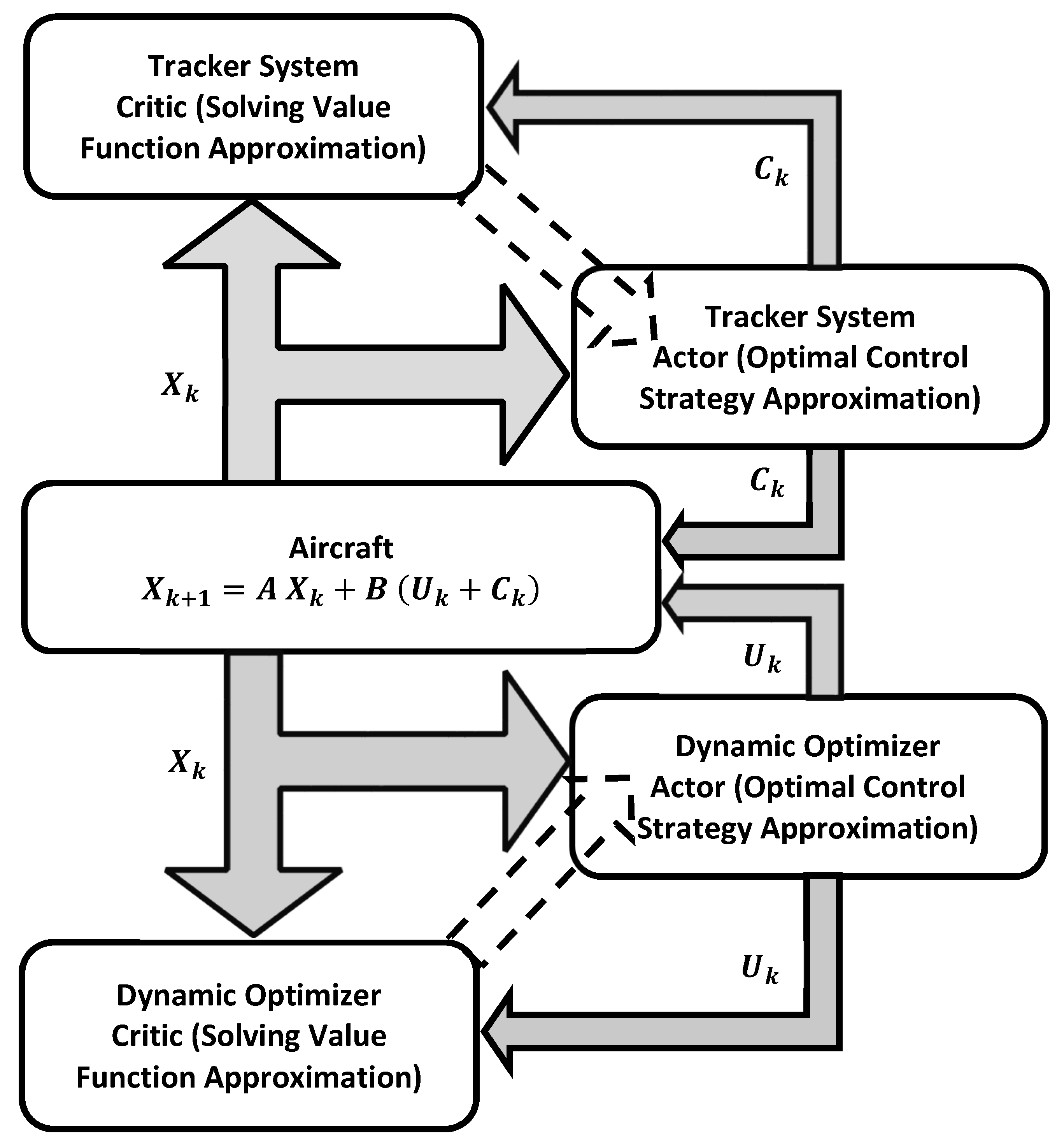
The adaptive critics approaches are employed to advise various neural network solutions for optimal control problems. They implement two-step reinforcement learning processes using separate neural network approximation schemes. The solution for Bellman optimality equation or the Hamilton–Jacobi–Bellman equation is implemented using a feedforward neural structure described by the critic structure. On the other hand, the optimal control strategy is approximated using an additional feedforward neural network structure called the actor structure. The update processes of the actor and critic weights are interactive and coupled in the sense that the actor weights are tuned when the critic weights are updated following reward/punish assessments of the dynamic learning environment [28,30,33,37,40]. The sequences of the actor and critic weights-updates follow those advised by the respective value or policy iteration algorithms [28,37]. Reinforcement learning solutions are implemented in continuous-time platforms as well as discrete-time platforms, where integral forms of Bellman equations are used [55,56]. These structures are applied to multi-agent systems as well as single-agent systems, where each agent has its own actor-critic structure [34,35]. The adaptive critics are employed to provide neural network solutions for the dual heuristic dynamic programming problems for multi-agent systems [19,20]. These structures solve the underlying graphical games in a distributed fashion where the neighbor information is used. Actor-critic solution implementation for an optimal control problem with nonlinear cost function is introduced in [55]. The adaptive critics implementations for feedback control systems are highlighted in [57]. A PD scheme is combined with a reinforcement learning mechanism to control the tip-deflection and trajectory-tracking operation of a two-link flexible manipulator in [58]. The adopted actor-critic learning structure compensates for the variations in the payload. An adaptive trajectory-tracking control approach based on actor-critic neural networks is developed for a fully autonomous underwater vehicle in [59]. The nonlinearities in the control input signals are compensated for during the adaptive control process.

This work contributions are four-fold:

• An online control mechanism is developed to solve the tracking problem in uncertain dynamical environment without acquiring any knowledge about the dynamical models of the underlying systems.
• An innovative temporal difference solution is developed using a reformulation of Bellman optimality equation. This form does not require existence of admissible initial policies and it is computationally simple and easy to apply.
• The developed learning approach solves the tracking problem for each dynamical process using separate interactive linear feedback control laws. These optimize the tracking as well as the overall dynamical behavior.
• The outcomes of the proposed architecture can be generalized smoothly for structured dynamical problems. Since, the learning approach is suitable for discrete-time control environments and it is applicable for complex coupled dynamical problems.

The paper is structured as follows: Section 2 is dedicated to the formulation of the optimal tracking control problem along with the model-free temporal difference solution forms. Model-free adaptive learning processes are developed in Section 3, and their real-time adaptive critics or neural network implementations are presented in Section 4. Digital simulation outcomes for an autonomous controller of a flexible wing aircraft are analyzed in Section 5. The implications of the developed machine learning processes in practical applications and some future research directions are highlighted in Section 6. Finally, concluding remarks about the adaptive learning mechanisms are presented in Section 7.

2. Formulation of the Optimal Tracking Control Problem

Optimal tracking control theory is used to lay out the mathematical foundation of various adaptive learning solution frameworks. Thus, many adaptive mechanisms employ complicated control strategies which are difficult to implement in discrete-time solution environments. In addition, many tracking control schemes are model-dependent, which raises concerns about their performances in unstructured dynamical environments [17]. This section tackles these challenges by mapping the optimization objectives of underlying tracking problem using machine learning solution tools.

2.1. Combined Optimization Mechanism

The optimal tracking control problem, in terms of the operation, can be divided broadly into two main objectives [17]. The first is concerned with asymptotically stabilizing the tracking error dynamics of the system, and the second optimizes the overall energy during the tracking process. Herein, the outcomes of the online adaptive learning processes are two linear feedback control laws. The adaptive approach uses simple linear quadratic utility or cost functions to evaluate the real-time optimal control strategies. The proposed approach tackles many challenges associated with the traditional tracking problems [17]. First, it allows an online model-free mechanism to solve the tracking control problem. Second, it allows several flexible tracking control configurations which are adaptable with the complexity of the dynamical systems. Finally, it allows interactive adaptations for both the tracker and optimizer feedback control laws.

The learning approach does not employ any information about the dynamics of the underlying system. The selected online measurements can be represented symbolically using the following form

$$X_{k+1}=F(X_k,U_k),$$

(1)

where $X\in {\mathbb{R}}^{n\times 1}$ is a vector of selected measurements (i.e., the sufficient or observable online measurements), $U\in {\mathbb{R}}^{m\times 1}$ is a vector of control signals, k is a discrete-time index, and F represents the model that generates the online measurements of the dynamical system which could retain linear or nonlinear representations.

The tracking segment of the overall tracking control scheme generates the optimal tracking control signal $C_{k\left\{i\right\}}\in \mathbb{R}\forall k$ using a linear feedback control law that depends on the sequence of tracking errors $e_{k\left\{i\right\}},e_{k-1\left\{i\right\}},e_{k-2\left\{i\right\}},$ where each error signal $e_{k\left\{i\right\}}$ is associated with the $i^{th}$ state or measured variable of vector $X_k$ (i.e., $X_{k\left\{i\right\}}$). The error $e_{k\left\{i\right\}}$ is defined by $e_{k\left\{i\right\}}=T_{k\left\{i\right\}}-X_{k\left\{i\right\}},$ where $T_{k\left\{i\right\}}$ is the reference signal of the state or measured variable $X_{k\left\{i\right\}}$. On one side, the number of online tracking control loops is determined by the number of reference variables or states. Each reference signal $T_{k\left\{i\right\}}$ has a tracking evaluation loop. In this development, a feedback control law that uses combination of three errors (i.e., $e_{k\left\{i\right\}},e_{k-1\left\{i\right\}},e_{k-2\left\{i\right\}}$) is considered in order to mimic the mechanism of a Proportional-Integral-Derivative (PID) controller in discrete-time where the tracking gains are adapted in real time in an online fashion. On the other side, the form of each scalar tracking control law $C_{k\left\{i\right\}}$ can be formulated for any combinations of error samples (i.e., $e_{k\left\{i\right\}},e_{k-1\left\{i\right\}},e_{k-2\left\{i\right\}},e_{k-3\left\{i\right\}},\dots ,e_{k-N\left\{i\right\}}$). Thus, the proposed tracking structure enables higher-order difference schemes which can be realized smoothly in discrete-time environments. In order to simplify the tracking notations, $e_k$ and $C_k$ are used to refer to the tracking error signal $e_{k\left\{i\right\}}$ and tracking control signal $C_{k\left\{i\right\}}$ for each individual tracking loop respectively. Herein, each scalar actuating tracking control signal $C_{k\left\{i\right\}}$ simultaneously adjusts all relevant or applicable actuation control signals $U_{k\left\{j\right\}},j\in m$.

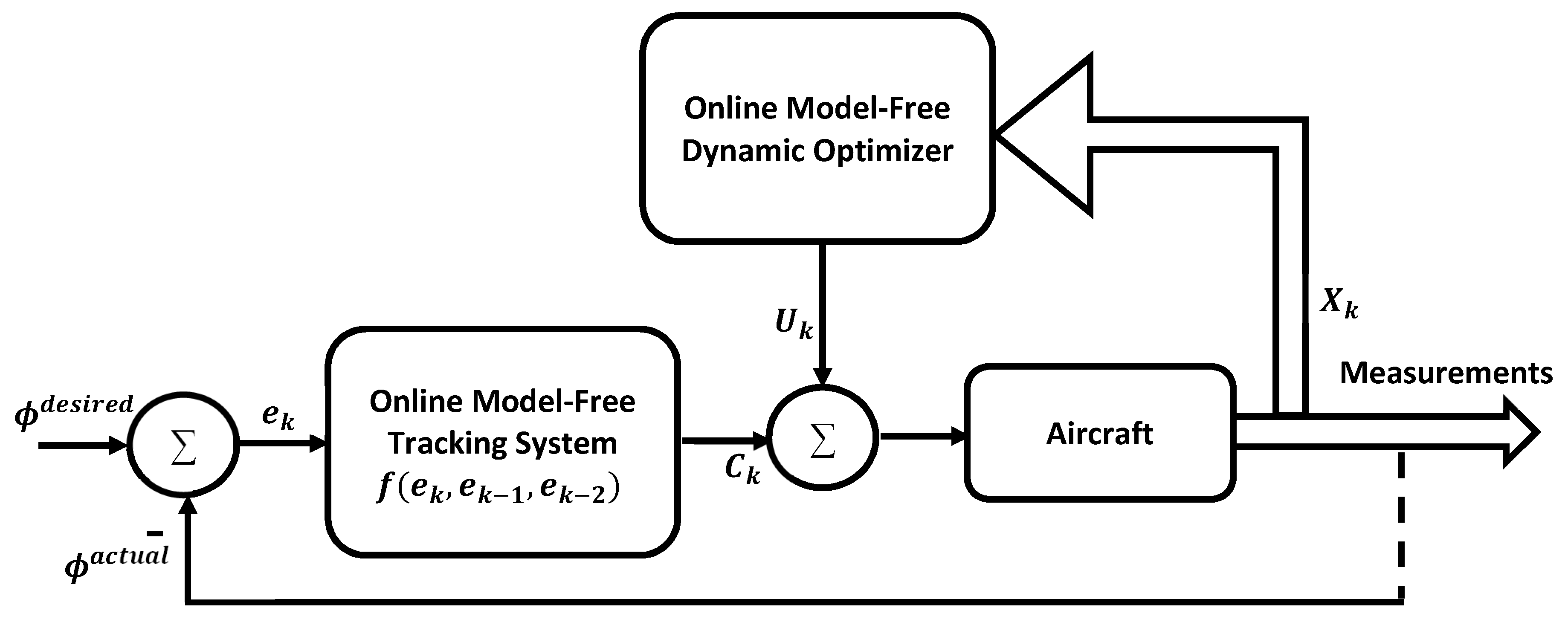
The overall layout of the control mechanism (i.e., considering the optimizing and tracking features) is sketched in Figure 1, where ${\varphi }^{desired}$ denotes a desired reference signal (i.e., each $T_{k\left\{i\right\}}$) and ${\varphi }^{actual}$ refers to the actual measured signal (i.e., each $X_{k\left\{i\right\}}$) for each individual tracking loop.

The goals of the optimization problem are to find the optimal linear feedback control laws or the optimal control signals $U_k^{*}$ and $C_k^{*}\forall k,$ using model-free machine learning schemes. The underlying objective utility functions are mapped into different temporal difference solution forms. As indicated above, since linear feedback control laws are used, then linear quadratic utility functions are employed to evaluate the optimality conditions in real time. The objectives of the optimization problem are detailed as follows:

(1) A measure index of the overall dynamical performance is minimized to calculate the optimal control signal $U_k^{*}$ such that

$$mi{n}_{U_k}O(X_k,U_k)$$

with linear quadratic objective cost function $O(X_k,U_k)=\frac{1}{2}\left(X_k^{T}Q{X}_k+U_k^{T}R{U}_k\right),$ where $Q\in {\mathbb{R}}^{n\times n}>\mathbf{0}$ and $R\in {\mathbb{R}}^{m\times m}>\mathbf{0}$ are symmetric positive definite matrices.

Therefore, the underlying performance index J is given by

$$J=\sum _{i=k}^{\infty }O\left(X_i,U_i\right).$$

(2) A tracking error index is optimized to evaluate the optimal tracking control signal $C_k^{*}$ such that

$$mi{n}_{C_k}D(E_k,C_k).$$

with an objective cost function $D(E_k,U_k)=\frac{1}{2}\left(E_k^{T}S{E}_k+C_k^{T}M{C}_k\right),$ where $E_k={\left[\begin{array}{ccc}{e}_k& e_{k-1}& e_{k-2}\end{array}\right]}^T,$ $S\in {\mathbb{R}}^{3\times 3}>\mathbf{0}$ is a symmetric positive definite matrix, and $M\in \mathbb{R}>\mathbf{0}$. The choice of the tracking error vector E is flexible to the number of the memorized tracking error signals $N_e$ such that $e_{k-\ell },\ell =0,1,\dots ,N_e$.

Therefore, the underlying performance index P is given by

$$P=\sum _{i=k}^{\infty }D\left(E_i,C_i\right).$$

Herein, the choice of the optimized policy structure $U_k^{*}$ to be a function of the states $X_k$ is not meant to achieve asymptotic stability in a standalone operation (i.e., all the states $X_k,\forall k$ go to zero). Instead, it is incorporated into the overall control architecture where it can select the minimum energy path during the tracking process. Hence, it creates an asymptotically stable performance around the desired reference trajectory. Later, the performance of the standalone tracker is contrasted against that of the combined tracking control scheme to highlight this energy exchange minimization outcome.

2.2. Optimal Control Formulation

Various optimal control formulations of the tracking problem promote multiple temporal difference solution frameworks [17,18]. These use Bellman equations or Hamilton–Jacobi–Bellman structures or even gradient forms of Bellman optimality equations [19,20,35]. The manner at which the cost or objective function is selected plays a crucial role in forming the underlying temporal difference solution and hence its associated optimal control strategy form. This work provides a generalizable machine learning solution framework, where the optimal control solutions are found by solving the underlying Bellman optimality equations of the dynamical systems. These can be implemented using policy iteration approaches with model-based schemes. However, these processes necessitate having initial admissible policies, which is essential to ensure admissibility of the future policies. This is further faced by computational limitations, for example, the reliance of the solutions on least square approaches with possible singularities-related calculation risks. This urged for flexible developments such as online value iteration processes where they do not encounter these problems.

Value iteration processes based on two temporal difference solution forms are developed to solve the tracking control problem. These are equivalent to solving the underlying Hamilton–Jacobi–Bellman equation of the optimal tracking control problem [17,46]. Regarding the problem under consideration, it is required to have two temporal difference equations: One solves for the optimal control strategies to minimize the tracking efforts, and the other selects the supporting control signals to minimize the energy exchanges during the tracking process. In order to do that, two solving value functions related to the main objectives, are proposed such that

$$\mathsf{\Gamma }\left(X_k,U_k\right)=J=\sum _{i=k}^{\infty }O\left(X_i,U_i\right),$$

where $\mathsf{\Gamma }(\dots )$ is a solving value function that approximates the overall minimized dynamical performance and it is defined by

$$\begin{array}{c}\hfill {\displaystyle \mathsf{\Gamma }\left(X_k,U_k\right)=\frac{1}{2}\left[X_k^{\mathrm{T}}{U}_k^{\mathrm{T}}\right]H\left[\begin{array}{c}{X}_k\hfill \\ U_k\hfill \end{array}\right],H=\left[\begin{array}{cc}{H}_{XX}\hfill & H_{XU}\hfill \\ H_{UX}\hfill & H_{UU}\hfill \end{array}\right].}\end{array}$$

Similarly, the solving value function that approximates the optimal tracking performance is given by

$$\mathsf{\Xi }\left(E_k,C_k\right)=P=\sum _{i=k}^{\infty }D\left(E_i,C_i\right),$$

where ${\displaystyle \mathsf{\Xi }\left(E_k,C_k\right)=\frac{1}{2}\left[E_k^{\mathrm{T}}{C}_k^{\mathrm{T}}\right]\mathsf{\Pi }\left[\begin{array}{c}{E}_k\hfill \\ C_k\hfill \end{array}\right],H=\left[\begin{array}{cc}{\mathsf{\Pi }}_{EE}\hfill & {\mathsf{\Pi }}_{EC}\hfill \\ {\mathsf{\Pi }}_{CE}\hfill & {\mathsf{\Pi }}_{CC}\hfill \end{array}\right].}$

These performance indices yield the following Bellman or temporal difference equations

$$\mathsf{\Gamma }\left(X_k,U_k\right)=\frac{1}{2}\left(X_k^{T}Q{X}_k+U_k^{T}R{U}_k\right)+\mathsf{\Gamma }\left(X_{k+1},U_{k+1}\right),$$

(2)

and

$$\mathsf{\Xi }\left(E_k,C_k\right)=\frac{1}{2}\left(E_k^{T}S{E}_k+C_k^{T}M{C}_k\right)+\mathsf{\Xi }\left(E_{k+1},C_{k+1}\right).$$

(3)

where the optimal control strategies associated with both Bellman equations are calculated as follows

$$U_k^{*}=argmi{n}_{U_k}\mathsf{\Gamma }\left(X_k,U_k\right)\to H_{UX}{X}_k+H_{UU}{U}_k^{*}=0.$$

Therefore, the optimal policy for the overall optimized performance is given by

$$U_k^{*}=-H_{UU}^{-1}{H}_{UX}{X}_k.$$

(4)

In a similar fashion, the optimal tracking control strategy is calculated using

$$C_k^{*}=argmi{n}_{C_k}\mathsf{\Xi }\left(E_k,C_k\right)\to {\mathsf{\Pi }}_{CE}{E}_k+{\mathsf{\Pi }}_{CC}{U}_k^{*}=0.$$

Therefore, the optimal policy for the optimized tracking performance is given by

$$C_k^{*}=-{\mathsf{\Pi }}_{CC}^{-1}{\mathsf{\Pi }}_{CE}{E}_k.$$

(5)

Using the optimal policies (4) and (5) into Bellman Equations (2) and (3) respectively yields the following Bellman optimality equations or temporal difference equations

$${\mathsf{\Gamma }}^{*}\left(X_k,U_k^{*}\right)=\frac{1}{2}\left(X_k^{T}Q{X}_k+U_k^{*T}R{U}_k^{*}\right)+{\mathsf{\Gamma }}^{*}\left(X_{k+1},U_{k+1}^{*}\right),$$

(6)

and

$${\mathsf{\Xi }}^{*}\left(E_k,C_k^{*}\right)=\frac{1}{2}\left(E_k^{T}S{E}_k+C_k^{*T}M{C}_k^{*}\right)+{\mathsf{\Xi }}^{*}\left(E_{k+1},C_{k+1}^{*}\right).$$

(7)

where ${\mathsf{\Gamma }}^{*}(\dots )$ and ${\mathsf{\Xi }}^{*}(\dots )$ are the optimal solutions for the above Bellman optimality equations

Solving Bellman optimality Equations (6) or (7) is equivalent to solving the underlying Hamilton–Jacobi–Bellman equations of the optimal tracking control problem.

Remark 1.

Model-free value iteration processes employ temporal difference solution forms that arise directly from Bellman optimality Equations (6) or (7), in order to solve the proposed optimal tracking control problem. This learning platform shows how to enable Action-Dependent Heuristic Dynamic Programming (ADHDP) solution, a class of approximate dynamic programming that employs a solving value function that is dependent on a state-action structure, in order to solve the optimal tracking problem in an online fashion [37,60].

3. Online Model-Free Adaptive Learning Processes

Bellman optimality Equations (6) and (7) are used to develop online value iteration processes. Herein, two adaptive learning algorithms are developed using these optimality equations. They share the ability to produce control strategies while they learn the dynamic environment in real time and the strategies do not depend on the dynamical model of the system under consideration.

3.1. Direct Value Iteration Process

The first model-free value iteration algorithm (Algorithm 1) uses direct forms of (6) and (7) as follows:

Algorithm 1 Model-free direct value iteration process.

Initialize ${\mathsf{\Gamma }}^0(X_0,U_0),{\mathsf{\Xi }}^0(E_0,C_0),U_0^0$ and $C_0^0$.     Update the solving value functions $\mathsf{\Gamma }(\dots )$ and $\mathsf{\Xi }(\dots )$ using $$\begin{array}{ccc}\hfill {\mathsf{\Gamma }}^{r+1}\left(X_k,U_k\right)& =& O^r\left(X_k,U_k\right)+{\mathsf{\Gamma }}^r\left(X_{k+1},U_{k+1}\right),\hfill \\ \hfill {\mathsf{\Xi }}^{r+1}\left(E_k,C_k\right)& =& D^r\left(E_k,C_k\right)+{\mathsf{\Xi }}^r\left(E_{k+1},C_{k+1}\right),\hfill \end{array}$$ (8) where r is an evaluation index.     Extract the optimal strategies $$\begin{array}{ccc}\hfill U_k^{r+1}& =& -{\left[H_{UU}^{-1}{H}_{UX}\right]}^{r+1}{X}_k,\hfill \\ C_k^{r+1}& =& -{\left[{\mathsf{\Pi }}_{CC}^{-1}{\mathsf{\Pi }}_{CE}\right]}^{r+1}{E}_k.\end{array}$$ (9) Terminate the updates of the solving value functions when $\parallel H^{r+1}(..)-H^r(..)\parallel \le \epsilon$ and $\parallel {\mathsf{\Pi }}^{r+1}(..)-{\mathsf{\Pi }}^r(..)\parallel \le \epsilon$, $\epsilon$ is an error threshold.

3.2. Modified Value Iteration Process

Another adaptive learning algorithm based on an indirect value iteration process is proposed. This algorithm reformulates or modifies the way Bellman optimality equations are solved as follows;

$${\mathsf{\Gamma }}^{*}\left(X_k,U_k^{*}\right)-{\mathsf{\Gamma }}^{*}\left(X_{k+1},U_{k+1}^{*}\right)=\frac{1}{2}\left(X_k^{T}Q{X}_k+U_k^{*T}R{U}_k^{*}\right),$$

(10)

and

$${\mathsf{\Xi }}^{*}\left(E_k,C_k^{*}\right)-{\mathsf{\Xi }}^{*}\left(E_{k+1},C_{k+1}^{*}\right)=\frac{1}{2}\left(E_k^{T}S{E}_k+C_k^{*T}M{C}_k^{*}\right).$$

(11)

Therefore, a modified value iteration process based on these reformulations is structured in Algorithm 2 as follows

Algorithm 2 Modified model-free value iteration process.

Initialize ${\mathsf{\Gamma }}^0(X_0,U_0),{\mathsf{\Xi }}^0(E_0,C_0),U_0^0$ and $C_0^0$.     Update the solving value functions $\mathsf{\Gamma }(\dots )$ and $\mathsf{\Xi }(\dots )$ using $$\begin{array}{ccc}\hfill {\mathsf{\Gamma }}^{r+1}\left(X_k,U_k\right)-{\mathsf{\Gamma }}^{r+1}\left(X_{k+1},U_{k+1}\right)& =& O^r\left(X_k,U_k\right),\hfill \\ \hfill {\mathsf{\Xi }}^{r+1}\left(E_k,C_k\right)-{\mathsf{\Xi }}^{r+1}\left(E_{k+1},C_{k+1}\right)& =& D^r\left(E_k,C_k\right).\hfill \end{array}$$ (12) Extract the optimal strategies $$\begin{array}{ccc}\hfill U_k^{r+1}& =& -{\left[H_{UU}^{-1}{H}_{UX}\right]}^{r+1}{X}_k,\hfill \\ C_k^{r+1}& =& -{\left[{\mathsf{\Pi }}_{CC}^{-1}{\mathsf{\Pi }}_{CE}\right]}^{r+1}{E}_k.\end{array}$$ (13) Terminate the updates of the solving value functions when $\parallel H^{r+1}(..)-H^r(..)\parallel \le \epsilon$ and $\parallel {\mathsf{\Pi }}^{r+1}(..)-{\mathsf{\Pi }}^r(..)\parallel \le \epsilon$.

This value iteration process solves Bellman optimality equation in a way that does not require initial stabilizing policies and, unlike the policy iteration mechanisms, this solution framework does not imply any computational difficulties related to the evaluations of $\mathsf{\Gamma }(\dots )$ and $\mathsf{\Xi }(\dots )$ at the different evaluation steps.

The proposed value iteration processes optimize the overall dynamical performance towards the tracking objectives. This means that the two optimization objectives are interacting and coupled along the variables of interest. This is done in real time without acquiring any information about the dynamics of the underlying system.

3.3. Comparison to a Standard Policy Iteration Process

The value iteration process, as explained earlier, employs two steps, one is concerned with evaluating the optimal value function (i.e., solving Bellman optimality Equations (6) or (7)) and the second extracts the optimal policy given this value function (i.e., (4) or (5)). On the other hand, the policy iteration mechanism starts with a policy evaluation step that solves for a value function that is relevant to an attempted policy using Bellman equation (i.e., (2) or (3)) and this is followed by a policy improvement step that results in a strictly better policy compared to the preceding policy unless it is optimal [37,56,61].

To formulate a policy iteration process for the optimization problem in hand (i.e., the overall energy and tracking error minimization), the control signals $U^H$ and $C^{\mathsf{\Pi }}$ are evaluated using the linear policies $-\left[H_{UU}^{-1}{H}_{UX}\right]X$ and $-\left[{\mathsf{\Pi }}_{CC}^{-1}{\mathsf{\Pi }}_{CE}\right]E$, respectively, where the policy iteration process uses (2) and (3) repeatedly in order to perform a single-policy evaluation step, such that

$$\begin{array}{ccc}\hfill {\mathsf{\Gamma }}^j\left(X_k,U_k^H\right)-{\mathsf{\Gamma }}^j\left(X_{k+1},U_{k+1}^H\right)& =& O\left(X_k,U_k^H\right),\hfill \\ \hfill {\mathsf{\Xi }}^h\left(E_k,C_k^{\mathsf{\Pi }}\right)-{\mathsf{\Xi }}^h\left(E_{k+1},C_{k+1}^{\mathsf{\Pi }}\right)& =& D\left(E_k,C_k^{\mathsf{\Pi }}\right),\hfill \end{array}$$

where the symbols j and h refer to the calculation-instances leading to a policy evaluation step for each dynamical operation.

In other words, the solving value function $\mathsf{\Gamma }(\dots )$ is updated after collecting several necessary samples $\nu$ $\left(\mathrm{i}.\mathrm{e}.,{\tilde{Z}}_X^{j=1}(X_{k,k+1},U_{k,k+1}^H),\right.$ ${\tilde{Z}}_X^{j=2}(X_{k+1,k+2},U_{k+1,k+2}^H),$ $\dots ,$ $\left.{\tilde{Z}}_X^{j=\nu }(X_{k+\nu -1,k+\nu },U_{k+\nu -1,k+\nu }^H)\right),$ where $\nu =(n+m)\times (n+m+1)/2$ designates the number of entries of the upper/lower triangle block of matrix $H\in {\mathbb{R}}^{(n+m)\times (n+m)}$ and ${\tilde{Z}}_X$ is a vector associated with the vector transformation of the upper/lower triangle block of the symmetric matrix H [56,61]. This act lasts for at least a real-time interval of k to $k+\nu$ to collect sufficient information to fulfill the policy evaluation step [56,61]. Similarly, the solving value function $\mathsf{\Xi }\left(\dots \right)$ is updated at the end of each online interval k to $k+10$, where 10 samples (10 refers to the number of entries of the upper/lower triangle block of matrix $\mathsf{\Pi }\in {\mathbb{R}}^{4\times 4}$) are repeatedly collected in order to evaluate the taken tracking policy $\left(\mathrm{i}.\mathrm{e}.,{\tilde{Z}}_E^{h=1}(E_{k,k+1},C_{k,k+1}^{\mathsf{\Pi }}),\right.$ ${\tilde{Z}}_E^{h=2}(E_{k+1,k+2},C_{k+1,k+2}^{\mathsf{\Pi }}),$ $\dots ,$ $\left.{\tilde{Z}}_E^{h=10}(E_{k+9,k+10},C_{k+9,k+10}^{\mathsf{\Pi }})\right)$, where the vector ${\tilde{Z}}_E^h$ is structured in a similar manner as ${\tilde{Z}}_X$. The approach taken to construct vector ${\tilde{Z}}_X$ or ${\tilde{Z}}_E$ is detailed in [56,61]. The policy iteration solution results in a decreasing sequence of the solving value functions which is lower-bounded by zero.

The policy iteration process requires the existence of an initial admissible policy and could encounter mathematical risks when evaluating the underlying policies [56,61]. On the other hand, Algorithms 1 and 2 do not impose initial admissible policies and the optimal value functions $\mathsf{\Gamma }(\dots )$ and $\mathsf{\Xi }(\dots )$ are updated simultaneously at each real-time instance $r=k$, as explained by (8) and (12). The value iteration process retains simpler and flexible adaptation mechanism compared with the above policy iteration formulation, where the policy evaluation steps could exist at uncorrelated time-instances.

3.4. Convergence and Stability Results of the Adaptive Learning Mechanism

The convergence analysis and stability characteristics of the value iteration processes, based on action-dependent heuristic dynamic programming solution, are introduced for single and multi-agent systems and for continuous as well as discrete-time environments [20,35,60,62,63]. The adaptive learning value iteration processes result in non-decreasing sequences such that

$$\begin{array}{c}\hfill 0<\cdots \le {\mathsf{\Gamma }}^0\le {\mathsf{\Gamma }}^1\le {\mathsf{\Gamma }}^2\le \cdots \le {\mathsf{\Gamma }}^r\cdots \le {\mathsf{\Gamma }}^{*},\\ \hfill 0<\cdots \le {\mathsf{\Xi }}^0\le {\mathsf{\Xi }}^1\le {\mathsf{\Xi }}^2\le \cdots \le {\mathsf{\Xi }}^r\cdots \le {\mathsf{\Xi }}^{*},\end{array}$$

where ${\mathsf{\Gamma }}^{*}(\dots )$ and ${\mathsf{\Xi }}^{*}(\dots )$ are the upper bounded optimal solutions for Bellman optimality equations.

The sequences of the resultant control strategies $U_k^r,\forall k,r$ and $C_k^r,\forall k,r$ are stabilizing and hence admissible sequences. In a similar fashion, the following inequalities hold

$$\begin{array}{c}{\mathsf{\Gamma }}^r(X_k,U_k)-{\mathsf{\Gamma }}^r(X_{k+1},U_{k+1})\le {\mathsf{\Gamma }}^{r+1}(X_k,U_k)-{\mathsf{\Gamma }}^{r+1}(X_{k+1},U_{k+1}),\\ {\mathsf{\Xi }}^r(X_k,U_k)-{\mathsf{\Xi }}^r(X_{k+1},U_{k+1})\le {\mathsf{\Xi }}^{r+1}(X_k,U_k)-{\mathsf{\Xi }}^{r+1}(X_{k+1},U_{k+1}).\end{array}$$

The above inequalities are also bounded above using the same concepts adopted in [20,35,60,62,63]. The simulation results highlight the evolution of the solving value functions using Algorithms 1 and 2 in real time. Furthermore, they will judge the importance of Algorithm 2 in terms of the convergence speed and optimality of the solving value functions.

4. Neural Network Implementations

Adaptive critics are employed to implement the proposed adaptive learning solutions in real time. Each algorithm involves two steps. The first is concerned with solving a Bellman optimality equation, and the other approximates the optimal control strategy. Each step is implemented using a neural network approximation structure. The solving value function $\mathsf{\Gamma }(\dots )$ or $\mathsf{\Xi }(\dots )$ is approximated using a critic structure, while the associated optimal control policy is approximated using an actor structure. These represent coupled tuning processes with different objectives. The solving algorithms employ update processes to tune the critic weights, where they have different forms of the temporal difference equations. However, the way the actor is approximated for both adaptive algorithms is achieved in the same fashion. A full adaptive critics solution structure for the tracking control problem is shown in Figure 2.

4.1. Neural Network Implementation of Algorithm 1

The actor-critic adaptations for Algorithm 1 are done in real time using separate neural network structures as follows.

The solving value functions $\mathsf{\Gamma }(\dots )$ and $\mathsf{\Xi }(\dots )$ are approximated using the neural network structures

$$\widehat{\mathsf{\Gamma }}(.|{\mathsf{{\rm Y}}}_c)=\frac{1}{2}\left[X_k^T{\widehat{U}}_k^T\right]{\mathsf{{\rm Y}}}_c^{\mathrm{T}}\left[\begin{array}{c}{X}_k\hfill \\ {\widehat{U}}_k\hfill \end{array}\right]\mathrm{and}\widehat{\mathsf{\Xi }}(.|{\mathsf{\Omega }}_c)=\frac{1}{2}\left[E_k^T{\widehat{C}}_k^T\right]{\mathsf{\Omega }}_c^{\mathrm{T}}\left[\begin{array}{c}{E}_k\hfill \\ {\widehat{C}}_k\hfill \end{array}\right],$$

where ${\mathsf{{\rm Y}}}_c^T=\left[\begin{array}{cc}{\mathsf{{\rm Y}}}_{cXX}^T& {\mathsf{{\rm Y}}}_{cX\widehat{U}}^T\\ {\mathsf{{\rm Y}}}_{c\widehat{U}X}^T& {\mathsf{{\rm Y}}}_{c\widehat{U}\widehat{U}}^T\end{array}\right]\in {\mathbb{R}}^{(n+m)\times (n+m)}$ and ${\mathsf{\Omega }}_c^T=\left[\begin{array}{cc}{\mathsf{\Omega }}_{cEE}^T& {\mathsf{\Omega }}_{cE\widehat{C}}^T\\ {\mathsf{\Omega }}_{c\widehat{C}E}^T& {\mathsf{\Omega }}_{c\widehat{C}\widehat{C}}^T\end{array}\right]\in {\mathbb{R}}^{4\times 4}$ are the critic approximation weights matrices.

The optimal strategies $U^{*}$ and $C^{*}$ are approximated as

$${\widehat{U}}_k={\mathsf{{\rm Y}}}_a{X}_k\mathrm{and}{\widehat{C}}_k={\mathsf{\Omega }}_a{E}_k,$$

where ${\mathsf{{\rm Y}}}_a^T\in {\mathbb{R}}^{m\times 1}$ and ${\mathsf{\Omega }}_a^T\in {\mathbb{R}}^{3\times 1}$ are the approximation weights of the actors.

The tuning processes are interactive, and the weights of each structure are updated using a gradient descent approach. Therefore, the update laws for the critic weights for this algorithm are calculated as

$$\begin{array}{ccc}\hfill {\mathsf{{\rm Y}}}_c^{(r+1)T}& =& {\mathsf{{\rm Y}}}_c^{rT}-{\alpha }_c\left(\widehat{\mathsf{\Gamma }}(.|{\mathsf{{\rm Y}}}_c^{rT})-{\widehat{\mathsf{\Gamma }}}^{target}(.|{\mathsf{{\rm Y}}}_c^{rT})\right)Z_X{Z}_X^T,\hfill \\ \hfill {\mathsf{\Omega }}_c^{(r+1)T}& =& {\mathsf{\Omega }}_c^{rT}-{\alpha }_c\left(\widehat{\mathsf{\Xi }}(.|{\mathsf{\Omega }}_c^{rT})-{\widehat{\mathsf{\Xi }}}^{target}(.|{\mathsf{\Omega }}_c^{rT})\right)Z_E{Z}_E^T,\hfill \end{array}$$

(14)

where $0<{\alpha }_c<1$ is a critic learning rate, $Z_X=\left[\begin{array}{c}{X}_k\hfill \\ {\widehat{U}}_k^r\hfill \end{array}\right]$, $Z_E=\left[\begin{array}{c}{E}_k\hfill \\ {\widehat{C}}_k^r\hfill \end{array}\right],$ and the target values of the approximations ${\mathsf{\Gamma }}^{target}(\dots )$ and ${\mathsf{\Xi }}^{target}(\dots )$ are given by

$$\begin{array}{ccc}\hfill {\mathsf{\Gamma }}^{target}& =& O\left(X_k,{\widehat{U}}_k^r\right)+{\mathsf{\Gamma }}^r\left(X_{k+1},{\widehat{U}}_{k+1}^r\right),\hfill \\ \hfill {\mathsf{\Xi }}^{target}& =& D\left(E_k,{\widehat{C}}_k^r\right)+{\mathsf{\Pi }}^r\left(E_{k+1},{\widehat{C}}_{k+1}^r\right).\hfill \end{array}$$

In a similar fashion, the approximation weights of the optimal control strategies are updated using the rules

$$\begin{array}{ccc}\hfill {\mathsf{{\rm Y}}}_a^{(r+1)T}& =& {\mathsf{{\rm Y}}}_a^{rT}-{\alpha }_a{\left(\widehat{U}-{\widehat{U}}^{target}\right)}^r{X}_k^T,\hfill \\ \hfill {\mathsf{\Omega }}_a^{(r+1)T}& =& {\mathsf{\Omega }}_a^{rT}-{\alpha }_a{\left({\widehat{C}}_k-{\widehat{C}}_k^{target}\right)}^r{E}_k^T,\hfill \end{array}$$

(15)

where $0<{\alpha }_a<1$ defines the actor learning rate and the target values of the optimal policy approximations ${\widehat{U}}_k$ and ${\widehat{C}}_k$ are given by

$$\begin{array}{ccc}\hfill {\widehat{U}}^{target}& =& -{\left[{\mathsf{{\rm Y}}}_{c\widehat{U}\widehat{U}}^{-1}{\mathsf{{\rm Y}}}_{c\widehat{U}X}\right]}^r{X}_k,\hfill \\ \hfill {\widehat{C}}^{target}& =& -{\left[{\mathsf{\Omega }}_{c\widehat{C}\widehat{C}}^{-1}{\mathsf{\Omega }}_{c\widehat{C}E}\right]}^r{E}_k.\hfill \end{array}$$

Consequently, the critic and actor update laws are given by (14) and (15) respectively, where they form the implementation platforms of the solution steps (8) and (9) in Algorithm 1.

Remark 2.

The gradient descent approach employs actor-critic learning rates which take positive values less than 1. In the proposed development the actor-critic learning rates are tied to the sampling time used to generate the online measurements in the discrete-time environment. This is done to achieve smooth tuning for the actor-critic weights relative to the changes in the dynamics of the system. The gradient decent approaches do not have affirmative convergence criteria. However, as will be shown below, the simulation cases emphasize the usefulness of this approach even when a challenging dynamical environment is considered, where one of the challenging scenarios considers random actor-critic learning rates at each evaluation step in the real time processes.

4.2. Neural Network Implementation of Algorithm 2

The following development introduces the neural network implementations of the solution given by the modified value iteration solution presented by Algorithm 2.

The solving value function approximations $\tilde{\mathsf{\Gamma }}(.|{\Delta }_c)$ and $\tilde{\mathsf{\Xi }}(.|{\mathsf{\Lambda }}_c)$ are given by

$$\tilde{\mathsf{\Gamma }}(.|{\Delta }_c)=\frac{1}{2}\left[X_k^T{\tilde{U}}_k^T\right]{\Delta }_c^{\mathrm{T}}\left[\begin{array}{c}{X}_k\hfill \\ {\tilde{U}}_k\hfill \end{array}\right]\mathrm{and}\tilde{\mathsf{\Xi }}(.|{\mathsf{\Lambda }}_c)=\frac{1}{2}\left[E_k^T{\tilde{C}}_k^T\right]{\mathsf{\Lambda }}_c^{\mathrm{T}}\left[\begin{array}{c}{E}_k\hfill \\ {\tilde{C}}_k\hfill \end{array}\right],$$

where ${\Delta }_c^T=\left[\begin{array}{cc}{\Delta }_{cXX}^T& {\Delta }_{cX\tilde{U}}^T\\ {\Delta }_{c\tilde{U}X}^T& {\Delta }_{c\tilde{U}\tilde{U}}^T\end{array}\right]\in {\mathbb{R}}^{(n+m)\times (n+m)}$ and ${\mathsf{\Lambda }}_c^T=\left[\begin{array}{cc}{\mathsf{\Lambda }}_{cEE}^T& {\mathsf{\Lambda }}_{cE\tilde{C}}^T\\ {\mathsf{\Lambda }}_{c\tilde{C}E}^T& {\mathsf{\Lambda }}_{c\tilde{C}\tilde{C}}^T\end{array}\right]\in {\mathbb{R}}^{4\times 4}$ are the critic approximation weights matrices.

The approximations of the optimal control strategies $U^{*}$ and $C^{*}$ follow

$${\tilde{U}}_k={\Delta }_a{X}_k\mathrm{and}{\tilde{C}}_k={\mathsf{\Lambda }}_a{E}_k,$$

where ${\Delta }_a^T\in {\mathbb{R}}^{m\times 1}$ and ${\mathsf{\Lambda }}_a^T\in {\mathbb{R}}^{3\times 1}$ are the approximation weights of the actor neural network.

The tuning of the critic weights for both optimization loops follows

$$\begin{array}{ccc}\hfill {\overline{\Delta }}_c^{(r+1)T}& =& {\overline{\Delta }}_c^{rT}-{\eta }_c\left(\tilde{\mathsf{\Gamma }}(.|{\Delta }_c^{rT})-{\tilde{\mathsf{\Gamma }}}^{target}(.|{\Delta }_c^{rT})\right){\overline{Z}}_X^T,\hfill \\ \hfill {\overline{\mathsf{\Lambda }}}_c^{(r+1)T}& =& {\overline{\mathsf{\Lambda }}}_c^{rT}-{\eta }_c\left(\tilde{\mathsf{\Xi }}(.|{\mathsf{\Lambda }}_c^{rT})-{\tilde{\mathsf{\Xi }}}^{target}(.|{\mathsf{\Lambda }}_c^{rT})\right){\overline{Z}}_E^T,\hfill \end{array}$$

(16)

where $0<{\eta }_c<1$ is a critic learning rate, ${\overline{\Delta }}_c$ and ${\overline{\mathsf{\Lambda }}}_c$ are vector transformations of the upper triangle section of the symmetric solution matrices ${\Delta }_c$ and ${\mathsf{\Lambda }}_c$ respectively, ${\tilde{Z}}_X$ and ${\tilde{Z}}_E$ are the respective vector-to-vector transformations of ${\tau }_X^r$ and ${\tau }_E^r$ with ${\tau }_X^r=\left[\begin{array}{c}{X}_k\hfill \\ {\tilde{U}}_k^r\hfill \end{array}\right]-\left[\begin{array}{c}{X}_{k+1}\hfill \\ {\tilde{U}}_{k+1}^r\hfill \end{array}\right]$ and ${\tau }_E^r=\left[\begin{array}{c}{E}_k\hfill \\ {\tilde{C}}_k^r\hfill \end{array}\right]-\left[\begin{array}{c}{E}_{k+1}\hfill \\ {\tilde{C}}_{k+1}^r\hfill \end{array}\right]$.

The target values ${\tilde{\mathsf{\Gamma }}}^{target}(\dots )$ and ${\tilde{\mathsf{\Xi }}}^{target}(\dots )$ are calculated by

$$\begin{array}{ccc}\hfill {\tilde{\mathsf{\Gamma }}}^{target}& =& O\left(X_k,{\widehat{U}}_k^r\right),\hfill \\ \hfill {\tilde{\mathsf{\Xi }}}^{target}& =& D\left(E_k,{\widehat{C}}_k^r\right).\hfill \end{array}$$

The update of the actor weights for this solution algorithm follows a similar structure as of Algorithm 1 such that

$$\begin{array}{ccc}{\Delta }_a^{(r+1)T}\hfill & =& {\Delta }_a^{rT}-{\eta }_a{\left(\tilde{U}-{\tilde{U}}^{target}\right)}^r{X}_k^T,\hfill \\ {\mathsf{\Lambda }}_a^{(r+1)T}\hfill & =& {\mathsf{\Lambda }}_a^{rT}-{\eta }_a{\left({\tilde{C}}_k-{\tilde{C}}_k^{target}\right)}^r{E}_k^T,\hfill \end{array}$$

(17)

where $0<{\eta }_a<1$ is an actor learning rate, and the target values ${\tilde{U}}^{target}(\dots )$ and ${\tilde{C}}_k^{target}(\dots )$ are given by

$$\begin{array}{ccc}\hfill {\tilde{U}}^{target}& =& -{\left[{\Delta }_{c\tilde{U}\tilde{U}}^{-1}{\Delta }_{c\tilde{U}X}\right]}^r{X}_k,\hfill \\ \hfill {\tilde{C}}^{target}& =& -{\left[{\mathsf{\Lambda }}_{c\tilde{C}\tilde{C}}^{-1}{\mathsf{\Lambda }}_{c\tilde{C}E}\right]}^r{E}_k.\hfill \end{array}$$

5. Autonomous Flexible Wing Aircraft Controller

The proposed online adaptive learning approaches are employed to design an autonomous trajectory-tracking controller for a flexible wing aircraft. The flexible wing aircraft functions as a two-body system (i.e., the pilot/fuselage and wing systems) [10,13,14,15,16]. Unlike fixed wing systems, the flexible wing aircraft do not have exact aerodynamic models, due to the deformations in the wings which are continuously occurring [13,64,65]. Aerodynamic modeling attempts rely on semi-experimental results with no exact models, which complicated the autonomous control task and made it very challenging [13]. Recently, these aircraft have captured increasing attention to join the unmanned aerial vehicles family due to their low-cost operation features, uncomplicated design, and simple fabrication process [44]. The maneuvers are achieved by changing the relative centers of gravity between the pilot and wing systems. In order to change the orientation of the wing with respect to the pilot/fuselage system, the control bar of the aircraft takes different pitch-roll commands to achieve the desired trajectory. The pitch/roll maneuvers are achieved by applying directional forces on the control bar of the flexible wing system in order to create or alter the desired orientation of the wing with respect to the pilot/fuselage system [65,66].

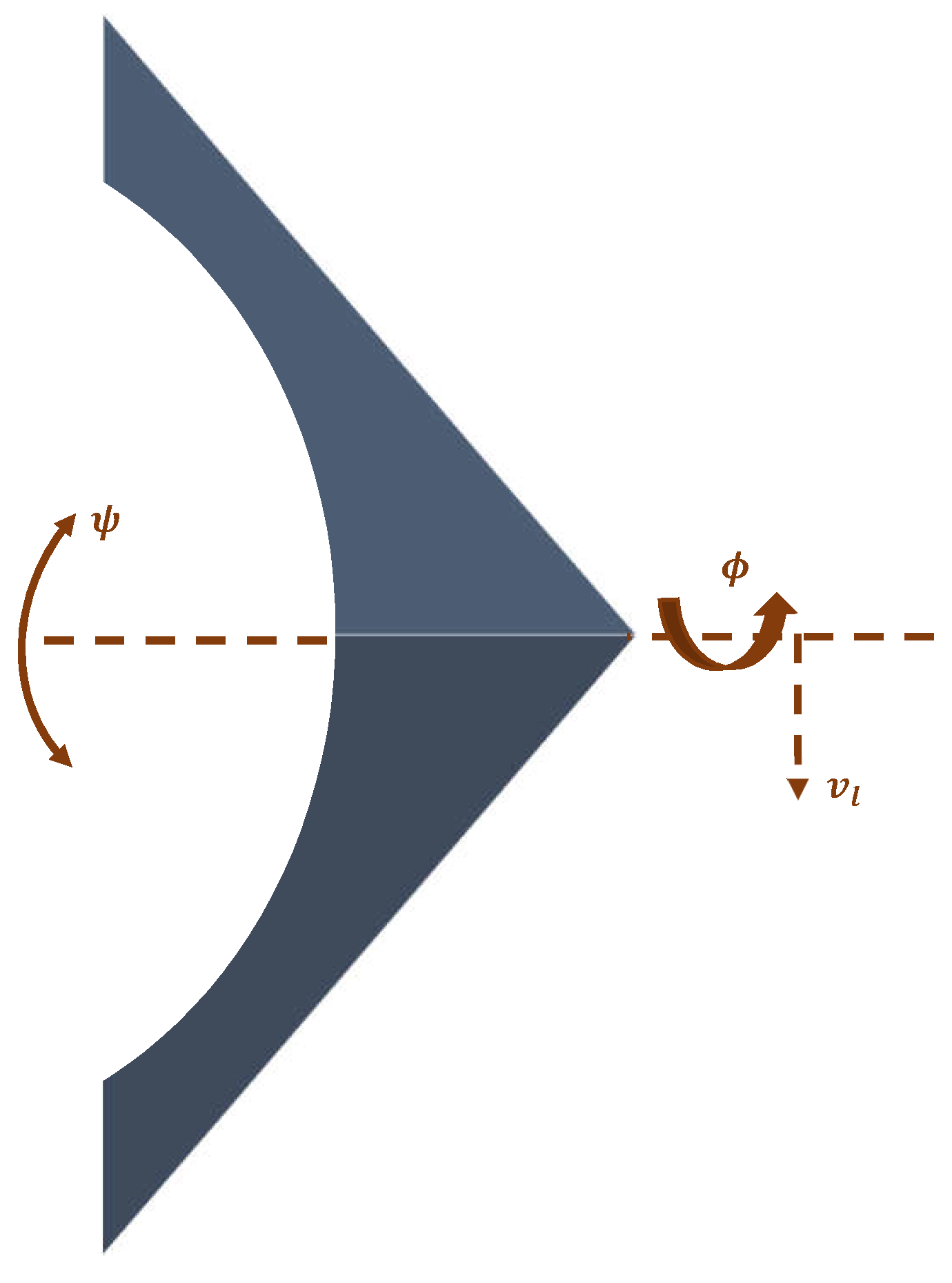
The objective of the autonomous aircraft controller design is to use the proposed online adaptive learning structures in order to achieve the roll-trajectory-tracking objectives, and to minimize energy paths (the dynamics of the aircraft) during the tracking process. The energy minimization is crucial for the economics of flying systems that share the same optimization objectives. The motions of the flexible wing aircraft are decoupled into longitudinal and lateral frames [13,64]. The lateral motion frame is hard to control compared to the inherited stability in the pitch motion frame. A lateral motion frame of a flexible wing aircraft is shown in Figure 3.

5.1. Assessment Criteria for the Adaptive Learning Algorithms

The effectiveness of the proposed online model-free adaptive learning mechanisms is assessed based on the following criteria:

• The convergence of the online adaptation processes (i.e., tuning of the actor and critic weights achieved using Algorithms 1 and 2). Consequently, the resulting trajectory-tracking error characteristics.
• The performance of the standalone tracking system versus the overall or combined tracking control scheme.
• The stability results of the online combined tracking control scheme (i.e., the aircraft is required to achieve the trajectory-tracking objective in addition to minimizing the energy exchanges during the tracking process).
• The benefits of the attempted adaptive learning approaches on improving the closed-loop time-characteristics of the aircraft during the navigation process.

Additionally, the simulation cases are designed to show how broadly Algorithm 2 (i.e., the newly modified Bellman temporal difference framework) will perform against Algorithm 1.

5.2. Generation of the Online Measurements

To apply the proposed adaptive approaches on the lateral motion frame, a simulation environment is needed to generate the online measurements. The different control methodologies do not use all the available measurements to control the aircraft [13,65]. Thus, the proposed approach is flexible to the selection of the key measurements. Hence, a lateral aerodynamic model at a trim speed, based on a semi-experimental study, is employed to generate the measurements as follows [13]

$$\begin{array}{c}\hfill X_{k+1}=A{X}_k+B{U}_{Tk},\end{array}$$

where the lateral state vector of the wing system is given by $X={\begin{array}{ccccc}\hfill [v_l& \dot{\varphi }& \dot{\psi }\hfill & \varphi & \psi ]\end{array}}^T$ and $U_T$ is the lateral control signal applied to the control bar.

The control signal $U_T$ is the overall combined control strategy decided by the tracker system and the optimizer system (i.e., $U_{Tk}=U_k+C_k$). In this example, the banking control signal aggregates dynamically the scalar signals $U_k\in \mathbb{R}$ and $C_k\in \mathbb{R}$ in real time in order to get an equivalent control signal $U_{Tk}$ that is applied to the control bar in order to optimize the motion following a trajectory-tracking command. The optimizer will decide the state feedback control policy $U_k=f\left(X_k\right)$ using the measurements $X_k$, where the linear state feedback optimizer control gains ${\mathsf{\Omega }}_a,{\mathsf{\Lambda }}_a\in {\mathbb{R}}^{1\times 5}$ are decided by the proposed adaptive learning algorithms. Similarly, the tracking system will decide the linear tracking feedback control policy $C_k$ based on the error signals $(e_k,e_{k-1},e_{k-2})$, where $e_k={\varphi }_k^{desired}-{\varphi }_k^{actual},\forall k$. The linear feedback tracking control gains ${\mathsf{{\rm Y}}}_a,{\Delta }_a\in {\mathbb{R}}^{1\times 3}$ are adapted in real time using the online reinforcement learning algorithms.

Noticeably, the proposed online learning solutions do not employ any information about the dynamics (i.e., drift dynamics A and control input matrix B), where they function like black-box mechanisms. Moreover, the control objectives are implemented in an online fashion, where only real-time measurements are considered. In other words, the control mechanism for the roll maneuver generates the real-time control strategy for the roll motion frame regardless what is occurring in the pitch direction and vice versa.

5.3. Simulation Environment

As described earlier, a state space model captured at a trim flight condition is used to generate online measurements [13]. A sampling time of $T_s=0.001$, creates the discrete-time state space matrices

$$A=\left[\begin{array}{rrrrr}0.9998& -0.0002& -0.0108& 0.0097& -0.0013\\ -0.0015& 0.9789& 0.0074& 0& 0\\ 0.0003& 0.0037& 0.9979& 0& 0\\ 0& 0.0010& 0& 1.0000& 0\\ 0& 0& 0.0010& 0& 1.0000\end{array}\right],B=\left[\begin{array}{c}\hfill 0\\ \hfill 0.0036\\ \hfill 0.0004\\ \hfill 0\\ \hfill 0\end{array}\right].$$

The learning parameters for the adaptive learning algorithms are given by ${\eta }_a={\eta }_c={\alpha }_a={\alpha }_c=0.0001$. The learning parameters are selected to be comparable to the sampling time to have smooth adjustments for the adapted weights. Later, random learning rates are superimposed at each evaluation step.

The initial conditions are set to $X_0={\begin{array}{ccccc}\hfill [40& 1.6& 0.8\hfill & -0.8& 0.2]\end{array}}^T.$

The weighting matrices of the cost functions $D(\dots )$ and $E(\dots )$ are selected in such a way as to normalize the effects of the different variables in order to increase the sensitivity of the proposed approach against the variations in the measured variables. These are given by $S=0.0001I_{3\times 3}$, $M=0.0001$, $R=907$, $Q=\left[\begin{array}{ccccc}0.0625& 0& 0& 0& 0\\ 0& 25& 0& 0& 0\\ 0& 0& 25& 0& 0\\ 0& 0& 0& 100& 0\\ 0& 0& 0& 0& 100\end{array}\right].$

The desired roll-tracking trajectory consists of two smooth opposite turns represented by a sinusoidal reference signal such that ${\varphi }^{desired}\left(t\right)=25sin(2\pi t/10)deg$ (i.e., right and left turns with max amplitudes of $25deg$).

5.4. Simulation Outcomes

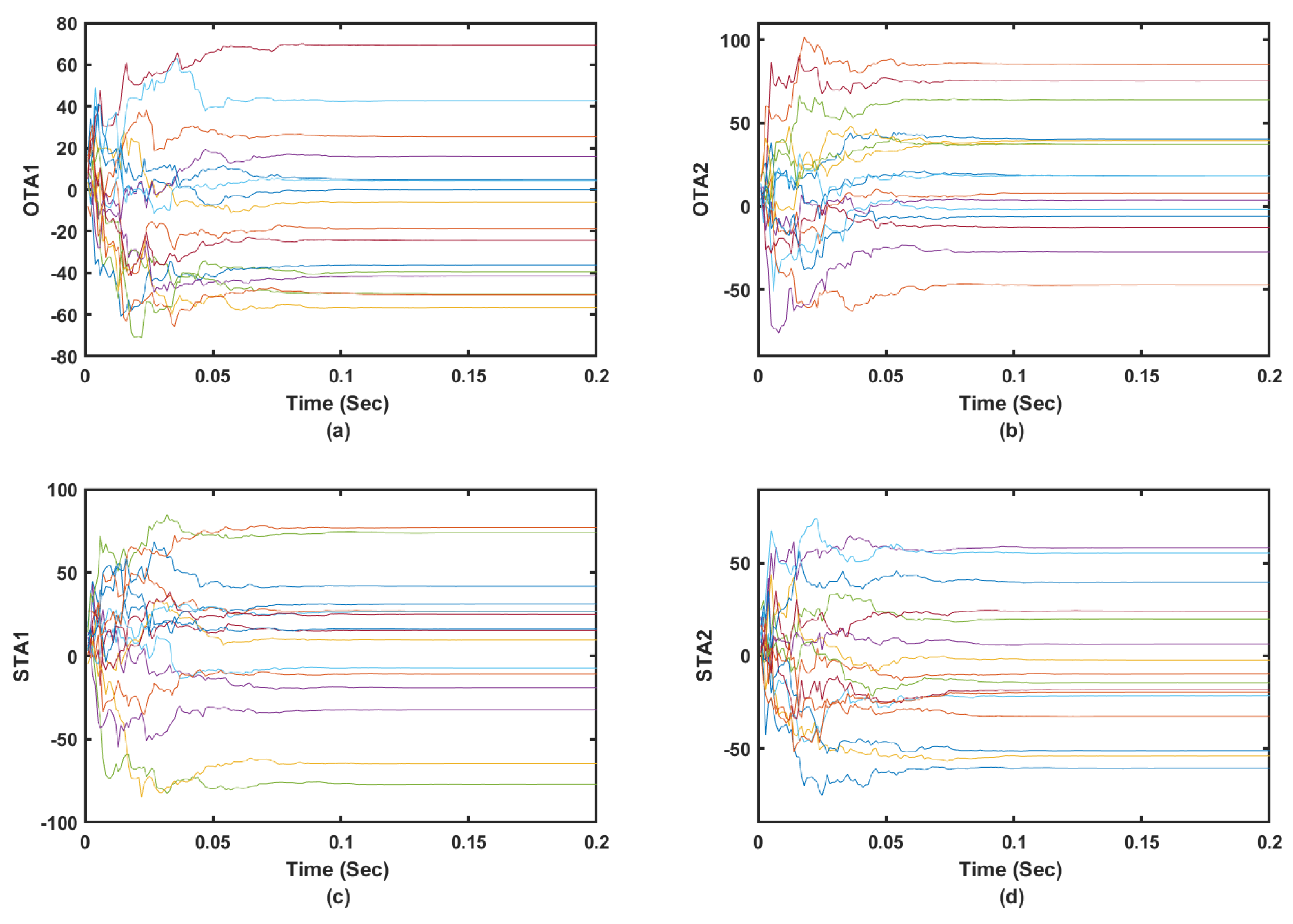
The simulation scenarios tackle the performance of the standalone tracker, then the characteristics of the overall or combined adaptive control approach. Finally, a third scenario is considered to discuss the performance of the adaptive learning algorithms under unstructured dynamical environment and uncertain learning parameters. These simulation cases can be detailed out as follows

• Standalone tracker: The adaptive learning algorithms are tested to achieve only the trajectory-tracking objective (i.e., no overall dynamical optimization is included, and they are denoted by STA1 and STA2 for Algorithms 1 and 2 respectively). In the standalone tracking operation mode, Bellman equations concerning the optimized overall performance and hence the associated optimal control strategies are omitted form the overall adaptive learning structure.
• Combined control scheme: This case combines the adaptive tracking control and optimizer schemes (i.e., the tracking control objective is considered along with the overall dynamical optimization using Algorithms 1 and 2 which are referred to as OTA1 and OTA2 respectively).
• Operation under uncertain dynamical and learning environments: The proposed online reinforcement learning approaches are validated using challenging dynamical environment, where the dynamics of the aircraft (i.e., matrices A and B) are allowed to variate at each evaluation step by $\pm 50\%$ around their nominal values at a normal trim condition. The aircraft is allowed to follow a complicated trajectory to highlight the capabilities of the adaptive learning processes using this maneuver. Additionally, the actor-critic learning rates are allowed to variate at each iteration index or solution step.

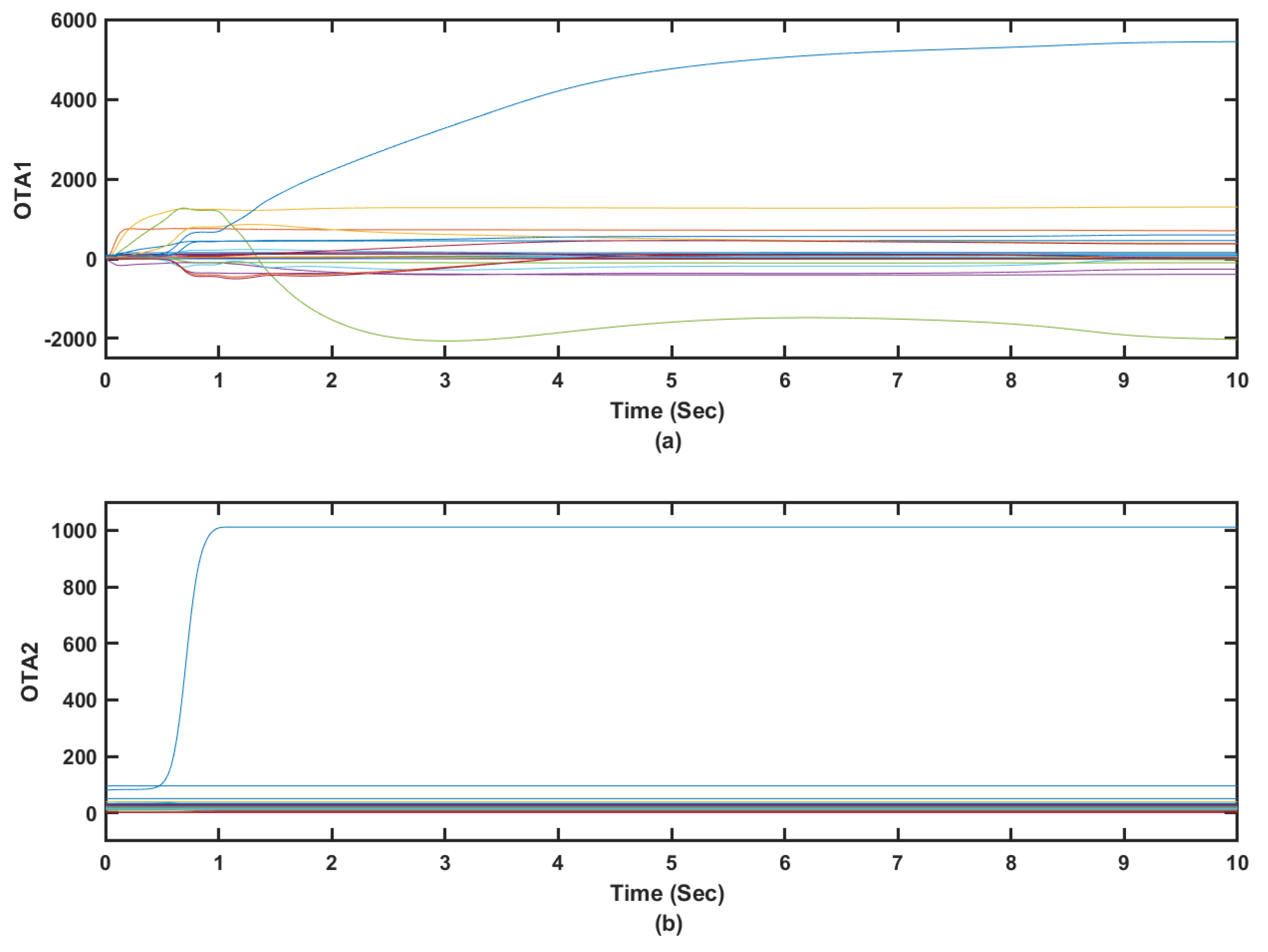
5.4.1. Adaptation of the Actor-Critic Weights

The tuning processes of the actor and critic weights are shown to converge when they follow solution Algorithms 1 and 2 as shown in Figure 4, Figure 5 and Figure 6. This is noticed when the tracker is used in a standalone situation or when it is operated within the combined or overall dynamical optimizer. It is shown that the actor and critic weights for the tracking component of the optimization process converge in less than $0.1$ s as shown in Figure 4 and Figure 5. The tuning of the critic weights in the case of optimized tracker took longer time due to the number of involved states and the objective of the overall dynamical optimization problem as shown in Figure 6. It is worth noting that the tracker part of the controller uses the tracking error signals as inputs which facilitates the tracking optimization process. These results highlight the capability of the adaptive learning algorithms to converge in real time.

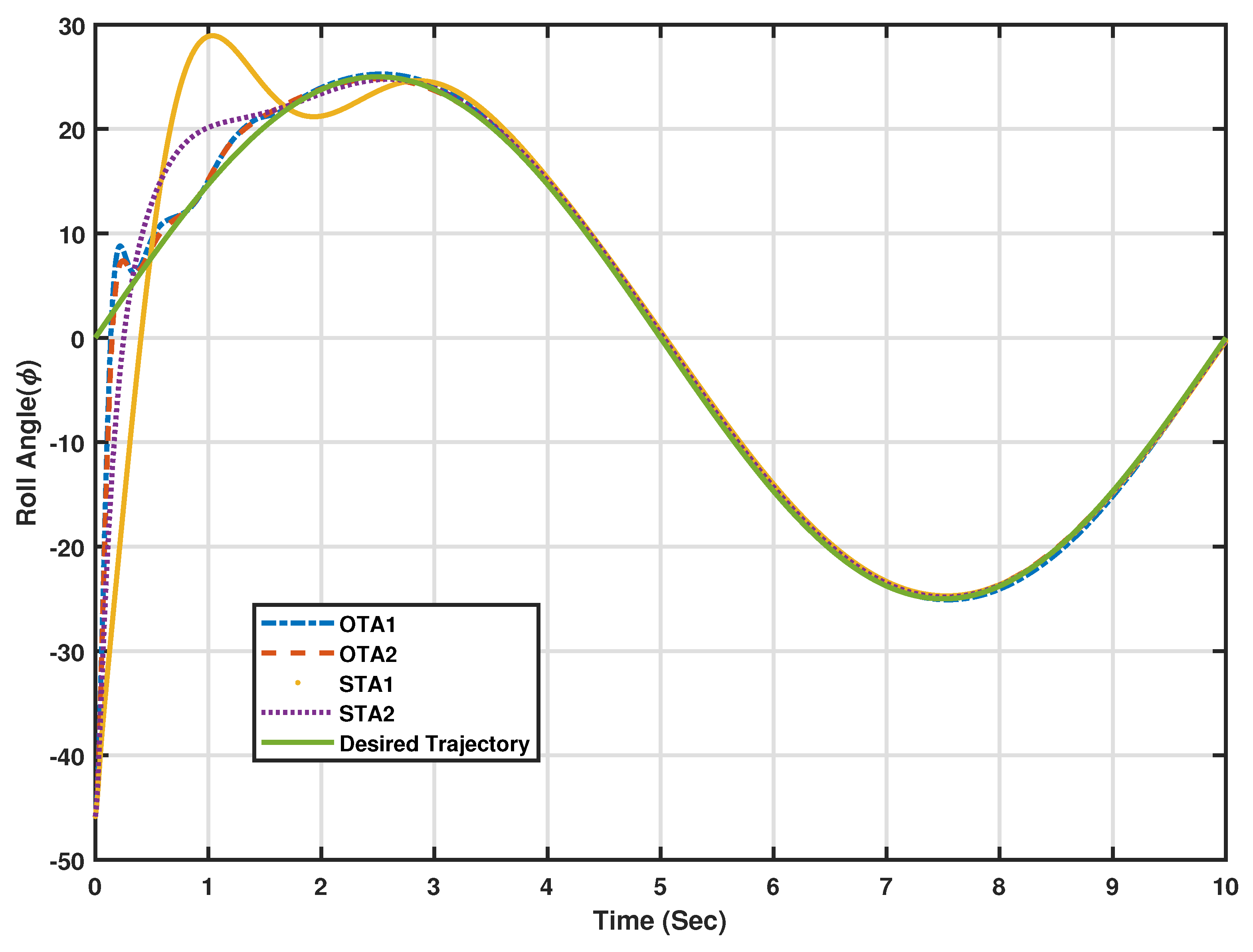
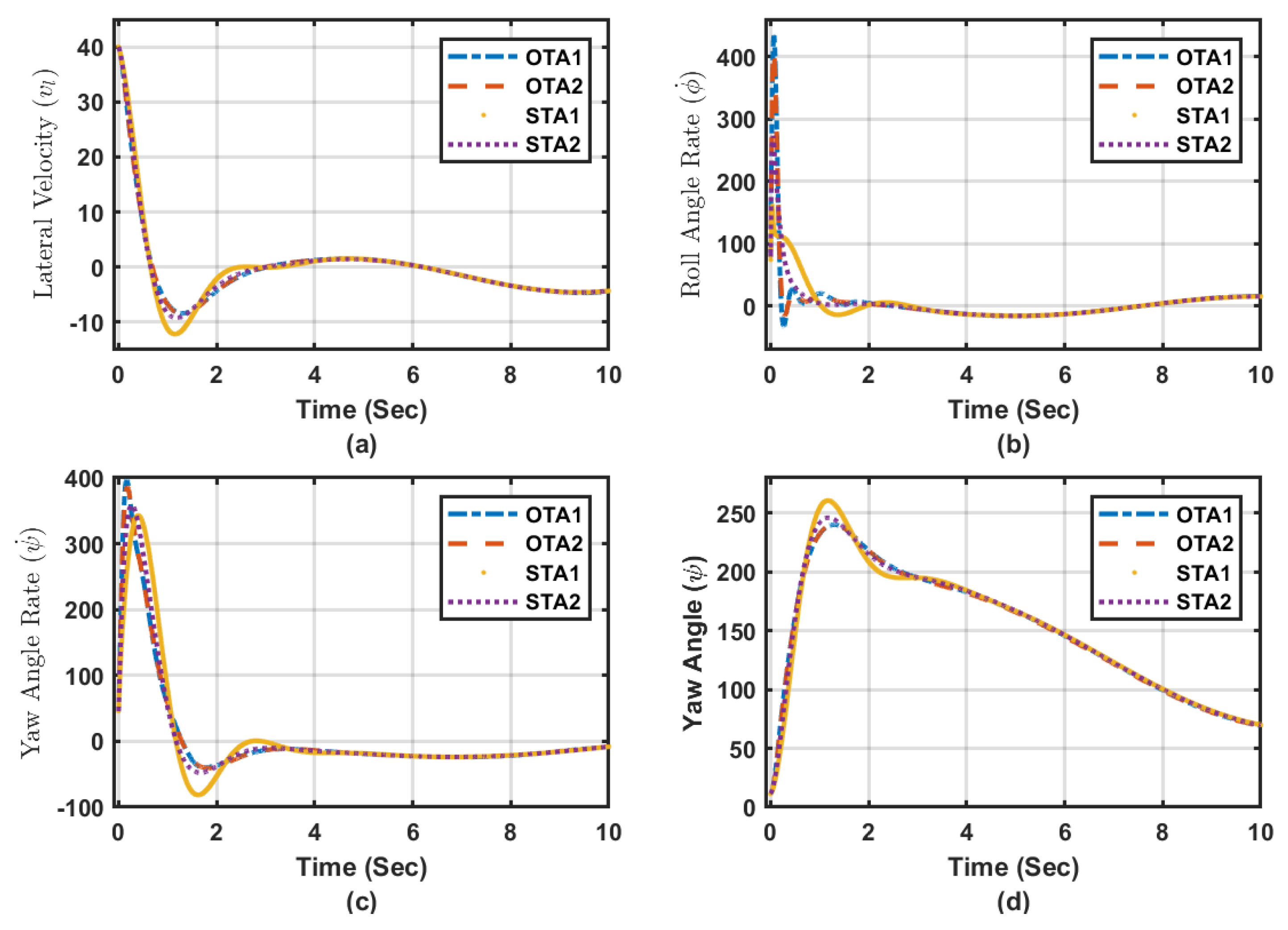
5.4.2. Stability and Tracking Error Measures

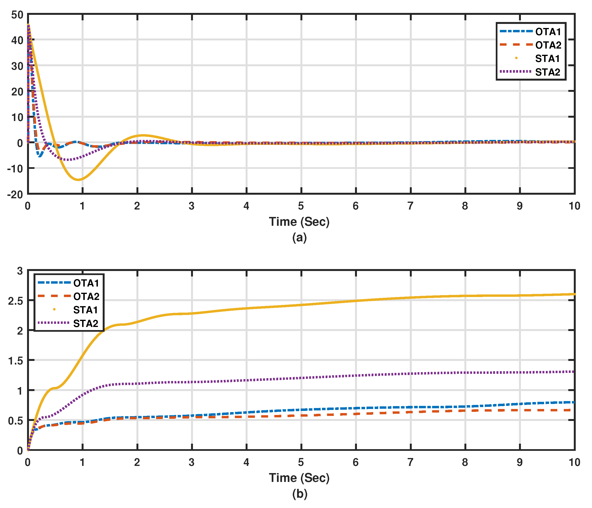
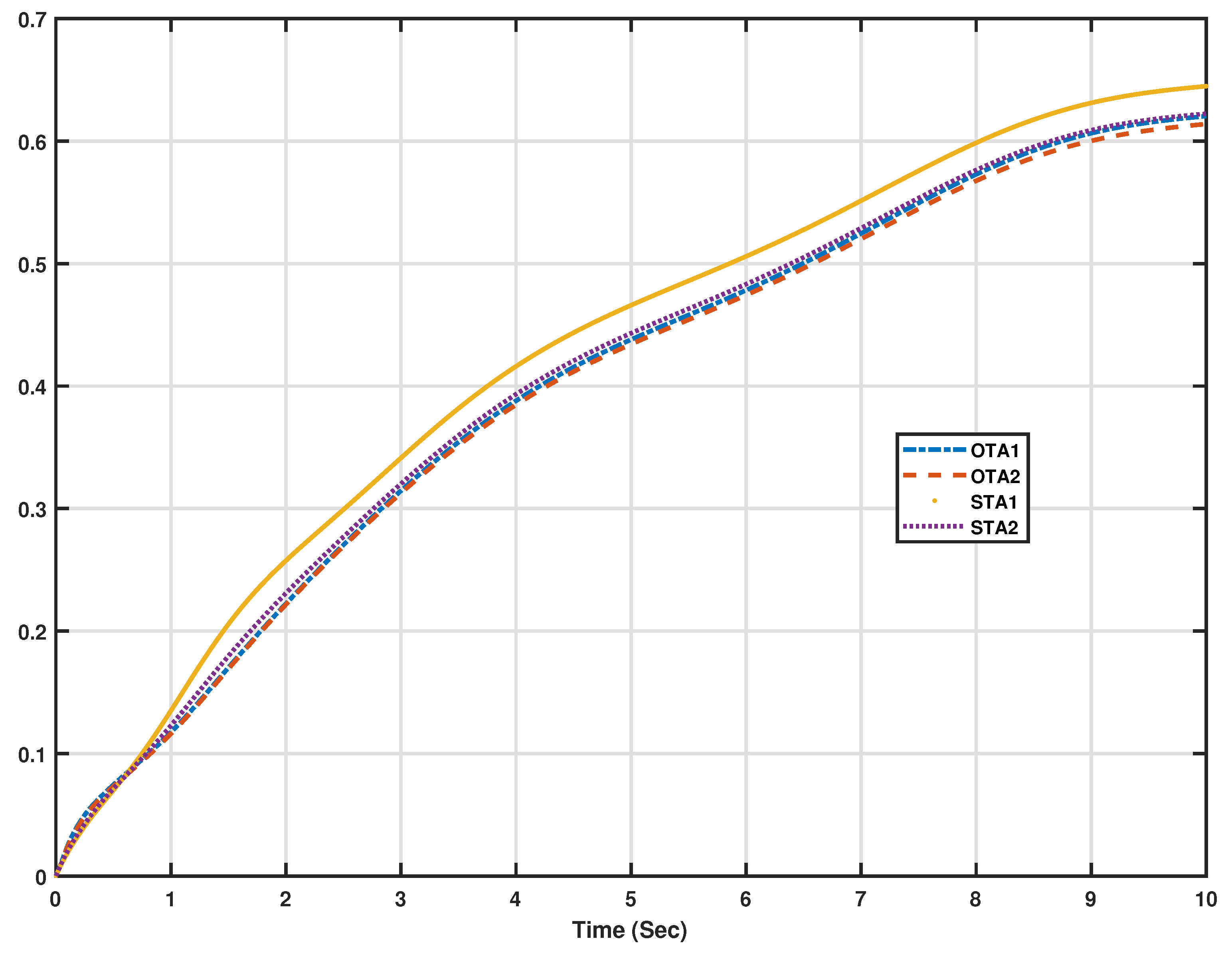
The adaptive learning algorithms under different scenarios or modes of operation, stabilize the flexible wing system along the desired trajectory as shown in Figure 7 and Figure 8. The lateral motion dynamics eventually follow the desired trajectory. In this case, the lateral variables are not supposed to decay to zero, since the aircraft is following a desired trajectory. The tracking scheme leads this process side by side with the overall energy optimization process, which actually improves the closed-loop characteristics of the aircraft towards minimal energy behavior. It is noticed that Algorithm 2 outperforms Algorithm 1 under standalone tracking mode or the overall optimized tracking mode. In order to quantify these effects numerically and graphically, the average accumulated tracking errors obtained using the proposed adaptive learning algorithms are shown in Figure 9a,b respectively. These indicate that the optimized tracker modes of operation (i.e., OTA1 and OTA2) give lower errors compared to those achieved during the standalone modes of operations (i.e., STA1 and STA2), emphasizing the importance of adding the overall optimization scheme to the tracking system. Adaptive learning Algorithm 2, using the optimized tracking mode, achieves the lowest average of accumulated errors as shown in Figure 9b. An additional measure index is used, where the overall normalized dynamical effects are evaluated using the following Normalized Accumulated Cost Index (NACI)

$$\mathrm{NACI}=\frac{1}{N}\sum _{k=0}^{10sec}\left[X_k^T{U}_{Tk}^T\right]\left[\begin{array}{cc}{V}_1& 0\\ 0& V_2\end{array}\right]\left[\begin{array}{c}{X}_k\hfill \\ U_{Tk}\hfill \end{array}\right],$$

where $V_1=\left[\begin{array}{ccccc}0.0006& 0& 0& 0& 0\\ 0& 0.0174& 0& 0& 0\\ 0& 0& 0.0208& 0& 0\\ 0& 0& 0& 1.5625& 0\\ 0& 0& 0& 0& 0.0483\end{array}\right],$ $V_2=0.2268,$ and $N=10,000$ (i.e., the number of iterations during 10 s) is the total number of samples.

The normalization values are the square of the maximum measured values of $X_k$ and $U_{Tk}$. The adaptive algorithm (OTA2) achieves the lowest overall dynamical cost or effort as shown by Figure 10. The final control laws achieved by using the different algorithms under the above modes of operation (i.e., STA1, STA2, OTA1, and OTA2) are listed in

Table 1. Final control laws.

Method	Control Law
${\mathsf{\Omega }}_a$ (STA1)	$\begin{array}{ccc}\hfill [57.5021& -1.1475& -26.1183]\hfill \end{array}$
${\mathsf{\Lambda }}_a$ (STA2)	$\begin{array}{ccc}\hfill [95.3475& -47.6060& 3.5581]\hfill \end{array}$
${\mathsf{\Omega }}_a$ (OTA1)	$\begin{array}{ccc}\hfill [81.2142& 13.2197& 16.6757]\hfill \end{array}$
${\mathsf{\Lambda }}_a$ (OTA2)	$\begin{array}{ccc}\hfill [70.8768& 23.9006& 3.0130]\hfill \end{array}$
${\mathsf{{\rm Y}}}_a$ (OTA1)	$\begin{array}{ccccc}\hfill [-0.0535& -0.0897& -0.1386\hfill & -0.3704& -0.3545]\end{array}$
${\Delta }_a$ (OTA2)	$\begin{array}{ccccc}\hfill [-0.0422& -0.1487& -0.3479\hfill & -0.4356& -0.1217]\end{array}$

.

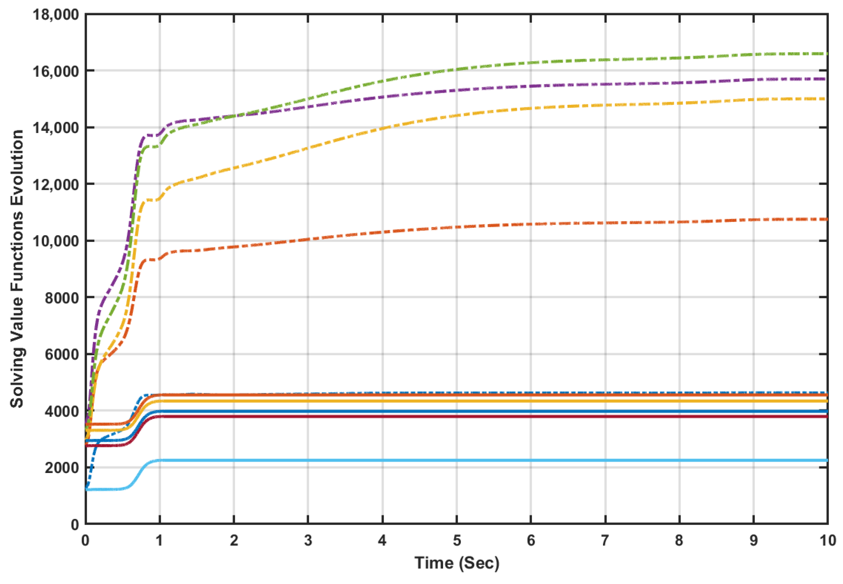
The online value iteration processes result in increasing bounded sequences of the solving value functions ${\mathsf{\Gamma }}^r(\dots )$ and ${\mathsf{\Xi }}^r(\dots ),\forall r$, which is aligned with the convergence properties of typical value iteration mechanisms. The online learning outcomes of the value iteration processes ${\mathsf{\Gamma }}^r(\dots )$ (i.e., using Algorithms 1 and 2) are applied and used for five random initial conditions as shown by Figure 11. The initial solving value functions evaluated by Algorithms 1 and 2 start from the same positions using the same vector of initial conditions. It is observed that Algorithm 2 (solid lines) outperforms Algorithm 1 (dashed lines) in terms of the updated solving value function obtained using the attempted random initial conditions. Despite both algorithms show general increasing and converging evolution pattern of the solving value functions, value iteration Algorithm 2 exhibits rapid increment and quicker settlement to lower values compared to Algorithm 1.

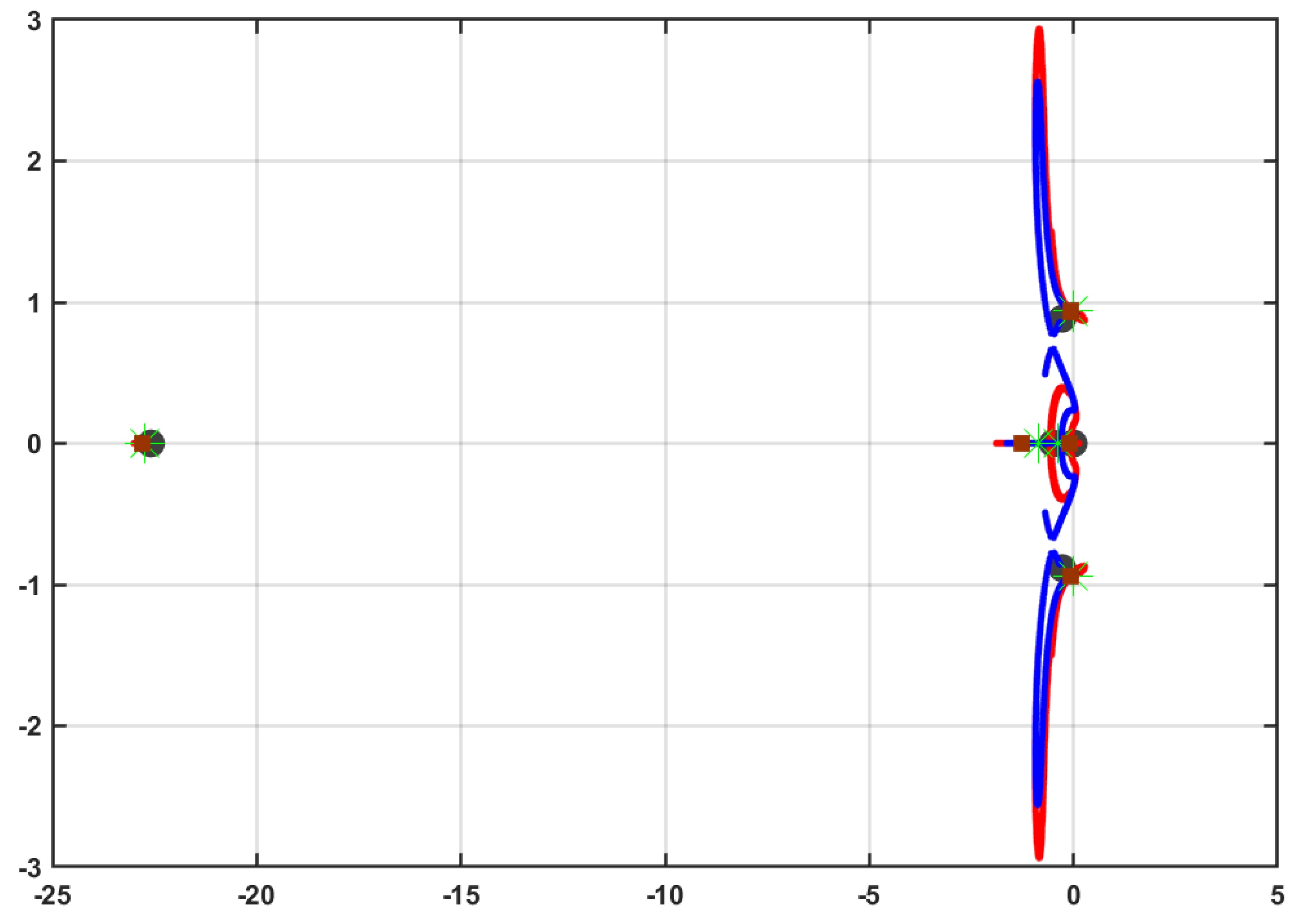
5.4.3. Closed-Loop Characteristics

To examine the time-characteristics of the adaptive learning algorithms, the closed-loop performances of the adaptive learning algorithms under the optimized tracking operation mode (i.e., OTA1 and OTA2) are plotted in Figure 12. Apart from the tracking feedback control laws, the optimizer state feedback control laws directly affect the closed-loop system. The forthcoming analysis is to show how (1) the aircraft system initially starts (i.e., open-loop system); (2) the evolution of the closed-loop poles during the learning process; and (3) the final closed-loop characteristics when the actor weights finally converge. The trace of the closed-loop poles achieved using OTA2 (i.e., the ● marks) shows concise and faster stable behavior than that obtained using OTA1 (i.e., the ● indicators), and definitely faster than the open-loop characteristics. The dominant open-loop pole is moved further into the stability region, when the overall dynamical optimizer is included, as listed in

Table 2. Open- and closed-loop eigenvalues.

Method	Poles
Open-loop system	$0,-0.2752\pm 0.8834i,$
(STA1 and STA2)	$-0.5088,-22.5902$
Closed-loop system	$-0.0169\pm 0.9393i,$
(OTA1)	$-0.3771,-0.8736,-22.7489$
Closed-loop system	$-0.0768\pm 0.9409i,$
(OTA2)	$-0.1152,-1.2600,-22.8079$

. These results emphasize the stability and superior time-response characteristics achieved using the adaptive learning approaches, especially Algorithm 2.

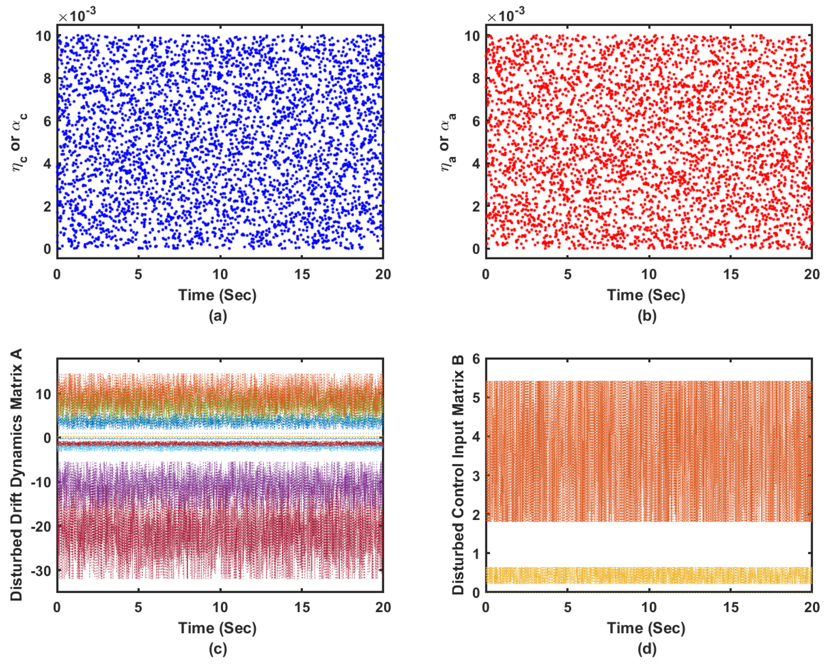
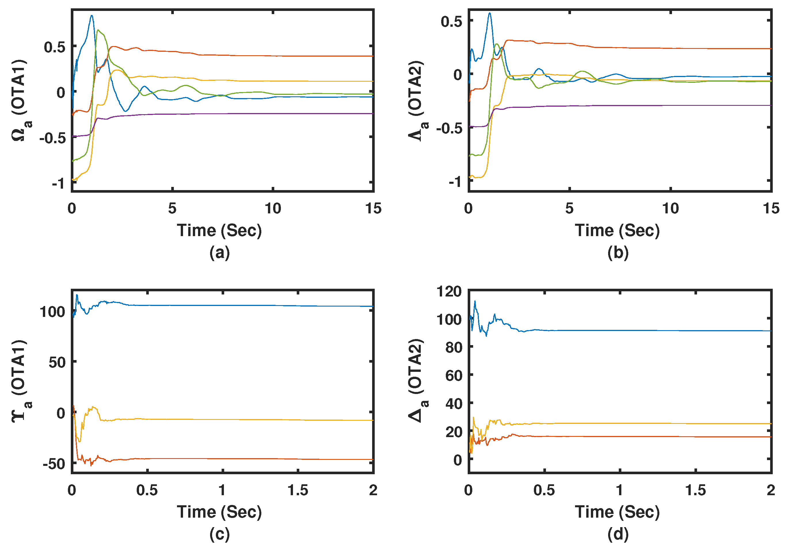
5.4.4. Performance in Uncertain Dynamical Environment

This simulation scenario challenges the performance of the online adaptive controller in uncertain dynamical environment. The continuous-time aircraft aerodynamic model (i.e., the aircraft state space model with the drift dynamics matrix A and control input matrix B) is forced to involve unstructured dynamics [13]. These disturbances are of amplitudes $\pm 50\%$ around the nominal values at the trim condition and they are generated from a normal Gaussian distribution as shown in Figure 13c,d. Additionally, the sampling time is set to $T_s=0.005$ s and the actor-critic learning rates are allowed to vary at each evaluation step as shown by Figure 13a,b to test a band of learning parameters. Finally, a challenging desired trajectory is proposed such that ${\varphi }^{desired}\left(t\right)=(25sin(6\pi t/10)+15cos(16\pi t/10))e^{-3t/10}deg$. These coexisting factors challenge the effectiveness of the controller. The randomness which appears in the proposed coexisting dynamical learning situations provides rich exploration environment for the adaptive learning processes. These dynamic variations occur at each evaluation step which guarantees some sort of generalization for the dynamical processes under consideration.

Figure 14a–d emphasize that the adaptive learning Algorithms 1 and 2 (i.e., OTA1 and OTA2) are able to achieve the trajectory-tracking objectives. The actor weights are shown to successfully converge despite the co-occurring uncertainties. The adaptation processes are effectively responding to the acting disturbances, where relatively longer time is needed to converge to the proper control gains. 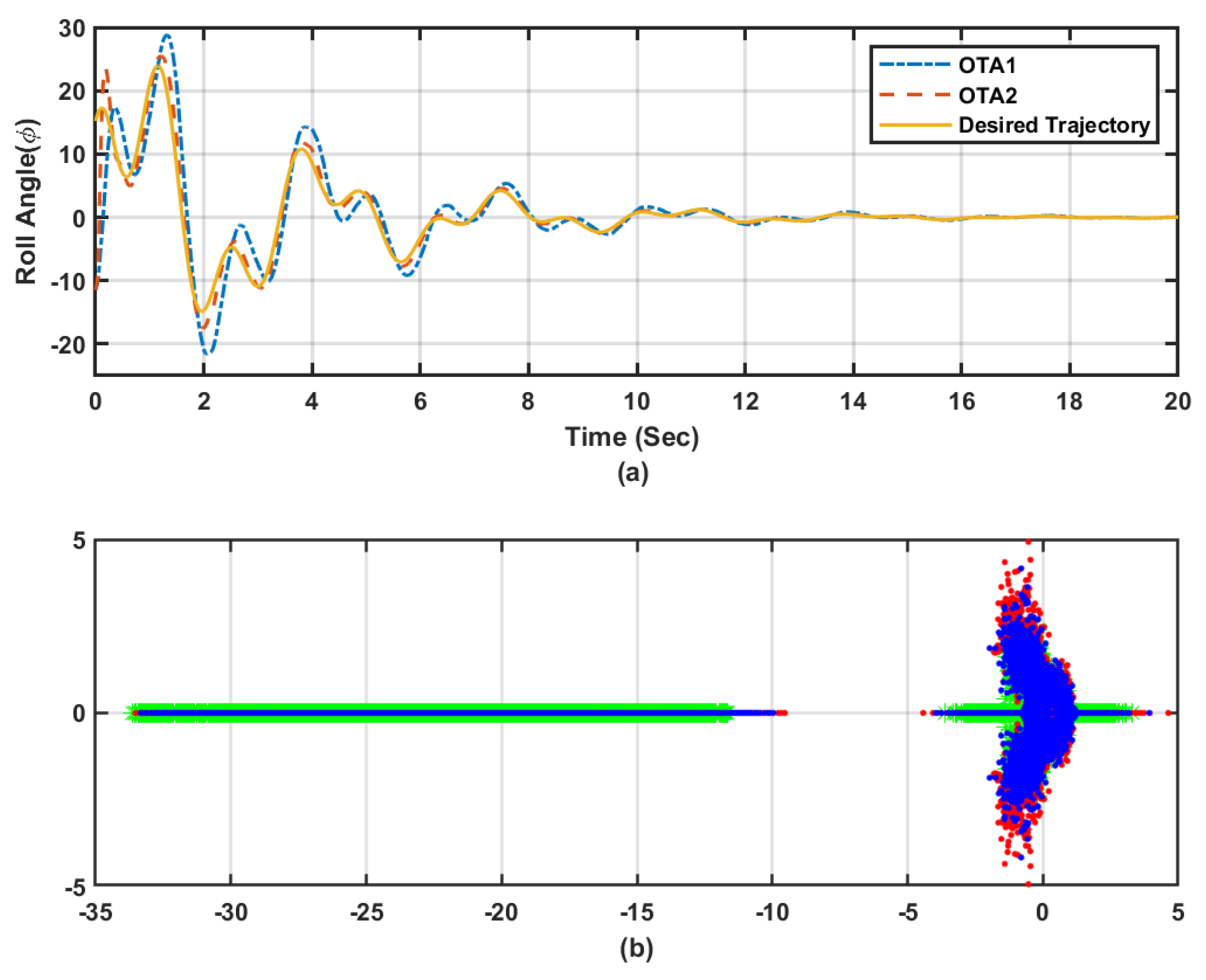The tracking feedback control gains took shorter time to converge as shown by Figure 14c,d, where the tracking feedback control law depends only on the state ${\varphi }_k$, and implicitly its derivative. Algorithm 2 exhibited better trajectory-tracking features compared to those obtained using Algorithm 1 as shown by Figure 15a. Figure 15b, when compared to Figure 12, shows how the open-loop poles, represented by ❋ marks (recorded disturbances at each iteration k), spread all over the S-plane. The adaptive learning Algorithms 1 and 2, exhibited similar stable behavior as observed in the earlier scenarios. However, longer time was needed to reach asymptotic stability around the desired reference trajectory. This can be observed by examining the spread of the closed-loop poles obtained using OTA1 (● notations) and OTA2 (● symbols). These results highlight the insensitivity of the proposed adaptive learning approaches against different uncertainties in the dynamic learning environments.

6. Implications in Practical Applications and Future Research Developments

The proposed combined adaptive learning approach can be integrated into various complex robotic or nonlinear system applications using extremely flexible adaptive learning black-box mechanisms. These are keen to optimize the performance of the actuation devices while maintaining the tracking control mission in an online fashion. At least, it will enable complicated distributed tracking solutions for structured robotic systems using simple adaptation laws with affordable computational costs compared to existing adaptive approaches. It can work in unstructured dynamical enthronements where it is really difficult to have full dynamical models for the underlying systems. The proposed adaptive learning algorithms can be deployed directly into the control units, where the only precautions are concerned with; (1) matching the sampling frequency (imposed by the sensory devices) to the learning parameters; (2) conditioning the weighting matrices in the utility or cost functions according to the actuation signals and the measured variables. The proposed learning approach is adaptive to the selection of the measured states which makes it convenient to use in many real-world applications, since it does not rely on complicated adaptive learning constraints.

Future research directions may extend other reinforcement learning tools, such as policy iteration schemes, in order to develop combined adaptive tracking processes. This direction should find means to tackle the admissibility requirements of the initial policies along with relaxing the computational efforts required to accomplish these processes. The proposed adaptive learning approaches can be adopted for multi-agent applications. Taking into consideration the complexity of the multi-agent structures, this would involve further research investigations which tackle connectivity, communication costs, and stabilizability of the coupled control schemes as well as the convergence conditions for the adaptive learning solutions. These ideas may consider structures based on Bellman equations as well as the Hamilton–Jacobi–Bellman equations. Additional directions may investigate the use of other approximate dynamic programming classes which employ gradient-based solving forms to solve the optimal tracking control problem [17,37]. These involve solutions for the Dual Heuristic Dynamic Programming and Action-Dependent Dual Heuristic Dynamic Programming problems. These developments should handle the dependence of the temporal difference solutions on the complete dynamical model information.

7. Conclusions

A class of tracking control problems is solved using online model-free reinforcement learning processes. The formulation of the optimal control problem tackled the tracking as well the overall dynamical processes by formulating the respective Bellman optimality or temporal difference equations. Two separate linear feedback control laws are adapted simultaneously in real time, where the first linear feedback law decides the optimal control gains associated with a flexible tracking error structure and the second law optimizes the overall dynamical performance during the tracking process. The proposed approach is employed to solve the challenging trajectory-tracking control problem of a flexible wing aircraft, were the aerodynamics of the wing are unknown and difficult to capture in a dynamical model. An aggressive learning environment that involves complicated reference trajectory, uncertain dynamical system, and flexible learning rates is adopted to show the usefulness of the developed learning approach. The complete optimized tracker revealed better closed-loop characteristics than those obtained using the standalone tracker.

References

1. Jian, Z.P.; Nijmeijer, H. Tracking Control of Mobile Robots: A Case Study in Backstepping. Automatica 1997, 33, 1393–1399. [Google Scholar] [CrossRef] [Green Version]
2. Tseng, C.; Chen, B.; Uang, H. Fuzzy Tracking Control Design for Nonlinear Dynamic Systems Via T-S Fuzzy Model. IEEE Trans. Fuzzy Syst. 2001, 9, 381–392. [Google Scholar] [CrossRef]
3. Lefeber, E.; Pettersen, K.Y.; Nijmeijer, H. Tracking Control of an Underactuated Ship. IEEE Trans. Control. Syst. Technol. 2003, 11, 52–61. [Google Scholar] [CrossRef]
4. Zhao, X.; Zheng, X.; Niu, B.; Liu, L. Adaptive Tracking Control for a Class of Uncertain Switched Nonlinear Systems. Automatica 2015, 52, 185–191. [Google Scholar] [CrossRef]
5. Kamalapurkar, R.; Andrews, L.; Walters, P.; Dixon, W.E. Model-Based Reinforcement Learning for Infinite-Horizon Approximate Optimal Tracking. IEEE Trans. Neural Netw. Learn. Syst. 2017, 28, 753–758. [Google Scholar] [CrossRef] [PubMed]
6. Zhang, T.; Kahn, G.; Levine, S.; Abbeel, P. Learning Deep Control Policies for Autonomous Aerial Vehicles with MPC-Guided Policy Search. In Proceedings of the 2016 IEEE International Conference on Robotics and Automation (ICRA), Stockholm, Sweden, 16–21 May 2016; pp. 528–535. [Google Scholar] [CrossRef]
7. Kilkenny, E.A. An Evaluation of a Mobile Aerodynamic Test Facility for Hang Glider Wings; Technical Report 8330; College of Aeronautics, Cranfield Institute of Technology: Cranfield, UK, 1983. [Google Scholar]
8. Kilkenny, E. Full Scale Wind Tunnel Tests on Hang Glider Pilots; Technical Report; Cranfield Institute of Technology, College of Aeronautics, Department of Aerodynamics: Cranfield, UK, 1984. [Google Scholar]
9. Kilkenny, E.A. An Experimental Study of the Longitudinal Aerodynamic and Static Stability Characteristics of Hang Gliders. Ph.D. Thesis, Cranfield University, Cranfield, UK, 1986. [Google Scholar]
10. Blake, D. Modelling The Aerodynamics, Stability and Control of The Hang Glider. Master’s Thesis, Centre for Aeronautics—Cranfield University, Cranfield, UK, 1991. [Google Scholar]
11. Kroo, I. Aerodynamics, Aeroelasticity and Stability of Hang Gliders; Stanford University: Stanford, CA, USA, 1983. [Google Scholar]
12. Spottiswoode, M. A Theoretical Study of the Lateral-Directional Dynamics, Stability and Control of the Hang Glider. Master’s Thesis, College of Aeronautics, Cranfield Institute of Technology, Cranfield, UK, 2001. [Google Scholar]
13. Cook, M.; Spottiswoode, M. Modelling The Flight Dynamics of The Hang Glider. Aeronaut. J. 2006, 109, 1–20. [Google Scholar] [CrossRef]
14. Cook, M.V.; Kilkenny, E.A. An Experimental Investigation of the Aerodynamics of the Hang Glider. In Proceedings of the International Conference on Aerodynamics, London, UK, 15–18 October 1986. [Google Scholar]
15. De Matteis, G. Response of Hang Gliders to Control. Aeronaut. J. 1990, 94, 289–294. [Google Scholar] [CrossRef]
16. De Matteis, G. Dynamics of Hang Gliders. J. Guid. Control. Dyn. 1991, 14, 1145–1152. [Google Scholar] [CrossRef]
17. Lewis, F.; Vrabie, D.; Syrmos, V. Optimal Control, 3rd ed.; John Wiley: New York, NY, USA, 2012. [Google Scholar]
18. Bellman, R. Dynamic Programming; Princeton University Press: Princeton, NJ, USA, 1957. [Google Scholar]
19. Abouheaf, M.; Lewis, F. Approximate Dynamic Programming Solutions of Multi-Agent Graphical Games Using Actor-critic Network Structures. In Proceedings of the International Joint Conference on Neural Networks (IJCNN), Dallas, TX, USA, 4–9 August 2013; pp. 1–8. [Google Scholar]
20. Abouheaf, M.; Lewis, F. Dynamic Graphical Games: Online Adaptive Learning Solutions Using Approximate Dynamic Programming. In Frontiers of Intelligent Control and Information Processing; Liu, D., Alippi, C., Zhao, D., Zhang, H., Eds.; World Scientific: Singapore, 2014; Chapter 1; pp. 1–48. [Google Scholar]
21. Abouheaf, M.; Lewis, F.; Mahmoud, M.; Mikulski, D. Discrete-Time Dynamic Graphical Games: Model-free Reinforcement Learning Solution. Control. Theory Technol. 2015, 13, 55–69. [Google Scholar] [CrossRef]
22. Slotine, J.J.; Sastry, S.S. Tracking Control of Non-Linear Systems Using Sliding Surfaces, with Application to Robot Manipulators. Int. J. Control. 1983, 38, 465–492. [Google Scholar] [CrossRef]
23. Martin, P.; Devasia, S.; Paden, B. A Different Look at Output Tracking: Control of a Vtol Aircraft. Automatica 1996, 32, 101–107. [Google Scholar] [CrossRef]
24. Zhang, H.; Lewis, F.L. Adaptive Cooperative Tracking Control of Higher-Order Nonlinear Systems with Unknown Dynamics. Automatica 2012, 48, 1432–1439. [Google Scholar] [CrossRef]
25. Xian, B.; Dawson, D.M.; de Queiroz, M.S.; Chen, J. A Continuous Asymptotic Tracking Control Strategy for Uncertain Nonlinear Systems. IEEE Trans. Autom. Control 2004, 49, 1206–1211. [Google Scholar] [CrossRef]
26. Tong, S.; Li, Y.; Sui, S. Adaptive Fuzzy Tracking Control Design for SISO Uncertain Nonstrict Feedback Nonlinear Systems. IEEE Trans. Fuzzy Syst. 2016, 24, 1441–1454. [Google Scholar] [CrossRef]
27. Miller, W.T.; Sutton, R.S.; Werbos, P.J. Neural Networks for Control: A Menu of Designs for Reinforcement Learning Over Time, 1st ed.; MIT Press: Cambridge, MA, USA, 1990; pp. 67–95. [Google Scholar]
28. Bertsekas, D.; Tsitsiklis, J. Neuro-Dynamic Programming, 1st ed.; Athena Scientific: Belmont, MA, USA, 1996. [Google Scholar]
29. Werbos, P. Beyond Regression: New Tools for Prediction and Analysis in the Behavior Sciences. Ph.D. Thesis, Harvard University, Cambridge, MA, USA, 1974. [Google Scholar]
30. Werbos, P. Approximate Dynamic Programming for Real-time Control and Neural Modeling. In Handbook of Intelligent Control: Neural, Fuzzy, and Adaptive Approaches; White, D.A., Sofge, D.A., Eds.; Van Nostrand Reinhold: New York, NY, USA, 1992; Chapter 13. [Google Scholar]
31. Howard, R.A. Dynamic Programming and Markov Processes, Four Volumes; MIT Press: Cambridge, MA, USA, 1960. [Google Scholar]
32. Si, J.; Barto, A.; Powell, W.; Wunsch, D. Handbook of Learning and Approximate Dynamic Programming; The Institute of Electrical and Electronics Engineers, Inc.: Piscataway, NJ, USA, 2004. [Google Scholar]
33. Werbos, P. Neural Networks for Control and System Identification. In Proceedings of the 28th Conference on Decision and Control, Tampa, FL, USA, 13–15 December 1989; pp. 260–265. [Google Scholar]
34. Abouheaf, M.; Mahmoud, M. Policy Iteration and Coupled Riccati Solutions for Dynamic Graphical Games. Int. J. Digit. Signals Smart Syst. 2017, 1, 143–162. [Google Scholar]
35. Abouheaf, M.; Lewis, F.; Vamvoudakis, K.; Haesaert, S.; Babuska, R. Multi-Agent Discrete-Time Graphical Games And Reinforcement Learning Solutions. Automatica 2014, 50, 3038–3053. [Google Scholar] [CrossRef]
36. Prokhorov, D.; Wunsch, D. Adaptive Critic Designs. IEEE Trans. Neural Netw. 1997, 8, 997–1007. [Google Scholar] [CrossRef]
37. Sutton, R.S.; Barto, A.G. Reinforcement Learning: An Introduction, 2nd ed.; MIT Press: Cambridge, MA, USA, 1998. [Google Scholar]
38. Vrancx, P.; Verbeeck, K.; Nowe, A. Decentralized Learning in Markov Games. IEEE Trans. Syst. Man Cybern. Part B 2008, 38, 976–981. [Google Scholar] [CrossRef]
39. Abouheaf, M.I.; Haesaert, S.; Lee, W.; Lewis, F.L. Approximate and Reinforcement Learning Techniques to Solve Non-Convex Economic Dispatch Problems. In Proceedings of the 2014 IEEE 11th International Multi-Conference on Systems, Signals Devices (SSD14), Barcelona, Spain, 11–14 February 2014; pp. 1–8. [Google Scholar] [CrossRef]
40. Widrow, B.; Gupta, N.K.; Maitra, S. Punish/reward: Learning with a Critic in Adaptive Threshold Systems. IEEE Trans. Syst. Man Cybern. 1973, SMC-3, 455–465. [Google Scholar] [CrossRef]
41. Webros, P.J. Neurocontrol and Supervised Learning: An Overview and Evaluation. In Handbook of Intelligent Control: Neural, Fuzzy, and Adaptive Approaches; White, D.A., Sofge, D.A., Eds.; Van Nostrand Reinhold: New York, NY, USA, 1992; pp. 65–89. [Google Scholar]
42. Busoniu, L.; Babuska, R.; Schutter, B.D. A Comprehensive Survey of Multi-Agent Reinforcement Learning. IEEE Trans. Syst. Man Cybern. Part C 2008, 38, 156–172. [Google Scholar] [CrossRef]
43. Abouheaf, M.; Gueaieb, W. Multi-Agent Reinforcement Learning Approach Based on Reduced Value Function Approximations. In Proceedings of the IEEE International Symposium on Robotics and Intelligent Sensors (IRIS), Ottawa, ON, Canada, 5–7 October 2017; pp. 111–116. [Google Scholar]
44. Abouheaf, M.; Gueaieb, W.; Lewis, F. Model-Free Gradient-Based Adaptive Learning Controller for an Unmanned Flexible Wing Aircraft. Robotics 2018, 7, 66. [Google Scholar] [CrossRef]
45. Nguyen, T.T.; Nguyen, N.D.; Nahavandi, S. Deep Reinforcement Learning for Multi-Agent Systems: A Review of Challenges, Solutions and Applications. arXiv 2018, arXiv:1812.11794. [Google Scholar]
46. Kiumarsi, B.; Lewis, F.L.; Modares, H.; Karimpour, A.; Naghibi-Sistani, M.B. Reinforcement Q-learning for Optimal Tracking Control of Linear Discrete-Time Systems with Unknown Dynamics. Automatica 2014, 50, 1167–1175. [Google Scholar] [CrossRef]
47. Liu, Y.; Tang, L.; Tong, S.; Chen, C.L.P.; Li, D. Reinforcement Learning Design-Based Adaptive Tracking Control With Less Learning Parameters for Nonlinear Discrete-Time MIMO Systems. IEEE Trans. Neural Netw. Learn. Syst. 2015, 26, 165–176. [Google Scholar] [CrossRef]
48. Modares, H.; Ranatunga, I.; Lewis, F.L.; Popa, D.O. Optimized Assistive Human–Robot Interaction Using Reinforcement Learning. IEEE Trans. Cybern. 2016, 46, 655–667. [Google Scholar] [CrossRef]
49. Conde, R.; Llata, J.R.; Torre-Ferrero, C. Time-Varying Formation Controllers for Unmanned Aerial Vehicles Using Deep Reinforcement Learning. arXiv 2017, arXiv:1706.01384. [Google Scholar]
50. Nguyen, T.T. A Multi-Objective Deep Reinforcement Learning Framework. arXiv 2018, arXiv:1803.02965. [Google Scholar]
51. Koch, W.; Mancuso, R.; West, R.; Bestavros, A. Reinforcement Learning for UAV Attitude Control. ACM Trans. Cyber-Phys. Syst. 2019, 3, 22:1–22:21. [Google Scholar] [CrossRef]
52. Panait, L.; Luke, S. Cooperative Multi-Agent Learning: The State of the Art. Auton. Agents Multi-Agent Syst. 2005, 11, 387–434. [Google Scholar] [CrossRef]
53. Zhang, C.; Lesser, V. Coordinating Multi-agent Reinforcement Learning with Limited Communication. In Proceedings of the 2013 International Conference on Autonomous Agents and Multi-agent Systems, St. Paul, MN, USA, 6–10 May 2013; International Foundation for Autonomous Agents and Multiagent Systems: Richland, SC, USA, 2013; pp. 1101–1108. [Google Scholar]
54. Foerster, J.; Nardelli, N.; Farquhar, G.; Afouras, T.; Torr, P.H.S.; Kohli, P.; Whiteson, S. Stabilising Experience Replay for Deep Multi-agent Reinforcement Learning. In Proceedings of the 34th International Conference on Machine Learning, Sydney, Australia, 6–11 August 2017; pp. 1146–1155. [Google Scholar]
55. Abouheaf, M.I.; Lewis, F.L.; Mahmoud, M.S. Differential Graphical Games: Policy Iteration Solutions and Coupled Riccati Formulation. In Proceedings of the 2014 European Control Conference (ECC), Strasbourg, France, 24–27 June 2014; pp. 1594–1599. [Google Scholar]
56. Vrabie, D.; Pastravanu, O.; Abu-Khalaf, M.; Lewis, F. Adaptive optimal control for continuous-time linear systems based on policy iteration. Automatica 2009, 45, 477–484. [Google Scholar] [CrossRef]
57. Kiumarsi, B.; Vamvoudakis, K.G.; Modares, H.; Lewis, F.L. Optimal and Autonomous Control Using Reinforcement Learning: A Survey. IEEE Trans. Neural Netw. Learn. Syst. 2018, 29, 2042–2062. [Google Scholar] [CrossRef]
58. Pradhan, S.K.; Subudhi, B. Real-Time Adaptive Control of a Flexible Manipulator Using Reinforcement Learning. IEEE Trans. Autom. Sci. Eng. 2012, 9, 237–249. [Google Scholar] [CrossRef]
59. Cui, R.; Yang, C.; Li, Y.; Sharma, S. Adaptive Neural Network Control of AUVs with Control Input Nonlinearities Using Reinforcement Learning. IEEE Trans. Syst. Man Cybern. Syst. 2017, 47, 1019–1029. [Google Scholar] [CrossRef]
60. Landelius, T.; Knutsson, H. Greedy Adaptive Critics for LQR Problems: Convergence Proofs; Technical Report; Computer Visionlaboratory: Linkoping, Sweden, 1996. [Google Scholar]
61. Lewis, F.L.; Vrabie, D. Reinforcement Learning and Adaptive Dynamic Programming for Feedback Control. IEEE Circuits Syst. Mag. 2009, 9, 32–50. [Google Scholar] [CrossRef]
62. Abouheaf, M.I.; Lewis, F.L.; Mahmoud, M.S. Action Dependent Dual Heuristic Programming Solution for the Dynamic Graphical Games. In Proceedings of the 2018 IEEE Conference on Decision and Control (CDC), Miami Beach, FL, USA, 17–19 December 2018; pp. 2741–2746. [Google Scholar] [CrossRef]
63. Abouheaf, M.; Gueaieb, W. Multi-Agent Synchronization Using Online Model-Free Action Dependent Dual Heuristic Dynamic Programming Approach. In Proceedings of the 2019 International Conference on Robotics and Automation (ICRA), Montreal, QC, Canada, 20–24 May 2019; pp. 2195–2201. [Google Scholar] [CrossRef]
64. Cook, M.V. Flight Dynamics Principles: A Linear Systems Approach to Aircraft Stability and Control, 3rd ed.; Aerospace Engineering; Butterworth-Heinemann: Cambridge, UK, 2013. [Google Scholar]
65. Ochi, Y. Modeling of Flight Dynamics and Pilot’s Handling of a Hang Glider. In Proceedings of the AIAA Modeling and Simulation Technologies Conference, Grapevine, TX, USA, 9–13 January 2017; pp. 1758–1776. [Google Scholar] [CrossRef]
66. Ochi, Y. Modeling of the Longitudinal Dynamics of a Hang Glider. In Proceedings of the AIAA Modeling and Simulation Technologies Conference, Kissimmee, FL, USA, 5–9 January 2015; pp. 1591–1608. [Google Scholar] [CrossRef]
Figure 1. The combined tracking control mechanism.
Robotics 08 00082 g001
Figure 2. The adaptive critics scheme.
Robotics 08 00082 g002
Figure 3. Aircraft wing motion frame.
Robotics 08 00082 g003
Figure 4. Tuning of the actor weights (associated with the tracking error vector E) (a) Ω a using OTA1; (b) Λ a using OTA2; (c) Ω a using STA1; (d) Λ a using STA2.
Robotics 08 00082 g004
Figure 5. Tuning of the critic weights (associated with the tracking error vector E) (a) Ω c using OTA1; (b) Λ c using OTA2; (c) Ω c using STA1; (d) Λ c using STA2.
Robotics 08 00082 g005
Figure 6. Tuning of the critic weights (associated with the dynamical vector X) (a) Υ c using OTA1; (b) Δ c using OTA2.
Robotics 08 00082 g006
Figure 7. The roll-trajectory-tracking in deg using OTA1, OTA2, STA1, and STA2.
Robotics 08 00082 g007
Figure 8. The remaining dynamics using OTA1, OTA2, STA1, and STA2 (a) Lateral velocity v l ( m / sec ) ; (b) Roll angle rate ϕ ˙ ( deg / sec 2 ) ; (c) Yaw angle rate ψ ˙ ( deg / sec 2 ) ; and (d) Yaw angle ψ ( deg ) .
Robotics 08 00082 g008
Figure 9. (a) The tracking error signals using OTA1, OTA2, STA1, and STA2; (b) The average of the accumulated sum of the squared error signals using OTA1, OTA2, STA1, and STA2.
Robotics 08 00082 g009
Figure 10. The average of total normalized accumulated dynamical cost using OTA1, OTA2, STA1, and STA2.
Robotics 08 00082 g010
Figure 11. The evolution of the solving value functions Γ r ( ) , r using (OTA1: dashed lines) and (OTA2: solid lines) for five random initial conditions.
Robotics 08 00082 g011
Figure 12. The closed-loop poles of the flexible wing system using OTA1 and OTA2. The notations refer to the open-loop poles of the system. The closed-loop poles during the online learning process evaluated by OTA1 and OTA2 are remarked by and symbols respectively. The final closed-loop poles using OTA1 are denoted by the marks, while those obtained by OTA2 are given the notations.
Robotics 08 00082 g012
Figure 13. Variations in the dynamical learning environment (a) Variations in the critic learning rates η c = α c ; (b) Variations in the actor learning rates η a = α a ; (c) Uncertainties in the entries of the drift dynamics matrix A; and (d) Uncertainties in the entries of the control input matrix B.
Robotics 08 00082 g013
Figure 14. Tuning of the actor weights (a) Ω a using OTA1; (b) Λ a using OTA2; (c) Υ a using OTA1; (d) Υ a using OTA2.
Robotics 08 00082 g014
Figure 15. The performance in uncertain dynamical environment (a) The roll-trajectory-tracking in deg using OTA1 and OTA2; (b) The closed-loop poles during the online learning process evaluated by OTA1 and OTA2 are remarked by and symbols respectively. The open-loop poles of the disturbed dynamical system are denoted by the marks.
Robotics 08 00082 g015