Trajectory Optimization of a Redundant Serial Robot Using Cartesian via Points and Kinematic Decoupling

Abstract

Moving from a given position to another with an industrial robot can be a challenging problem when the task is redundant around the tool axis. In this case, there are infinite ways of choosing both the starting and the ending configurations, so that the movement between the given points is not uniquely defined. In this paper, an algorithm that calculates the suboptimal movement between two positions is proposed, which automatically generates a cloud of safe via points around the workpiece and then by exploiting such points finds the suboptimal safe path between the two positions that minimizes movement time. The proposed method, in which the search of the suboptimal path is based on graph theory and the Dijkstra algorithm, can iteratively evaluate a high number of starting and ending configurations in low computational time, allowing performing a reasonably wide search of the suboptimal path within the infinite possible motions between the given points.

1. Introduction

To increase the productivity of an industrial robotic workcell, the cycle time has to be reduced. Sometimes, the time needed to perform the tasks is fixed, so it is necessary to reduce the robot movement times between the positions. This can be achieved by defining the best control strategy for the robot’s motors and, if possible, by finding the optimal path that reduces movement time. However, the optimization of motor control is already implemented in the controllers of common industrial robots, so the only available option is to define an optimal path that the robot has to follow.

For example, in robotic deburring, the task time is fixed by the process, so it is not possible to reduce it. However, it is possible to perform the same task with different robot configurations by rotating around the spindle axis. Therefore, the movement time between working points can be modified by changing the spindle angles in such points, and as a result, the cycle time will vary. In such a case, we say the robot is functionally redundant, and this can lead to cycle times that can be very far from the optimal one if wrongly defined by an inexperienced human operator.

In addition, the movement between two working positions has to be completed without colliding with the workcell environment. The workpiece is not the only obstacle inside the workspace since there can be structures, equipment, conveyors, and barriers that must not be touched by the robot. To do so, in a generic movement, the robot can move through several via points between the starting and the ending points. For a given layout of the workcell and a given couple of starting and ending points, via points can be chosen in different ways, and their choice can widely affect cycle time.

The goal of our research is to define a novel path planning algorithm for functionally redundant robots, able to minimize locally the movement time between two given Cartesian working points. In the proposed approach, we generate automatically a set of Cartesian via points around the workpiece, then we seek for the minimum time motion path that: (a) is safe in the sense that no collision occurs between the robot and the surrounding objects along the path; (b) includes the given starting/ending points and a subset of the via points. The search is performed considering multiple tool angles both in the starting and in the ending points, to exploit robot functional redundancy.

The main novelty in our approach lies in the particular way we generate the set of via points, which allows simplifying and decoupling the path planning problem from a kinematic perspective. In fact, the motion path is generated with reference to the wrist center only, whereas wrist rotations at the chosen via points are left totally free. As a result, the rotations of the last three joints of the robot can be planned form the starting point to the ending point in the most convenient way, minimizing their rotations and movement time. In the paper, with reference to the case of a functionally redundant anthropomorphic robot performing a point to point motion, our method is compared to standard probabilistic roadmap path planning in terms of both robot movement time and of computational time.

2. Related Work

Trajectory planning is very important in reducing the cycle time of robotic workcells. Many algorithms have been proposed to reduce the overall cycle time [23]. Minimum kinematic parameters can be obtained by focusing on kinematics, dynamics, or minimum kinetic energy factors. However, this optimization is already implemented in the controllers of common industrial robots (even if it could be improved [9], reducing chattering effects). One of the parameters to be optimized is the path between the working points, avoiding the objects placed in the environment.

In the industrial workcells, the robotic workspace is cluttered with objects. To avoid collisions, the task can be simulated with off-line methods. Some of them were described in [7,20,32]. The objects within the workspace are usually described offline as patches. It is possible to detect the collision between multiple patches [24], but very wide patch collisions can be heavy to compute [30]. Since the geometry of the objects placed in the environment can be very complex, it is usually more convenient to encapsulate them inside bounding volumes [8]. These volumes can be simple spheres or cubes, Oriented Bounding Boxes (OBBs) [11], Sphere Swept Volumes (SSVs) [16], and many more. Usually, the tighter the volume is to the object, the slower is the collision detection algorithm [16]. This is due to the complexity (and the number) of the elements that define the volumes: to define tighter volumes, more components are required (e.g., a tighter Discretely Oriented Polytope (k-DOP) requires several bounding planes [15]). Rodriguez-Garavito et al. [26] used bounding boxes to encapsulate the robot and the objects in the environment. Then, the collision detection algorithm had to evaluate the intersection of the bounding rectangles to find out if a collision occurred.

It is important to notice that the slower is the collision detection algorithm, the lower the amount of function evaluations can be performed in real time. This becomes particularly crucial with the algorithms, called sampling-based methods [7], in which random samples are chosen within the configuration space as via points, and each configuration is then tested to see if the robot collides with the environment. Among these methods, the most known frameworks are Probabilistic Roadmaps (PRM) and Rapidly exploring Random Trees (RRTs) [17], but many more algorithms have been proposed [32]. These algorithms have been used both with kinematic and kinodynamic approaches [18] and can be used with robots with a high number of joints [13]. Usually, the Dijkstra algorithm [5] is used to find the optimal path.

Another possibility for defining a safe path is using collision avoidance algorithms: it is possible to move the robot away from a collision point [3] and iteratively create a safe path. A similar approach was shown for real-time planning in [12,19]. An interesting approach was proposed by Khatib in [14], where a collision avoidance method based on potential fields was presented: robots get repelled by the space zones in which the obstacles are placed, acting like repulsive forces. However, sometimes, the robot can get stuck by particular obstacle shapes [25].

In some particular applications (such as deburring, welding, screwing, or painting), the industrial robot can become functionally redundant. In such scenarios, the number of parameters needed to define the robot configuration is higher than the number of degrees of freedom of the task. Much research activity has been carried out on the topic. Sciavicco and Siciliano [27] studied the redundancy of a manipulator, considering collision avoidance and limited joint range. In particular, the inverse kinematic problem for constrained manipulators was investigated, using optimization techniques that considered all the aspects listed before. Panames-Garcia et al. [21] proposed a general formulation for the optimization of the path placement of redundant manipulators considering single or multiple objective optimizations. Redundancy and path planning can be merged also with heuristic searches, such as by using genetic algorithms [1,28,31] and neural networks [4]. However, while heuristics can be very valuable with a high number of degrees of freedom, they need to evaluate an objective function many times to obtain a suboptimal solution [31]. Doan and Lin [6] were able to optimize the task of a redundant robot while finding the best position of the robot base in relation to the task itself. This is a very interesting approach to task optimization: the design of the workcell is taken into account while improving the final robot behavior.

None of these works on redundant robots merge the collision detection algorithm with a suitable definition of the via points in the Cartesian space, so as to decouple the path planning problem from a kinematic point of view. With our work, we aim to assess if such an approach can provide benefits in terms of shorter movement times and/or of lower computational cost.

3. Functional Redundancy

A welding process can be performed with every possible orientation of the welding tool around the normal axis at the working point. The same feature can be found in other manufacturing processes, such as deburring, where the same task can be accomplished by rotating the spindle around its axis. In such examples, the welding axis and the spindle axis can be considered as an additional axis to the robot kinematic chain. This results in an $N+1$ degrees of freedom (DOF) manipulation, where N is the number of DOF of the robot. For example, a six axis robot like the one considered in the paper, equipped with a one DOF tool, equals a seven axis robot with a total of seven DOF. Therefore, this work applies also to seven axis robots, such as ABB YuMi and KUKA LBR iiwa, performing normal (non-redundant) tasks..

In this scenario, the configurations of the robot at the beginning and at the end of motion are not uniquely defined, so a proper choice of them can reduce the overall cycle time. In fact, since joint speed limits are upper bounded, a movement between very different configurations can be limited by the performances of the motors.

In this work, the redundant joint angle will be called ${\theta }_7$. The redundant axis is normal to the surface of the workpiece and is off-axis with respect to the robot’s sixth joint axis. The method, however, is general and can be applied to other scenarios.

4. Proposed Method

Let A and B be two given positions on a workpiece. Such positions are given in the Cartesian space and define the position and orientation of the end effector at the working point. To avoid collisions between the robot and the workpiece or environment, moving from A to B usually requires passing through several via points. Our idea is to create a grid of safe via points in the Cartesian space that the robot can use to move between the given positions, defining a suboptimal safe path between A and B. The final objective is to minimize the movement time between A and B. In our method, the via points describe the position of the wrist center; therefore, their location influences the first three joints of the robot only. In this way, the path planning problem is decoupled from a kinematic point of view, in the sense that the motion of the first three joints is calculated and optimized regardless of the wrist initial and final rotations. As a result:

• The definition of the via points around the workpiece is simplified; in fact, they are 3D points (three variables) instead of robot configurations (N variables);
• The rotations of Joints 4, 5, and 6 are minimized, since such joints are simply moved from the initial to the final values; in fact, they are not involved in the definition of the safe path surrounding the workpiece, so their rotations at each via point can be chosen in the most convenient way;
• The rotations of Joints 1, 2, and 3 may not be minimized, since the via points are at a non-negligible distance from the workpiece.

The main steps of the method (Figure 1), explained for a six DOF manipulator performing a redundant task around the tool axis (with redundant joint angle ${\theta }_7$), are:

Figure 1. An overview of the proposed algorithm. At first, the operator has to place all the objects in the workspace. Then, the algorithm provides automatically the path between the working positions.

• Place the devices in the workcell (the robot, the workpiece, and auxiliary systems) in the desired positions (or by finding the optimal positions [6]);
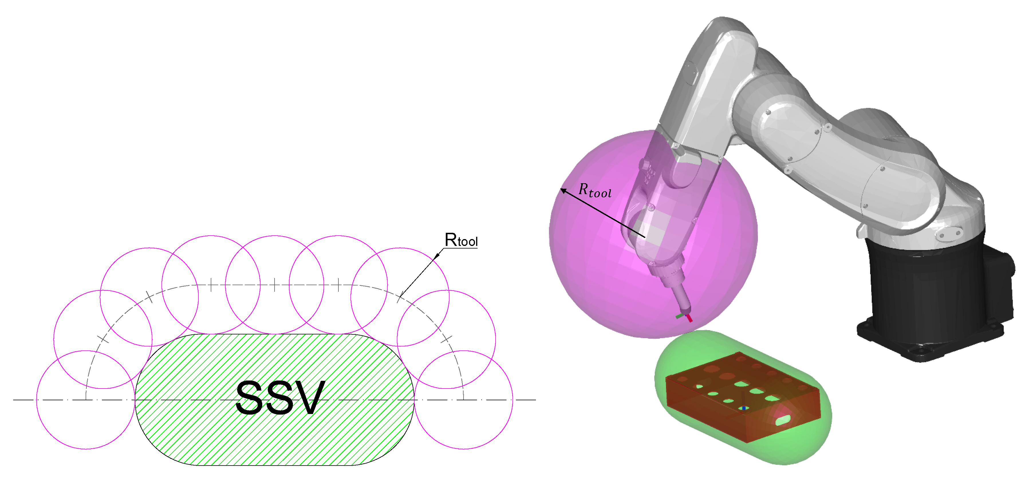
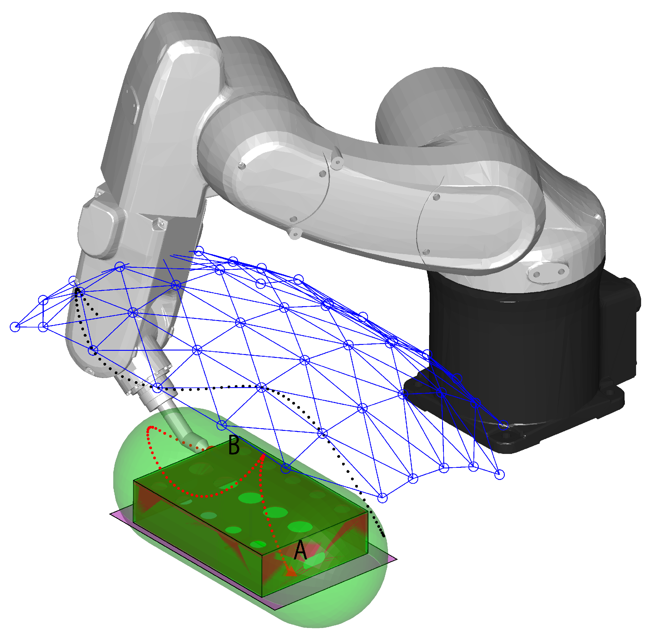
• Define a safe volume around the workpiece (the Swept Sphere Volume (SSV) shown in green in Figure 2);
  

  Figure 2. A simple scheme that shows the placement of the via points on a section of the Swept Sphere Volume (SSV) (to the left). Each section is then repeated many times around the symmetry axis of the SSV. All the via points are placed at a distance $R_{tool}$ from the surface of the SSV, so regardless the orientation of the wrist, the end effector will not collide with the work piece (to the right).
• Create a cloud of via points for the wrist center around the safe volume (Section 4.1), whose distance from the safe volume is equal to the distance between the tool tip and wrist center; such points are safe in the sense that, if the wrist center lies in one of the points, the tool cannot collide with the workpiece for any Joint 4, 5, and 6 values;
• Check if the via points are reachable by the robot from a kinematic point of view: if a collision occurs between the robot and the environment at some via points, they are removed from the cloud;
• Connect the via points to the eight closest ones (in the Cartesian space) to form the branches that will be used in the search of the minimum time path;
• Check the connections between the via points: if a collision occurs along the point to point motion between two connected via points, the connection is removed;
• Choose the initial ${\theta }_7$ values for starting and ending positions A and B (${\theta }_{7,A}$ and ${\theta }_{7,B}$);
• Find the suboptimal path that connects A and B without a collision using the Dijkstra algorithm to solve the graph whose nodes are the connected via points;
• Change ${\theta }_{7,A}$ and ${\theta }_{7,B}$ within a fixed grid around the initial values and loop from Point 8 until all possible combinations are evaluated;
• Find the combination ${\theta }_{7,A,opt}$ and ${\theta }_{7,B,opt}$ that yields the minimum time motion between A and B on the chosen grid.

The points from 8 to 10 can be iterated by refining the grid around the final point, until a certain condition is met (e.g., a maximum number of iterations). At the end of the iterations, the final values of redundant joint angles (${\theta }_{7,A,opt}$ and ${\theta }_{7,B,opt}$) are stored, and the corresponding graph is considered as the optimal path that connects A and B.

4.1. Via Points’ Generation and Selection

A line Swept Sphere Volume (SSV) [16] is used to encapsulate the workpiece. The shape and orientation of the SSV are chosen in a way that minimizes its volume.

Since the configuration of the tool is unknown a priori, to be sure that the tool does not collide with the workpiece, we chose to place the wrist of the robot at a distance greater than $R_{tool}$ from the SSV, where $R_{tool}$ is the minimum radius of a sphere centered in the wrist center and containing the tool. By using this criterion, a net of wrist center points equally distributed is placed on a surface at a distance of $R_{tool}$ from the SSV (Figure 2).

To create the point could, a section of the SSV, containing the SSV symmetry axis, is considered (Figure 2 on the left). On this plane, $m_1$ points are evenly placed at a distance $R_{tool}$ from the border of the SSV. Then, the section is cloned $m_2$ times around the SSV symmetry axis. The first and last points on each section that lie on the symmetry axis are considered once, so the total number of points is:

$$N_p=m_2(m_1-2)+2$$

(1)

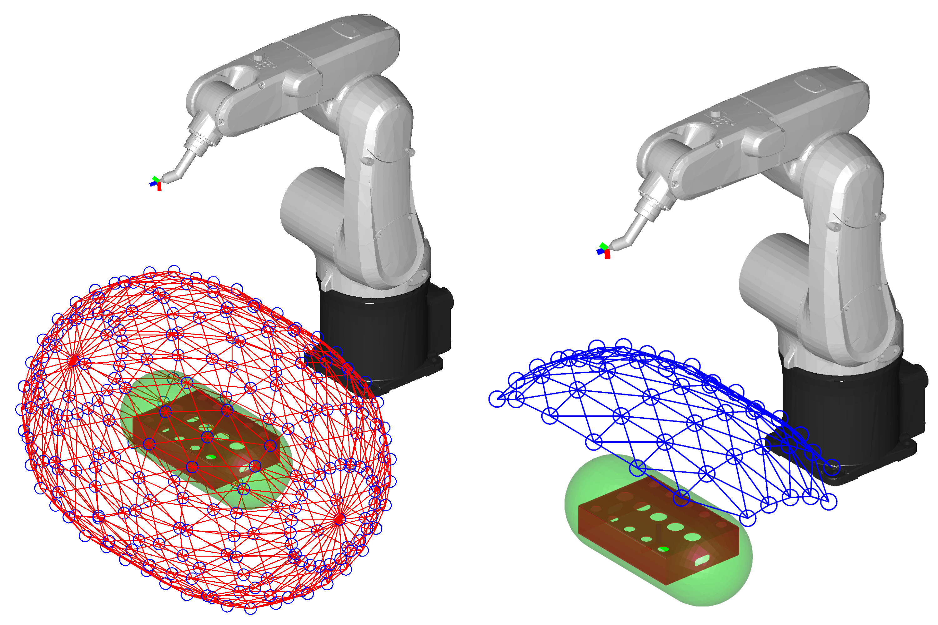
The density of the net is a design choice ($m_1$ and $m_2$) and has a direct effect on the performance of the Dijkstra algorithm [10]. Each point of the net is connected to its eight neighbors as shown in Figure 3, similarly to the uniform space sampling method shown in [29].

Figure 3. All the adjacent via points are connected to form the branches (to the left), and then, the unreachable via points and the branches that provide a collision are removed (to the right).

The first benefit provided by the proposed definition of via points is that, when the wrist center is in such points, the robot is in a safe position regardless of the orientation of the tool. In this way, if we include one of the via points in a motion between the starting and the ending points, such a via point will be safe for any configuration of the redundant axis in the given points. Thus, by creating a path that includes the given points and a subset of the calculated via points, such a path will be safe in all intermediate points for any choice of the initial and final configurations.

Secondly, since the via points are wrist center points, the inverse kinematic problem can be solved for the first three joints only (which is faster than solving the full problem), and an estimation of the motion time between connected points can be done by considering only such joints (Section 4.2, Equation (2)), thus drastically reducing the computational time. In fact, the estimated motion time on a given path depends only on the points chosen, regardless of the initial, pass-through, and final orientations of the tool. In this way, the time needed to move between different initial and final configurations of the robot can be evaluated without the need for re-calculating the inverse kinematics in the via points every time. To test the reduction of the computational time due to the decoupling of the inverse kinematic problem, a simple test was performed: the same position was used to calculate the entire configuration of the robot and only the first three joint values 100,000 times. The overall computational time for the whole inverse kinematic problem was 1.66 s, whilst the computational time required for the calculation of the first three joints was 1.06 s. As a result, the decoupling led to a reduction of the computational time of the inverse kinematic problem of around 36%.

Via points are checked for collision between the robot and the workpiece and the environment. If a collision is detected, the corresponding via point is deleted from the list. The collision test was performed as described in our previous work [3]: all the links were encapsulated inside SSVs, whilst all other objects were encapsulated inside Oriented Bounding Boxes (OBB [11]). In this way, it was possible to compute the interaction between the robot and the environment faster than with the usage of SSVs only [8].

4.2. Graph

The suboptimal path between two positions A and B is created using the Dijkstra algorithm [5]. To solve the algorithm, the branches and the nodes must be defined.

While the via points represent the nodes, the branches are represented by the connections between the via points. Considering the net of reachable via points, only adjacent via points (in Cartesian space) are connected to form branches (Figure 3 on the left), so that the total number of branches is reduced. To avoid unnecessary calculations, collision tests along the motions through all the branches are computed. If a collision is detected, the corresponding branch is removed (Figure 3 on the right).

Branches’ weight equal the robot movement time between the nodes. Movement time between nodes h and k is estimated considering only the first three joints:

$$T_{hk}=\underset{j=1,2,3}{max}\left\{\frac{|\Delta q_{j,hk}|}{{\dot{q}}_{max,j}}{c}_v\right\}$$

(2)

where $\Delta q_{j,hk}$ is the total rotation of joint j between the nodes h and k, ${\dot{q}}_{max,j}$ is the maximum speed of joint j, and $c_v$ is the velocity coefficient of the motion law [2].

Starting and ending nodes are defined by points A and B; A and B are connected to all the via points to form additional branches. In this way, it is possible to enter (from A ) and exit (towards B) the cloud of via points from any one of the via points. The weights of the additional branches are calculated as the traveling times (as Equation (2)), and the connections are checked to find collisions: the branches that provide collision are removed. The Dijkstra algorithm calculates the graph using A as the first node and B as the last one.

The first ${\theta }_{7,A}$ and ${\theta }_{7,B}$ values are null to start the optimization algorithm around the position provided by the user. To find the optimal solution, the redundant joint angles ${\theta }_7$ at A and B are changed by fixed steps ($\delta \theta$), from minimum values (${\theta }_{7,i,min}$) to maximum ones (${\theta }_{7,i,max}$). In this way, a fixed grid of possible combinations is created; the limits of the grid can be different for A and B (see Table 1 for an example).

Table 1. An example of iterations changing $\delta \theta$ from ${60}^{\circ }$ to $1^{\circ }$. Such values were used to run the algorithm in Test 1.

Step	$\mathit{\delta }\mathit{\theta }$	A Bounds (${}^{\circ }$)	B Bounds (${}^{\circ }$)	${\mathit{\theta }}_{7,\mathit{A},\mathit{opt}}$	${\mathit{\theta }}_{7,\mathit{B},\mathit{opt}}$
	(${}^{\circ }$)	(${\mathit{\theta }}_{7,\mathit{A},\mathit{min}}$,${\mathit{\theta }}_{7,\mathit{A},\mathit{max}}$)	(${\mathit{\theta }}_{7,\mathit{B},\mathit{min}}$,${\mathit{\theta }}_{7,\mathit{A},\mathit{max}}$)	(${}^{\circ }$)	(${}^{\circ }$)
1	60	[−180, 180]	[−180, 180]	0	60
2	45	[−135, 135]	[−75, 195]	0	60
3	30	[−120, 120]	[−60, 180]	0	30
4	20	[−80, 80]	[−50, 110]	0	10
5	10	[−40, 40]	[−30, 50]	−10	20
6	5	[−30, 10]	[0, 40]	−15	20
7	2	[−23, −7]	[12, 28]	−15	22
8	1	[−19, −11]	[18, 26]	−14	23

To ensure that the calculated paths are feasible, a collision test along each suboptimal path is computed. To do so, the planning of robot motion is performed along the whole path, including wrist rotations. The angles of the first three joints are interpolated from A values to B values considering also the via points included in the path. The angles of the last three joints, on the other hand, are interpolated from A values to B values only, since their values are not assigned at the via points. If a collision is found, the graph is re-calculated. This may occur due to a possible colliding configuration of the robot provided by the values of Joints 4, 5, and 6 along one of the connections; in fact, wrist rotations have not been considered in the previous collision tests, and whilst the via points are safe regardless of wrist orientation, connecting paths (especially from A to the cloud and from the cloud to B) may not.

The final movement time of the path is given by the following expression:

$$T_{final}({\theta }_{7,A},{\theta }_{7,B})=max\left\{T_{Dijkstra}({\theta }_{7,A},{\theta }_{7,B}),\underset{j=4,5,6}{max}\left\{\frac{|\Delta q_{j,AB}({\theta }_{7,A},{\theta }_{7,B})|}{{\dot{q}}_{max,j}}{c}_v\right\}\right\}$$

(3)

where $T_{Dijkstra}({\theta }_{7,A},{\theta }_{7,B})$ is the minimum time yielded by the Dijkstra algorithm and $\Delta q_{j,AB}({\theta }_{7,A},{\theta }_{7,B})$ is the total rotation of joint j between points A and B.

At the end of an iteration step, all the possible combinations of ${\theta }_{7,A}$ and ${\theta }_{7,B}$ are compared. The best combination of those two values, i.e., the one that minimizes $T_{final}$, provides ${\theta }_{7,A,opt}$ and ${\theta }_{7,B,opt}$ that are to be used in the next iteration step. To start the next iteration step, the value of $\delta \theta$ is reduced and the next boundaries of ${\theta }_{7,A}$ and ${\theta }_{7,B}$ are changed. The lower $\delta \theta$, the better the precision of the optimal position. In the first iteration, ${\theta }_{7,A,min}={\theta }_{7,B,min}=-{180}^{\circ }$ and ${\theta }_{7,A,max}={\theta }_{7,B,max}={180}^{\circ }$ to evaluate the entire workspace (Table 2).

Table 2. Values of ${\theta }_{7,A}$ and ${\theta }_{7,B}$ when the first iteration step has $\delta \theta ={60}^{\circ }$.

$\mathit{\delta }\mathit{\theta }$(${}^{\circ }$)	60
${\mathit{\theta }}_{7,\mathit{A}}$ values (${}^{\circ }$)	[−180, −120, −60, 0, 60, 120, 180]
${\mathit{\theta }}_{7,\mathit{B}}$ values (${}^{\circ }$)	[−180, −120, −60, 0, 60, 120, 180]
Number of combinations	49

At the end of the procedure, the optimal couple of redundant joint angles ${\theta }_{7,A,opt}$ and ${\theta }_{7,B,opt}$ is provided.

The optimal solutions are not to be intended as the globally optimal solutions to the problem. Since this is a nonlinear stochastic problem that has to face many constraints (collision avoidance, movement between the via points, discretization of the values of the redundant joint angle), the purpose of the algorithm is to find a local minima of the problem, which, however, can be good enough to satisfy the majority of the industrial scenarios.

5. Validation

A MATLAB^® script was created through which an ADEPT VIPER s650 six axis robot was simulated (Figure 2) moving from one working position to another. The PC used for the simulation was powered by an Intel Core i7-2700K, 16 GB of RAM, and 64 bit Windows 10 Pro 1803 version.

The robot was moved from one side of the workpiece to another so that direct movement was impossible (the robot would collide with the workpiece). The collision check along the movement was performed at a frequency of 180 Hz.

The starting position was $P_A$ (490, 167.5, 18.4) with the orientation defined by Cardan angles $\{x,y,z\}=\{0,90,-90\}$. The ending position was $P_B$ (410, −67.5, 48.4) with the orientation defined by Cardan angles $\{x,y,z\}=\{0,90,90\}$. The robot base frame was coincident with the global reference frame. The parameters of the planes defining the workpiece’s OBB, used by the collision detection algorithm, are shown in Table 3. Moreover, another plane was added to simulate the table where the workpiece was placed. The parameters describing this plane are in the seventh column of Table 3.

Table 3. Parameters describing the 6 planes that define workpiece Oriented Bounding Box (OBB) (Columns 1–6) and the extra plane describing the table where the workpiece is placed (Column 7). The parameters refer to the point normal form of the equation of a plane: $ax+by+cz+\lambda =0$.

Plane ${\mathit{n}}^{\circ }$	1	2	3	4	5	6	7
a	1	−1	0	0	0	0	0
b	0	0	1	−1	0	0	0
c	0	0	0	0	1	−1	−1
$\lambda$ (mm)	−368	532	67	167	1.6	55.4	1.6

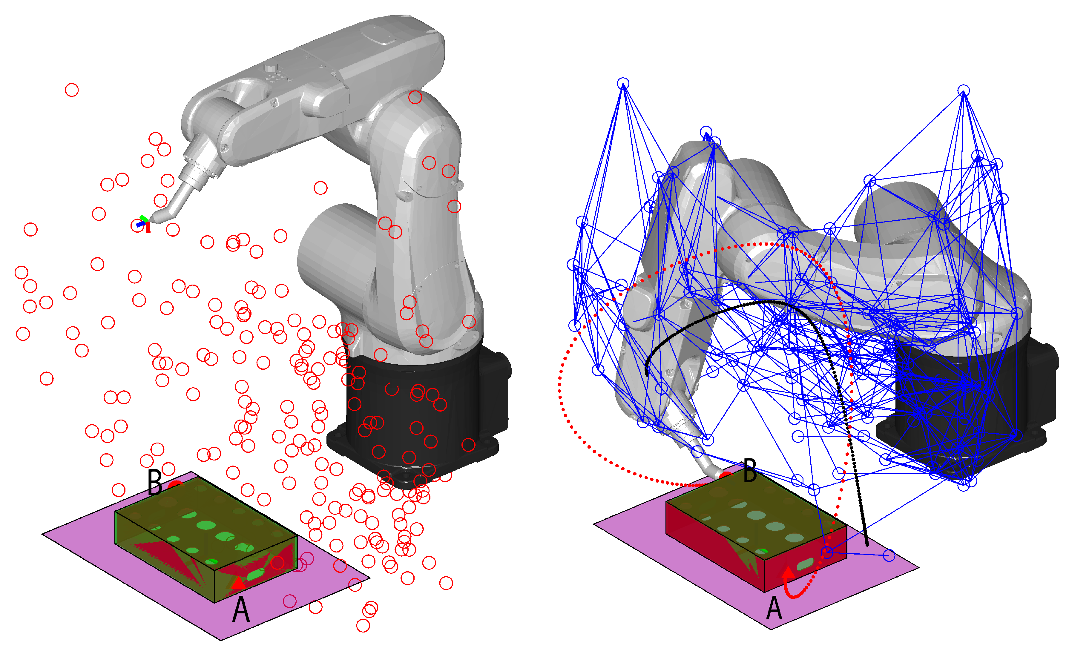
The total net of via points was made of 227 points ($m_1=11$, $m_2=25$), while the number of feasible via points was 56, and the number of via points connected to the graph was 46 (Figure 3 to the right).

In this test, we set the range limits of ${\theta }_7$ angles to $\pm 3$ times $\delta \theta$ (first two steps) and $\pm 4$ times $\delta \theta$ (for other steps, see Table 1). This ensured a good trade-off between algorithm performance and computational time, since for each iteration, it limited the number of computations of the graph.

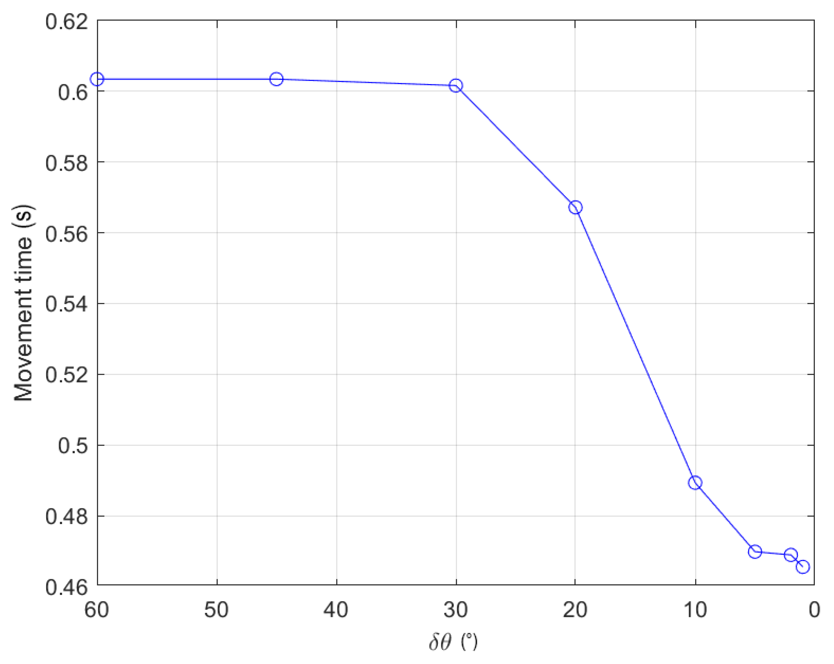
At first, the lowest movement time at each iteration step was evaluated. In Figure 4 are shown the results: the lowest movement time decreased from the highest $\delta \theta$ (${60}^{\circ }$) to the lowest one ($1^{\circ }$). In this case, the reduction of the movement time from the higher value of $\delta \theta$ to the lowest one was nearly $23\%$ (Table 4). The computer took 24.88 s to find out ${\theta }_{7,A,opt}$ and ${\theta }_{7,B,opt}$ with eight steps. The best combinations at each step can be seen in Table 1.

Figure 4. Minimum of moving total time for each step value. The x-axis direction has been reversed to show the iteration process from left to right.

Table 4. Results of the test changing $\delta \theta$ from ${60}^{\circ }$ to $1^{\circ }$.

Step	$\mathit{\delta }\mathit{\theta }$	Lowest Movement Time (s)	Comparison to Step 1 (%)	Total Computational Time (s)
1	60	0.6035	100	1.77
2	45	0.6035	100	3.47
3	30	0.6016	99.7	6.54
4	20	0.5672	94.0	10.42
5	10	0.4893	81.1	14.35
6	5	0.4698	77.8	17.89
7	2	0.4689	77.7	21.37
8	1	0.4655	77.1	24.88

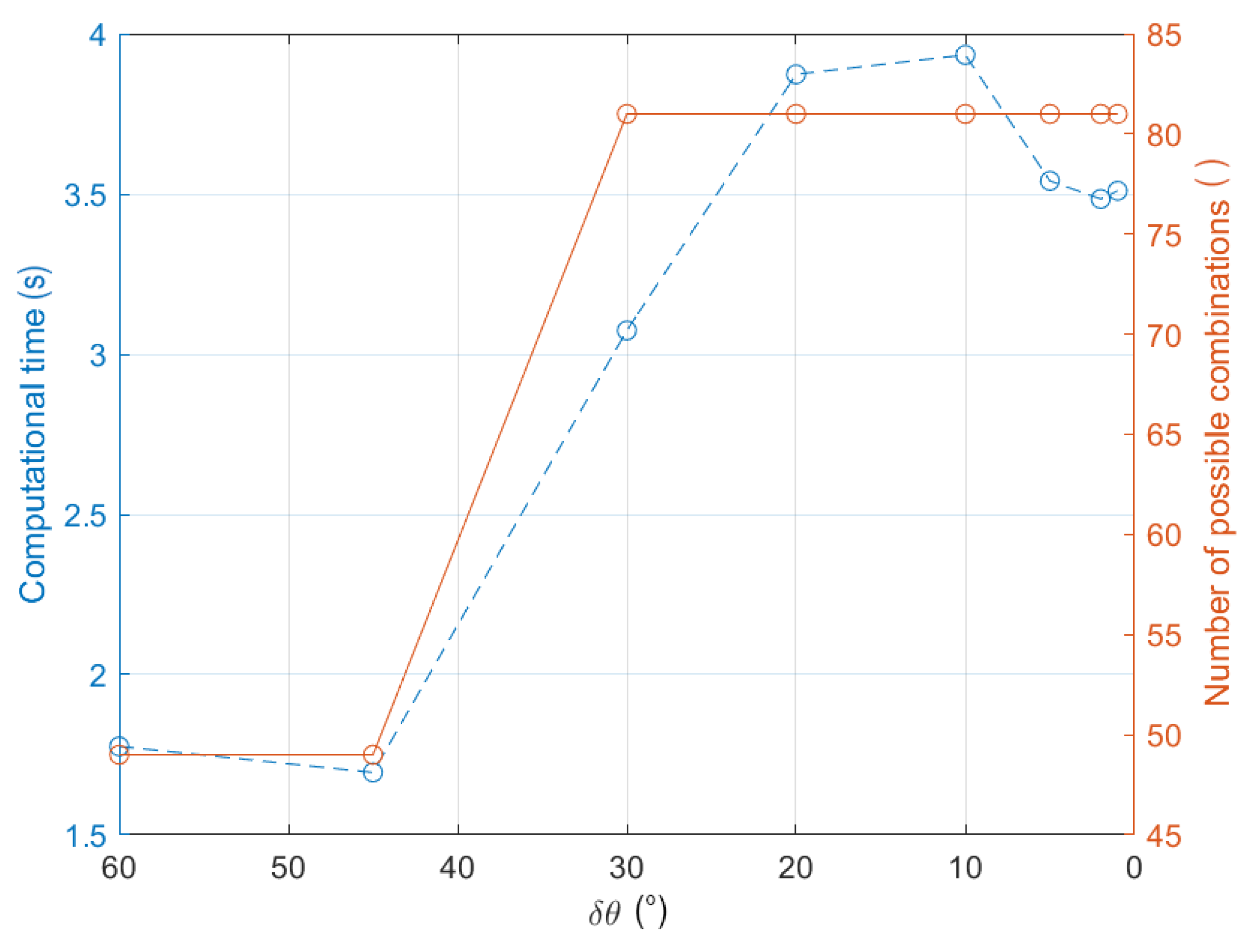
Figure 5 shows the calculation times and the number of possible combinations of each $\delta \theta$ step. The calculation times nearly followed the trend of the number of combinations and was capped to the maximum of 81 starting from the third step. Then, at small $\delta \theta$ values, the calculation times slightly dropped due to a smaller amount of colliding paths: small variations of ${\theta }_{7,A}$ and ${\theta }_{7,B}$ around the optimal solution usually did not lead to many path collisions.

Figure 5. Computational time of the definition of the graph for each step value. The computational time nearly follows the number of possible combinations. The x-axis direction has been reversed to show the iteration process from left to right.

Even if a single calculation of 24.88 s reduced the movement time of nearly $23\%$, a similar result can be obtained using a reduced number of steps. We performed another test with the same starting and ending positions, but with only two iteration steps: $\delta {\theta }_1={30}^{\circ }$ and $\delta {\theta }_2=5^{\circ }$. The results (Table 5) showed that with reduced computational times (only $11.41$ s), the lowest movement time was nearly the same as in the previous test.

Table 5. Results of the test changing $\delta \theta$ from ${30}^{\circ }$ to $5^{\circ }$.

Step	$\mathit{\delta }\mathit{\theta }$	Lowest Movement Time (s)	Comparison to Step 1 (%)	Total Computational Time (s)
1	30	0.6016	100	5.05
2	5	0.4698	78.1	11.41

In Figure 6, the final movement provided by the algorithm with the parameters of Table 5 is shown. The shape of the path depended on the density of the via points defined in the workspace.

Figure 6. From the top: the final movement provided by the algorithm for Test 1, with the red dots that describe the end effector trajectory and the black dots that describe the wrist center trajectory. To the bottom: corresponding joint angles versus time.

Comparison with PRM

A comparison of the proposed method with the Probabilistic Roadmap Method (PRM) was performed, to compare the solutions obtained and the computational times. The PRM is a sampling based method that uses the Dijkstra algorithm to connect two points defined in the configuration space by using randomly generated via points defined in the configuration space. The main differences with our method are that: (a) the via points were defined randomly (i.e., without considering workpiece actual encumbrance); (b) wrist rotations were assigned at the via points, and this would force the wrist joints to make wider rotations along the path with respect to our method.

In the comparison, the PRM was set as follows:

• The sampling of the configuration space of the robot was performed by randomly choosing 227 configurations (equal to the number of via points of our point cloud);
• The configuration space was searched within a limited range of Joint 1, 2, and 3 rotations to reduce the dispersion of the randomly generated points (which would result in worse performance of the PRM algorithm); Joint 4, 5, and 6 ranges were not limited, to avoid loosing dexterity;
• Each configuration was connected to the nearest eight configurations (in the configuration space).

With the aim of fitting the PRM to the method described in Section 4, the latter was modified as follows:

• Point b was eliminated;
• Point c was modified since the via points were provided by randomly generated samples in the six-dimensional configuration space;
• Point e was modified since the via points were connected to form branches by finding the eight closest points in the configuration space.

All the other points of the method were kept unchanged.

Since in the PRM the via points were randomly generated and may yield variable results, 400 instances of the PRM were performed (with two $\delta \theta$ steps as in Table 5). The simulations showed a mean computational time of 21.2 s (standard deviation of 3.38 s) and a mean robot movement time of 0.6915 s (standard deviation of 0.2177 s). An example of the PRM solution is shown in Figure 7, where among 227 random samples, only 133 via points were reachable and connected to the graph. In this particular case, both the computational time and mean movement times were greater than with our method.

Figure 7. The wrist center points provided by Probabilistic Roadmaps (PRM) (to the left) and the corresponding final movement provided for Test 1, with the red dots that describe the end effector trajectory and the black dots that describe the wrist center trajectory (to the right). Blue circles are feasible and connected wrist center points.

This was due to the sparse location of the via points in the PRM, most of which were not useful in the definition of a path with a low movement time. Moreover, the search for the suboptimal path was performed within a six-dimensional space in the PRM (the configuration space), while the decoupling of the inverse kinematic problem in our approach allowed searching a three-dimensional space and then simply interpolating the start and end values of the last three joints, thus reducing the computational effort [22].

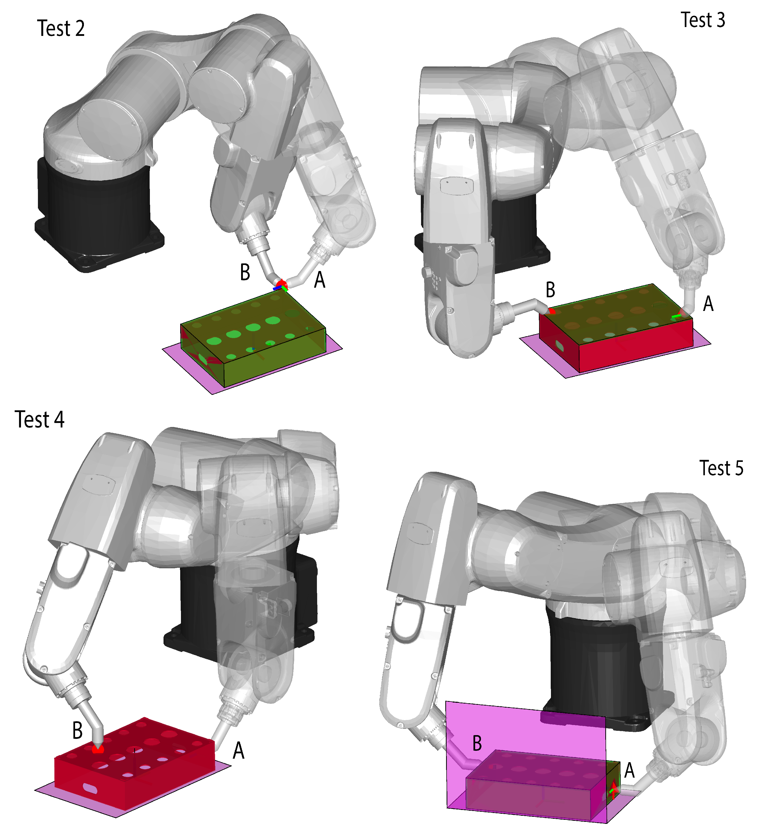
To better understand the difference between our method and the PRM, five different cases were considered, in which the starting/ending positions and/or the workcell layout were changed (Figure 8): Test 1 was the same as in Figure 6; Test 2 and Test 3 were very simple movements (Test 2 was a simple rotation around end effector position; Test 3 was a tool repositioning on the same surface on top of the work piece); Test 4 included a tool repositioning from one side to the top of the workpiece; Test 5 included the same movement of Test 1 with an additional obstacle to constrain the movement.

Figure 8. Starting (A) and ending (B) robot configurations of Tests 2 to 5; redundant angles are null in all the positions depicted (${\theta }_{7,A}=0$ and ${\theta }_{7,B}=0$).

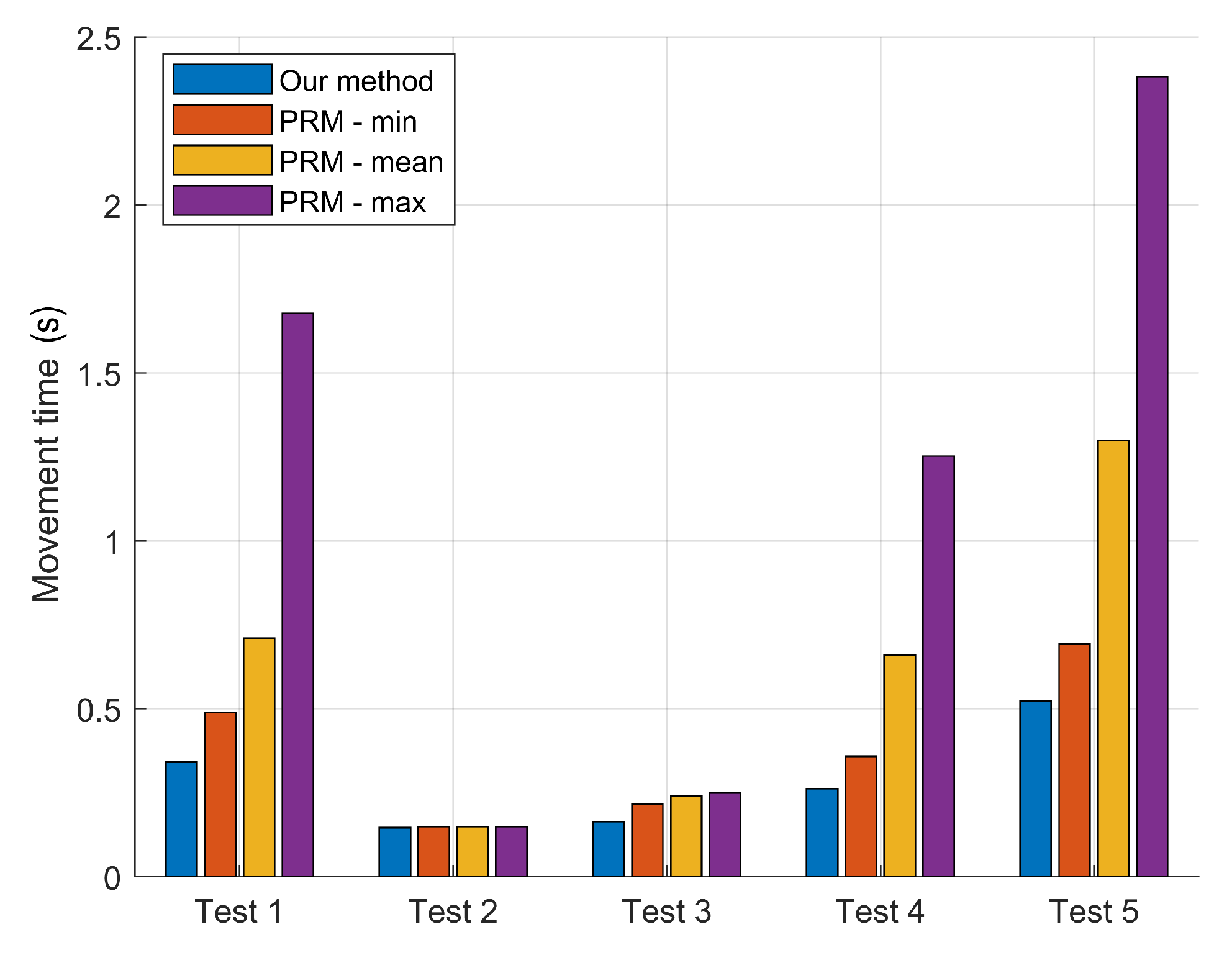
Figure 9 shows optimal movement times provided by our method and by the PRM in the five tests (for the PRM, which was repeated 10 times for each test, minimum/maximum and mean values are depicted). Except from Test 2 (simple tool repositioning), where the results were comparable, our method outperformed the PRM in terms of the minimization of robot movement time. It may be that the PRM would perform better if we increased the number of the generated via points; however, this would dramatically increase computational time.

Figure 9. Optimized movement times retrieved from our method and from PRM. Since PRM planning was repeated 10 times for each test, the chart shows the minimum, mean, and maximum optimal times from PRM for each test.

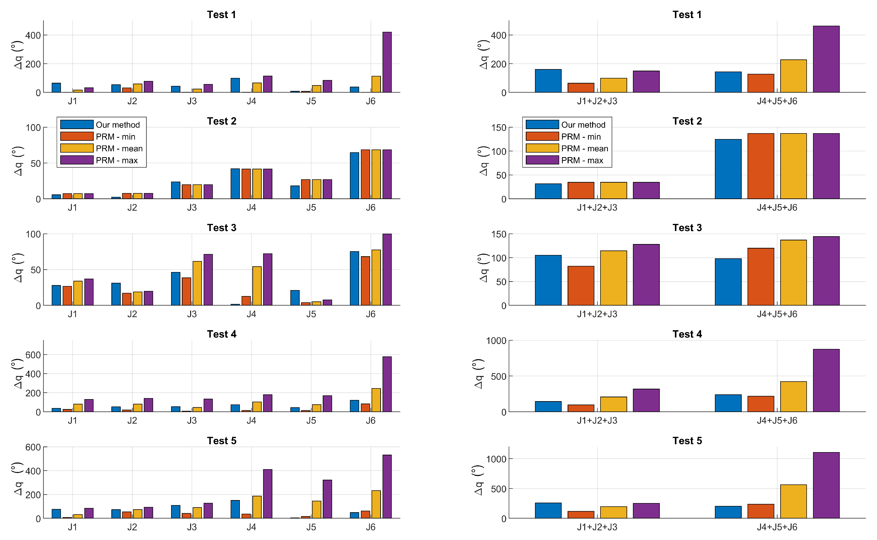
Figure 10 shows the total absolute joint displacements along the optimal path provided by our method and by the PRM in the five tests (for the PRM, which was repeated 10 times for each test, minimum/maximum and mean values are depicted). Cumulative displacement of the first three joints, which accounted for wrist center motion, and of the last three joints, which accounted for wrist rotation, are shown as well. This figure provides a possible explanation of the results shown in Figure 9: the PRM tended to produce wider displacements of the last three joints (i.e., wider rotations of the wrist), since it assigned their values in the via points; as a result, the motion time increased with respect to our method, where the displacement of the wrist joints was minimized (it equaled the difference between initial and final rotations in A and B). Even though our method may have sometimes provided wider rotations of the first three joints (i.e., larger motion of the wrist center), this seemed not to be the bottleneck in the tests performed.

Figure 10. Joint displacement for each joint for each test (to the left) and the corresponding sum of joint triplets (to the right). Since PRM planning was repeated 10 times for each test, the chart shows the minimum, mean, and maximum displacements from PRM for each test.

Another interesting point is that, since the PRM is a stochastic method (in the sense that it produces a random set of via points), a single execution of it may yield very bad results in terms of robot movement time. On the other hand, our method provided a very good solution in one single shot.

6. Conclusions

In this paper, we dealt with the problem of defining a trajectory of an industrial robot from a given position to another, when the task is redundant around the tool axis. We proposed a new optimization technique, which finds the initial and final angles of the redundant axis and a proper sequence of via points that minimizes the movement time between the given positions while avoiding collisions with the obstacles at the same time.

The presented method was based on the automatic generation of a cloud of Cartesian via points around the workpiece for the wrist center, thus decoupling the inverse kinematic problem. The method used the Dijkstra algorithm to find the suboptimal path that connected the start and end positions passing through the via point cloud, and a final check for collision was performed to validate the solution. The algorithm can iteratively evaluate a high number of starting and ending configurations in low computational time, allowing one to perform a reasonably wide search of the suboptimal path within the infinite possible motions between the given points.

The particular choice of the via points in our algorithm allowed not only reducing the computational time, but also and mainly minimizing wrist rotations along the path, which in turn helped to obtain low robot motion times. A direct comparison of our method to the PRM in the case of an anthropomorphic industrial robot showed, in four out of five tested motion tasks, that our method could outperform the PRM in terms of robot optimal motion time, at a lower computational cost. Such results should be validated in a wider number of cases; however, their interpretation provided by the analysis on joint rotations suggested that they may be generalized.