1. Introduction
Single-Actuator Mobile Robots (SAMR) are robots with the ability to explore environments with relatively high freedom using only one motor. The most direct consequences and advantages of using a single actuator are savings in costs, energy consumption, size, and weight. Due to these advantages, SAMR robots are especially appropriate for applications that require energy autonomy, miniaturization, and navigation in difficult-to-access areas, with the purpose of performing inspection, cleaning, reconnaissance or search-and-rescue tasks, among others [
1].
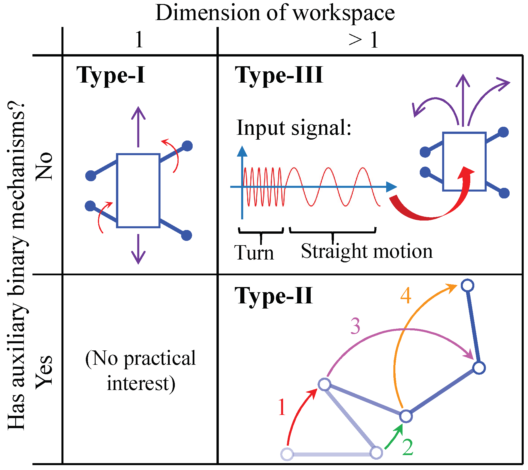
Most SAMR robots reported in the specialized literature can be classified into one of three main types (type-I, type-II, or type-III), depending on two criteria: the dimension of their workspace, and the existence of auxiliary binary mechanisms that help the robot to change the direction of motion. This classification, which we propose in this paper, is illustrated in
Figure 1.
Type-I SAMR are robots that use a single actuator to control their motion along a one-dimensional workspace, with no additional mechanisms. For example, the authors in [
2] presents an octopod that can walk forward or backwards along a straight line by means of a single motor and a system of cams that synchronize the motion of all its eight legs. Similarly, the authors in [
3,
4] present two climbing robots that can vertically climb using a single actuator each. Another single-actuator climbing robot is presented in [
5]; this robot swings a pendulum to dynamically climb the vertical space between two walls by bouncing between these walls. The authors in [
6] present a robot that can climb or move along a straight line by using a wave-like locomotion generated by a single motor. Type-I SAMR robots can only move along one dimension. In order for these robots to be able to change the direction of their motion and control their motion in higher-dimensional workspaces (e.g., plane or space), it would be necessary to equip them with additional motors [
4,
6], and thus they would no longer be single-actuator mobile robots.
According to
Figure 1, type-II SAMR have workspaces with dimensions higher than one, i.e., they are not constrained to move along a straight line only, but they can typically control their position and orientation in a plane. In addition to having a main continuous actuator, type-II SAMR are characterized by having also some additional binary mechanisms that allow the robot to modify its topology, changing in this way the effect that its single main actuator exerts on the overall motion of the robot. In other words: strictly speaking, type-II SAMR robots should be called “Single-Actuator Mobile Robots...
with auxiliary binary actuators” (nevertheless, some authors of these robots regard them as single-actuated). Thanks to these auxiliary binary actuators, the driving force generated by the only continuous actuator of the robot can be channeled as required, e.g., to produce straight motion, to change the direction of motion, to jump, etc. Note that these auxiliary binary actuators do not necessarily need to be motors or actuators in the usual sense of the term, but they can simply be electromagnets, suction cups, or clutches that engage or disengage two mobile parts of some internal mechanism of the robot, in order to transmit the driving force of the only continuous actuator to different mechanisms and modify the overall motion of the mobile robot.
Some examples of type-II SAMR robots can be found in the literature. For example, the authors in [
7] present a mobile robot with two variable-radius wheels driven by a single motor such that, when activating a clutch, this motor also displaces the center of mass of the robot along its main shaft, which modifies the relative radii of the wheels and produces a change in the direction of motion due to differential drive kinematics. The authors in [
8,
9] propose snake-like robots powered by a single tendon-driven actuator each robot. These robots are made up of several segments rigidly connected by welded joints such that, when applying an electric current to some of these welds, can temporarily melt them in order to modify the geometry of the robots. By selectively melting these welded joints and actuating their only motor, these robots can move along straight lines, change their direction in a plane, or perform out-of-plane motions. Finally, the authors in [
10] present the DynaRoACH robot, which is inspired by cockroaches and has a single actuator to move along straight lines. This robot can also turn by modifying the relative stiffness of its legs through shape-memory alloys. Similarly, the DASH robot [
11] is a single-motor hexapod that can steer or walk straight by respectively introducing or removing small asymmetries between its legs, by means of shape-memory alloys.
Type-III SAMR typically are under-actuated mobile robots that use a single actuator and lack auxiliary binary mechanisms, and they are able to control their motion in more than one dimension. Usually, these robots will perform some type of motion or other (e.g., moving along a straight line, turning, jumping...) depending on the characteristics (amplitude, sign, frequency...) of the input signal applied to its only actuator. For example: [
12] presents a robot that swims over water surfaces, this robot is driven by a single actuator that produces straight motion when excited at constant frequency, whereas it modifies the direction of motion when being excited at different frequencies during each semi-period. The authors in [
13] develop a micro-robot made up of a single piezoelectric actuator that makes the robot move in straight lines or turn left/right depending on the natural frequency at which this actuator is excited. A similar cubic robot is presented in [
14], where the robot can move straight or turn by exciting its only actuator (a dielectric elastomer resonator) at different resonant frequencies. Zuliani et al. [
15] developed an origami hand that can adopt different configurations (with different fingers extended or folded) depending on the excitation frequency of its only actuator. Although this is not a mobile robot, the idea might be exploited to build small and lightweight single-actuated legged origami robots. In [
16], a spherical robot is proposed, which is able to either move straight or steer by rotating its only internal motor at constant or alternating velocity, respectively. The authors in [
1] present a single-actuated hexapod robot whose legs have different stiffnesses; this robot will walk in straight lines or turn left/right depending on the shape of the velocity profile introduced to its only motor. Ribas et al. [
17] designed a single-motor tricycle robot that can steer and move forward describing undulatory trajectories by pivoting alternatively about each of the rear wheels, similar to our robot proposed in the present paper. The front wheel of this tricycle can freely steer, displacing the instantaneous center of rotation from one rear wheel to the other by inverting the spin of the motor. In [
18], a robot consisting of a single large wheel with only one motor is presented: if this motor oscillates between two limit positions, the robot rolls along a straight line. If the motor overcomes one of such limits, then a spring is compressed and its elastic energy is suddenly released, which produces the jump of the robot to overcome steps and other obstacles. Finally, the authors in [
19,
20] present jumper robots that can perform different movements using only one motor: jumping (by compressing springs), standing up after the jump, modifying the direction of the next jump, or panning a camera mounted on the robot. These robots will perform some or other motions depending on the amplitude and sign of the rotation of their only motors.
Comparing the three types of SAMR robots identified, generally one of the main drawbacks of type-III SAMR is that it may be difficult to precisely control their motion [
1], since it largely depends on their under-actuated dynamics. On the contrary, it is relatively easy to precisely control the motion of type-II SAMR robots by using their auxiliary binary actuators. Type-I robots are usually simpler but they can only move along one dimension. Note that the bottom-left cell in the classification table of
Figure 1 is empty because it would not have much practical interest to design SAMR robots that have auxiliary binary mechanisms but can only move along one-dimensional workspaces (the purpose of these binary mechanisms is precisely to increase the dimension of the workspace).
Acknowledging the higher simplicity and flexibility of type-II SAMR robots, this paper presents the MASAR: a new
Modular
And
Single-
Actuator
Robot that explores two-dimensional environments by rotating about binary pivots that are alternately adhered to the environment or detached as required, as illustrated schematically in the bottom-right cell of
Figure 1. Contrary to previous type-II SAMR, the proposed robot is capable of performing concave transitions between orthogonal planes, which makes it especially suitable for exploring indoor environments delimited by floors, walls, and ceilings. In addition, the proposed robot can combine with other identical modules in order to form more complex modular reconfigurable robots. This paper focuses on the trajectory analysis of the proposed robot, in order to follow polygonal paths composed of chains of straight segments that may include narrow sections that constrain the movements of the robot.
This paper is organized as follows. First,
Section 2 presents the proposed MASAR robot. Then,
Section 3 solves its path tracking problem in the case of polygonal paths with narrow sections that must be traversed. Next,
Section 4 illustrates the proposed path tracking solution with some examples and experiments that deepen into the problem. Finally,
Section 5 presents the conclusions and future work.
2. MASAR: A New Modular And Single-Actuator Robot
This section presents a new type-II SAMR robot, whose trajectory analysis is the main focus of the present paper. This robot is depicted in
Figure 2a, and it has been called MASAR, which is the acronym of “Modular And Single-Actuator Robot”. MASAR is patented with Ref. number ES2684377 and priority date 31 March 2017.
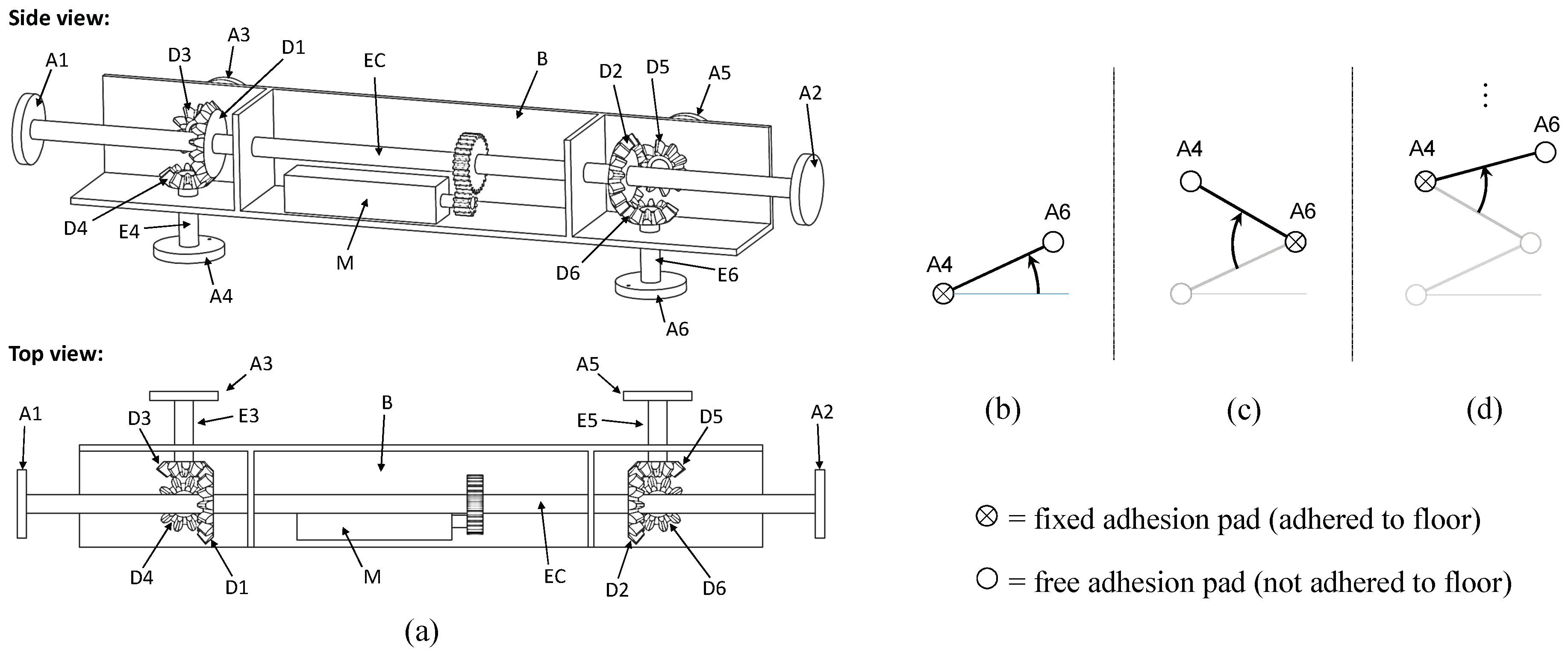
As illustrated in
Figure 2a, MASAR has a main body B rigidly attached to a single motor M that drives a central shaft EC that can rotate with respect to body B. At each side of the motor M, there is a mechanism comprised of three bevel gears with mutually orthogonal and intersecting axes: gears D1, D3, D4 to the left of M, and gears D2, D5, D6 to the right. Gears D3, D4, D5, D6 are connected to respective small shafts E3, E4, E5, E6 that can rotate with respect to the main body B; these axes have adhesion pads A3, A4, A5, A6 at their ends (see
Figure 2a). Likewise, the central shaft EC has adhesion pads A1, A2 at both ends.
According to the classification of
Figure 1, MASAR is a type-II SAMR robot because it has several binary adhesion pads (A1, A2, A3...), each of which may be ON or OFF (i.e., adhered to the environment or not adhered to it, respectively). The locomotion of this robot is as follows. Assume that the robot is initially resting on the floor through pads A4 and A6, as in the previous
Figure 2a. Assume also that only pad A4 is ON (i.e., adhered to the floor). When actuating motor M in this situation, since A4 is rigidly adhered to the floor, the central shaft EC (and the whole robot, as a consequence) will rotate about the axis of E4, since the bevel gear D1 will roll on gear D4, which is static because A4 is adhered to the floor. This motion is illustrated in
Figure 2b, which represents schematically a top view of the robot. After rotating the robot about E4, the adhesion pad A6 would be turned ON, whereas A4 would be turned OFF, and powering the motor in that case would produce the rotation of the whole robot about axis E6, as indicated in
Figure 2c. By alternately turning ON and OFF pads A4 and A6, the robot would walk on the floor describing some desired trajectory (see
Figure 2d or
Figure 1).
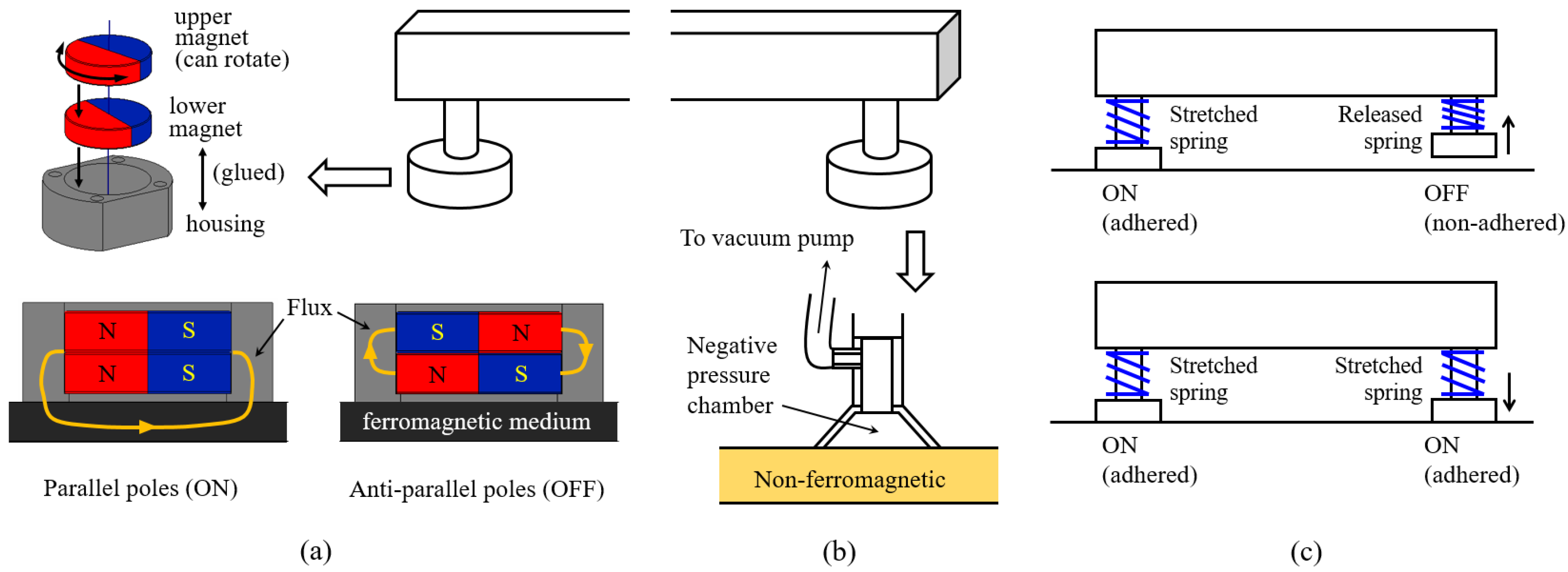
Regarding the adhesion pads, the technology to implement them should not be different from other adhesion technologies generally used in climbing robots. Of all adhesion technologies used in climbing robots [
21], magnetic and pneumatic technologies are the most mature and widely used ones, and these should be the adhesion technologies used for the adhesion pads of the MASAR robot. The choice to use one or another technology will depend on the medium on which the robot moves:
If the MASAR robot is used for exploring industrial infrastructures, made of ferromagnetic materials, then the best choice will be magnetic adhesion, preferably
switchable permanent magnets [
22]. As illustrated in
Figure 3a, switchable magnets are made of cylindrical and diametrically magnetized permanent magnets embedded inside a ferromagnetic housing such that, by rotating by 180°, one of the magnets with respect to the other using a micromotor, their magnetic poles remain parallel or anti-parallel, recirculating the magnetic flux either through the ferromagnetic medium (ON state: producing the adhesion to it) or internally through the housing (OFF state: canceling adhesion). Switchable magnets have many advantages over classical electromagnets [
23], such as lower energy consumption (power is only needed for switching the adhesion state, instead of continuously draining power to remain attached), higher adhesion forces per unit mass, and higher safety (in the event of power failure, permanent magnets will not detach). Examples of binary switchable magnets were developed in [
22] for a climbing biped robot.
If the environment where the MASAR robot moves is not ferromagnetic, such as domestic environments, then magnetic adhesion is not feasible and active pneumatic adhesion should be used instead. Active pneumatic adhesion requires using suction cups inside which a negative pressure is produced by means of a vacuum pump (
Figure 3b). Thus, in case pneumatic adhesion was required, each MASAR robot will have to carry a small vacuum pump in addition to a battery to power the pump and other elements of the robot, as in the robot presented in [
24].
Independently of the adhesion technology used for the adhesion pads, it is clear from
Figure 2 that the OFF adhesion pad will rub against the floor, which may hinder the motion of the robot in case the floor is not sufficiently smooth (e.g., pad A6 will rub when it rotates about pad A4 in
Figure 2b). If necessary, this can be overcome by introducing an additional translational articulation to each adhesion pad, such that each pad remains retracted when OFF (just the minimum distance necessary to prevent rubbing against the floor), but it is slightly extended when ON, to guarantee that it makes contact with the floor (see
Figure 3c). This may be implemented with electromagnets or other specifically designed mechanisms, which are commanded by the very same ON/OFF signal that activates or deactivates the adhesion of the pad to the environment. The concrete definition of this system is part of ongoing and future work, together with the development of a prototype of the proposed robot.
A similar robot that also uses the mode of locomotion shown in
Figure 2b–d was developed in [
25] for autonomous cleaning of glass windows. In [
25], two opposite pads similar to our pads A4 and A6 are simultaneously powered by the same motor by means of a belt mechanism with parallel axes, whereas our robot uses the bevel-gear mechanisms with concurrent axes depicted in
Figure 2a. In addition to this difference, our robot also has two additional differences with respect to the one described in [
25]:
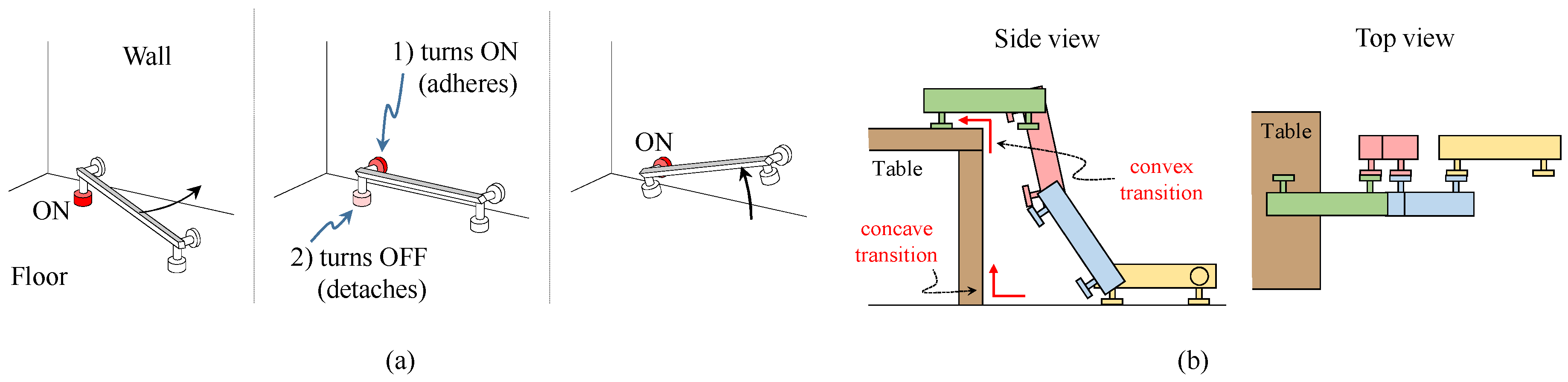
MASAR can perform concave plane transitions, such as those necessary for traversing between a vertical wall and the floor/ceiling or between different walls (see
Figure 4a). This is thanks to the arrangement of adhesion pads at orthogonal faces of our robot, as shown in
Figure 2a. Accordingly, this allows MASAR to climb walls and autonomously explore three-dimensional environments made up of the concave intersection of orthogonal planes (such as domestic indoor environments delimited by walls, ceilings and floors) using only one motor. Note that, in order for the MASAR robot to perform a concave transition, it should place its lateral adhesion pads on the new plane, but this is possible only if the distance between the robot and the new plane is appropriate. However, this is not a problem since the MASAR robot can finely adjust its position and orientation in the plane by performing small rotations about alternate pivots, attaining a position that enables the aforementioned transitions.
Our robot is modular, in the sense that several identical MASAR modules can be combined (joining their adhesion pads) in order to form multi-degree freedom of manipulators able to complete tasks more complex than a single module can complete. This idea is illustrated in
Figure 4b, which shows a team of four MASAR modules working together to form a serial arm that can climb to a table. Note that a single module would be unable to climb the table on its own, since this would require a convex transition between the table leg and the tabletop, which a single module cannot perform (a single module can only perform concave transitions, such as those between the floor and the leg of the table).
Finally, regarding the potential applications of the proposed MASAR robot, its locomotion mode (
Figure 2b–d) makes it especially suitable for cleaning tasks, as the similar robot proposed in [
25]: these robots move by “sweeping” their bodies rotating about their extreme points, so placing sponges [
25] or some other cleaning device at their base (between the adhesion pads) takes advantage of this sweeping motion to clean the plane in which they move (floor, wall, or ceiling). In this aspect, these robots would act as “mobile” versions of the wiper washer of a car. Another possible application is inspection or surveillance of industrial facilities. In any case, as illustrated in
Figure 4b, the MASAR robot has also been designed as a modular reconfigurable robot, in which several identical MASAR modules can cooperate and combine in order to complete more advanced tasks than a single module can do. One of the most attractive features of modular reconfigurable robots is their potential to solve a myriad of different tasks by simply disassembling and reassembling in a different way, adapting their formation to the environment or task at hand [
26]. For this reason, at the moment, we prefer not to limit the potential applications of the proposed robot by focusing on a concrete application, but we prefer to keep the applications of this robot quite open and focus on its analysis and design without limiting it to a concrete application, to explore the future possibilities that the MASAR robot has to offer both as an individual module and as plurality of collaborating modules.
3. Trajectory Following
This section approaches three planar trajectory following problems of the proposed robot. Assuming that the trajectory to follow is polygonal, made up of a sequence of segments obtained from, e.g., an A* algorithm, the problems to solve are the following:
How to make the robot follow a polygonal path without obstacles that constrain the motion of the robot, i.e., there is no restriction on the amplitude of the rotations that the robot can perform.
How to make the robot go through a narrow path or corridor, which restricts the amplitude of its rotations.
Combination of both previous problems, solving a set of segments which may contain narrow sections.
These three problems will be solved in the following sections from a purely geometric and deterministic perspective, assuming that both the location of the robot and the trajectory to follow are known. This will allow us to focus on the analysis of the optimality of the proposed solutions, in
Section 4.
3.1. Problem 1: Following Unconstrained Polygonal Paths
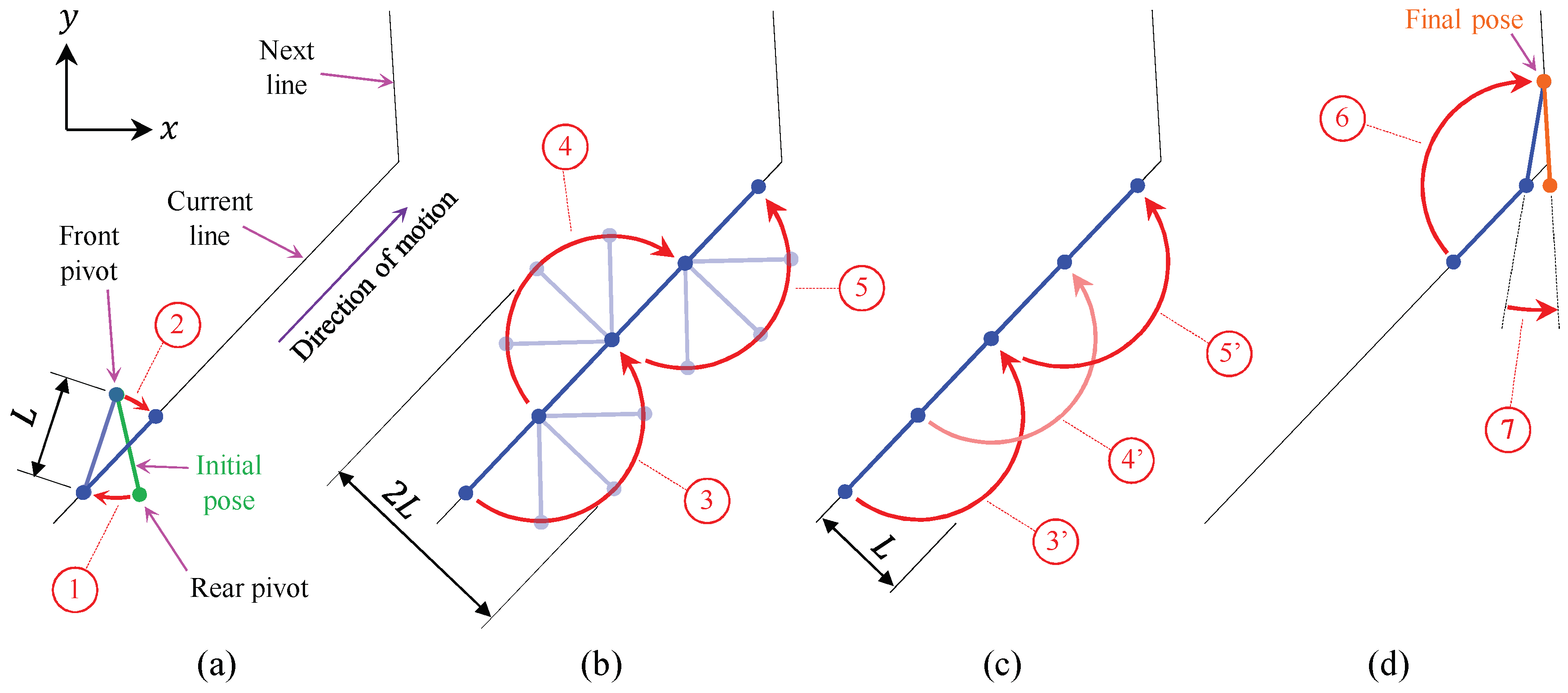
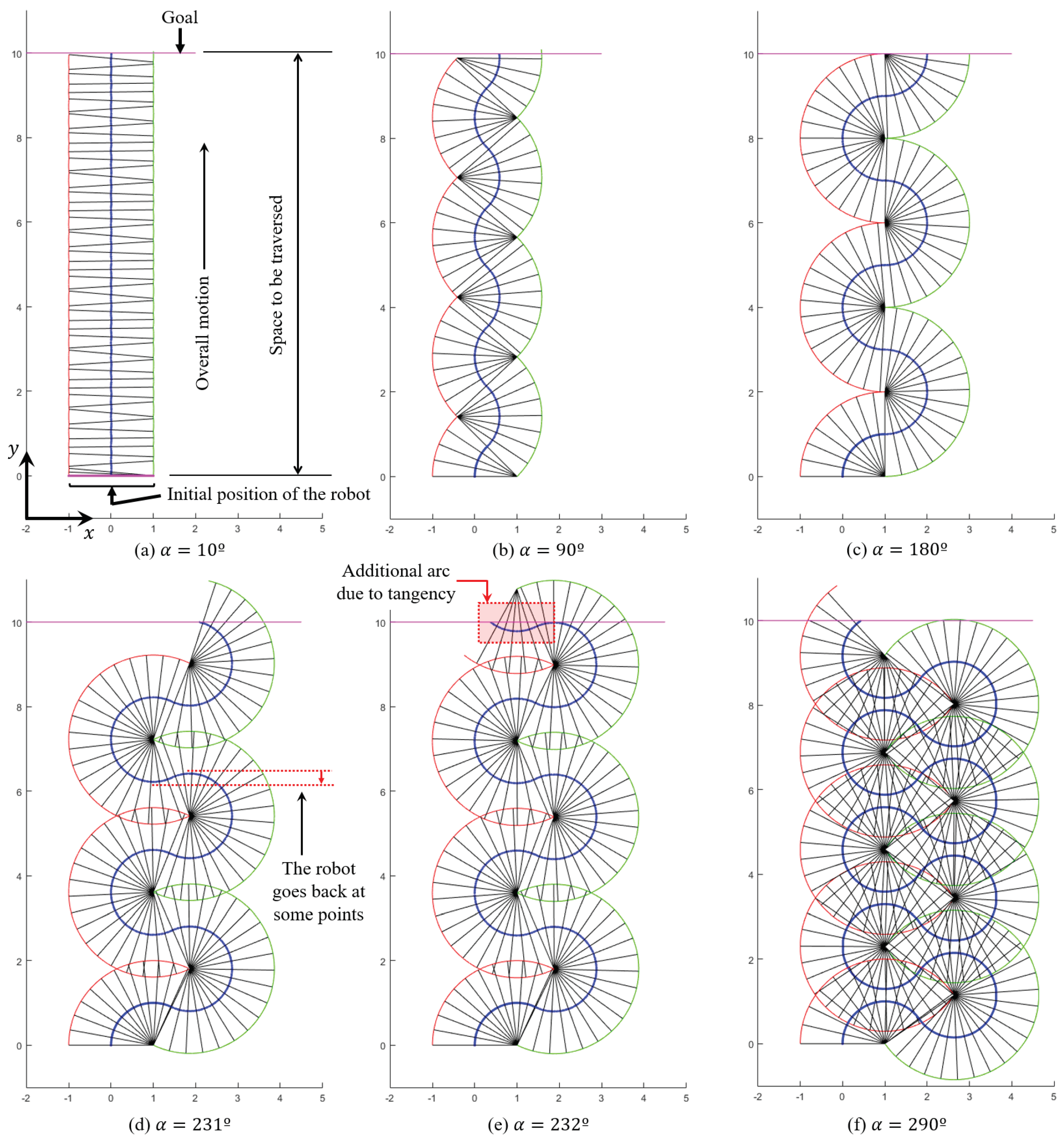
The first decision to make is the gait that the robot should use for following straight trajectories that have no restrictions that is, paths with no obstacles or collisions that may constrain the amplitude of the rotations of the robot (at most, only changes of direction are found). If the motion of the robot is not constrained, then the most reasonable gait for the robot should be based on 180° turns, since they achieve a maximum displacement along the direction of the trajectory and reduce overall time. This choice is illustrated in
Figure 5b,c, and will be further discussed in
Section 4.1.
We assume that, at the beginning of the polygonal path, the robot starts with any orientation, and with its middle point placed on the first straight segment of the path. If this was not the case, it will simply be necessary to rotate the robot around any of its pivots until its center point intersects this segment—or, in case the center point does not intersect the initial segment, a virtual segment may be defined between the center of the robot and the closest point of the first actual segment of the trajectory, continuing then, as explained next, without any changes.
To start the movement that traverses each segment using 180° turns, the robot must be completely aligned with the straight line. In general, the pivots may not be initially on the line. Therefore, two rotations are required for reaching the desired initial pose, as explained next.
3.1.1. Initial Reorientation
As mentioned before, initially, it may be possible that both pivots are not on the line; in that case, the robot must re-orient itself to align with the straight line, with both pivots on it. Two rotations will be needed, as illustrated in
Figure 5a: one rotation about the front pivot (i.e., the one closest to the end of the segment to traverse) and another about the rear pivot.
The first rotation, considered as initial re-orientation and identified in
Figure 5a by the number 1, is based on the search of a point on the line whose distance to the front pivot is equal to the length
L of the robot. This point is found solving the intersection between the line and the circle centered at the front pivot and with radius
L.
After computing the intersection point, through the law of cosines, we calculate the value of the rotation angle 1 (shown in
Figure 5a), which places the rear pivot on the line by rotating the whole robot about the front pivot. Considering the straight line as a vector, with its end at the goal of the motion, if the front pivot is located to the right of this vector, the rotation angle will be positive (counter-clockwise). Otherwise, it will be negative (clockwise), as in
Figure 5a.
After this rotation, a second re-orientation is produced in order to completely align the robot with the line. The second rotation is about the rear pivot (which is already placed on the line) and is identified in
Figure 5a by rotation number 2. The angle to rotate will simply be the angle formed between the robot and the
x-axis, minus the angle formed between the line and the
x-axis.
3.1.2. Straight Motion and Change of Direction
When the robot is completely on the line, the movement along it can begin. As we previously argued, this movement is based on 180° rotations about alternating pivots, alternating the sign of the rotation with each pivot change, as illustrated by rotations {3,4,5} in
Figure 5b. Alternatively, the sign of the rotations may remain constant during the motion, as shown by rotations {3’,4’,5’} in
Figure 5c. If this sign is switched together with the pivots (
Figure 5b), the trajectory is more symmetric with respect to the line to be followed, but it requires twice the space than by keeping the sign of the rotations (
Figure 5c) constant, measuring this space in the direction perpendicular to the line. If there are no space limitations, either gait shown in
Figure 5b,c would be valid.
After performing a certain number of 180° rotations, when the front pivot is sufficiently close to the end of the current line, the robot considers that it has reached the end of the line and starts a sequence of movements for moving to the next straight line (
Figure 5d). The first movement places the rear pivot of the robot on the next line by rotating about the front pivot. The angle to rotate in this case (angle 6 in
Figure 5d) is determined by finding again the intersection point between the new line and a circle centered at the front pivot and with radius
L.
Finally, in order to completely align the robot with the new line, it must be rotated by angle 7 of
Figure 5d about the front pivot (which lies already on the new line). This final angle is again computed as the difference of the angles formed by the robot and the line with the
x-axis. When this change of direction is over, the robot will be able to continue along the new line with the described locomotion: performing 180° turns until the end of the new line is reached, then changing again the direction of motion, etc., until the end of the whole polygonal path is reached.
3.2. Problem 2: Traversing Narrow Corridors
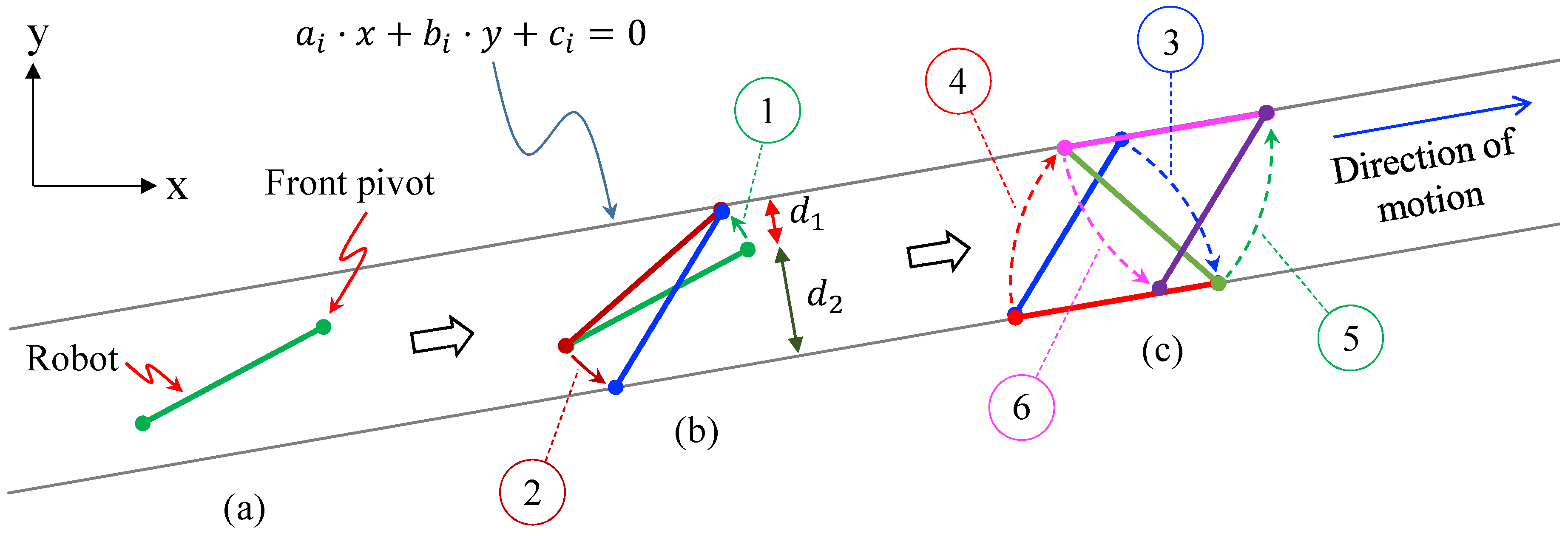
This section focuses on solving those situations where the robot needs to traverse a narrow corridor defined by two parallel walls (
Figure 6), such that the separation between these walls is smaller than the length
L of the robot (otherwise, the robot would be able to traverse the corridor by employing the locomotion illustrated in
Figure 5c). Note that these walls may be actual physical walls, but also virtual walls defined artificially for safety reasons, so that the robot does not collide with other obstacles whose shape may be more involved.
In this scenario, the robot cannot perform complete rotations of 180° and it must use an alternative locomotion, which we explain next. In order to perform the optimal locomotion to traverse a narrow corridor, it will be necessary to perform an initial reorientation of the robot first, so that each pivot is placed on a different wall of the corridor, as explained next.
3.2.1. Initial Maneuvering inside the Narrow Corridor
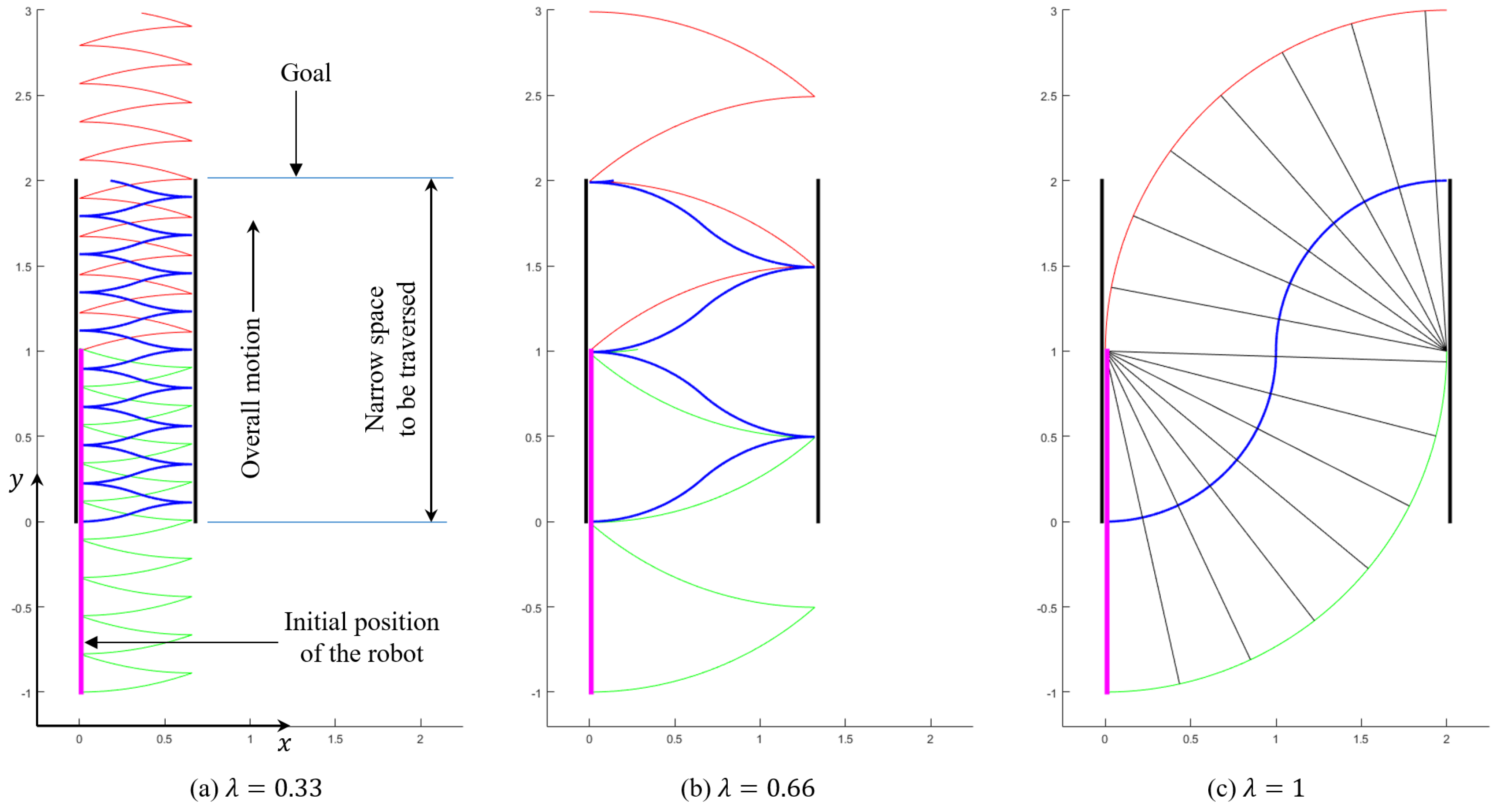
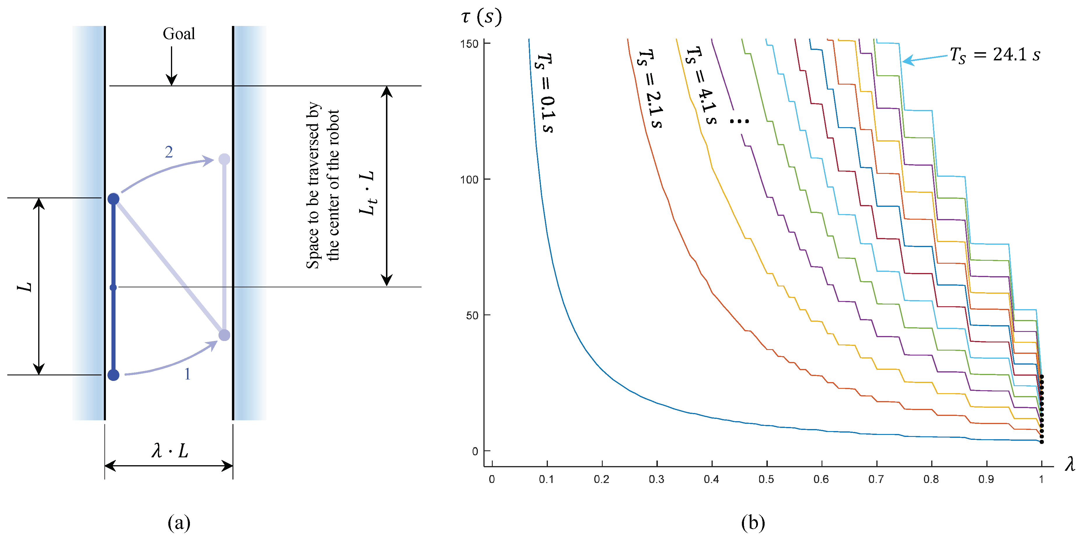
The fastest and more efficient motion for going through a narrow corridor is the one in which the robot moves by placing its whole body alternately on a different wall, as illustrated in
Figure 6c. This motion is the best option since it achieves the maximum displacement in the direction of the corridor during each step. To achieve this motion, the robot must start with each pivot placed on a different wall. The main objective of this sub-section is to determine the pair of rotations that the robot must perform (with each rotation about a different pivot) to reach the desired initial pose (
Figure 6b).
This process begins by looking for the shortest distance
from each wall to the front pivot of the robot:
where each wall
is modeled by a line defined by its implicit equation
. Once the calculation is done, the shortest distance identifies the wall closest to the front pivot, which must be moved to that wall by rotating about the rear pivot (rotation number 1 in
Figure 6b). This rotation is determined by finding the intersection between the closest wall and a circle centered at the rear pivot and with radius
L (where
L is the length of the robot). After obtaining this intersection point, the law of cosines is applied for obtaining the desired angle that the robot must be rotated about the rear pivot in order to place the front pivot at the calculated intersection point.
When this point is reached by the front pivot, the same process needs to be done again for placing the rear pivot on the opposite wall, this time rotating about the front pivot (rotation 2 in
Figure 6b).
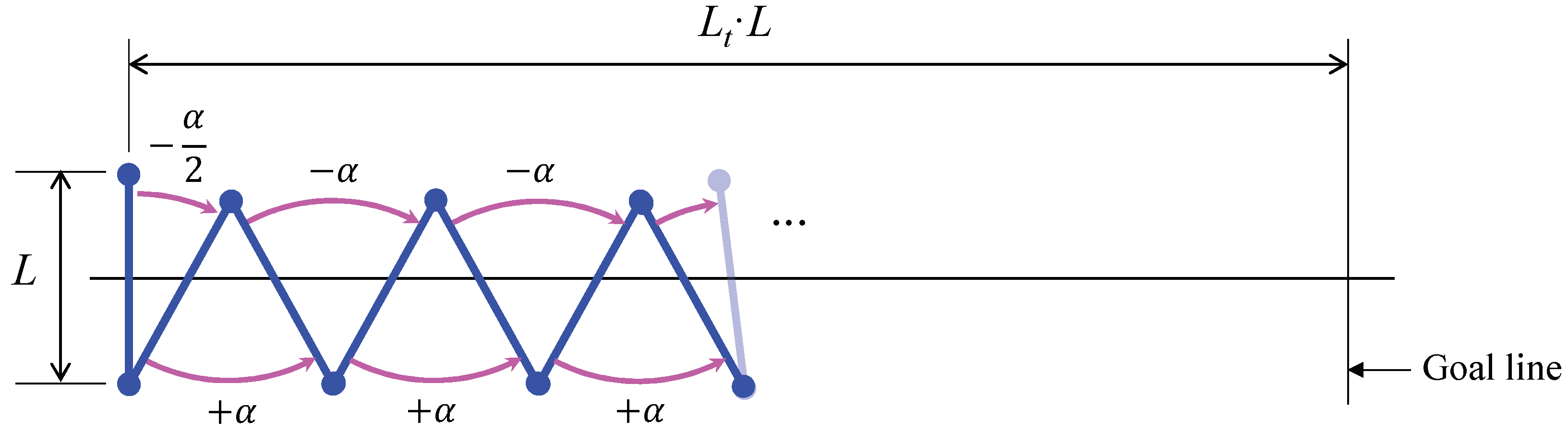
3.2.2. Movement along the Corridor
After each pivot of the robot lies on a different wall, the robot proceeds to move inside the corridor, until reaching its end. This movement is accomplished by rotating always by the same angle, which is the angle formed between the robot and the walls when the robot has each pivot placed on a different wall. As explained before, this is the optimal rotation for advancing along the narrow corridor since it produces the maximum advance along the direction of the corridor in a single rotation. The fixed pivot must be switched after each rotation, whereas the sign of the rotation must be switched every two rotations. This process is illustrated in
Figure 6c, with a sequence of rotations {3,4,5,6}.
3.3. Problem 3: Combination of Both Problems
After explaining the previous two problems (following obstacle-free polygonal trajectories in
Section 3.1, and traversing narrow corridors in
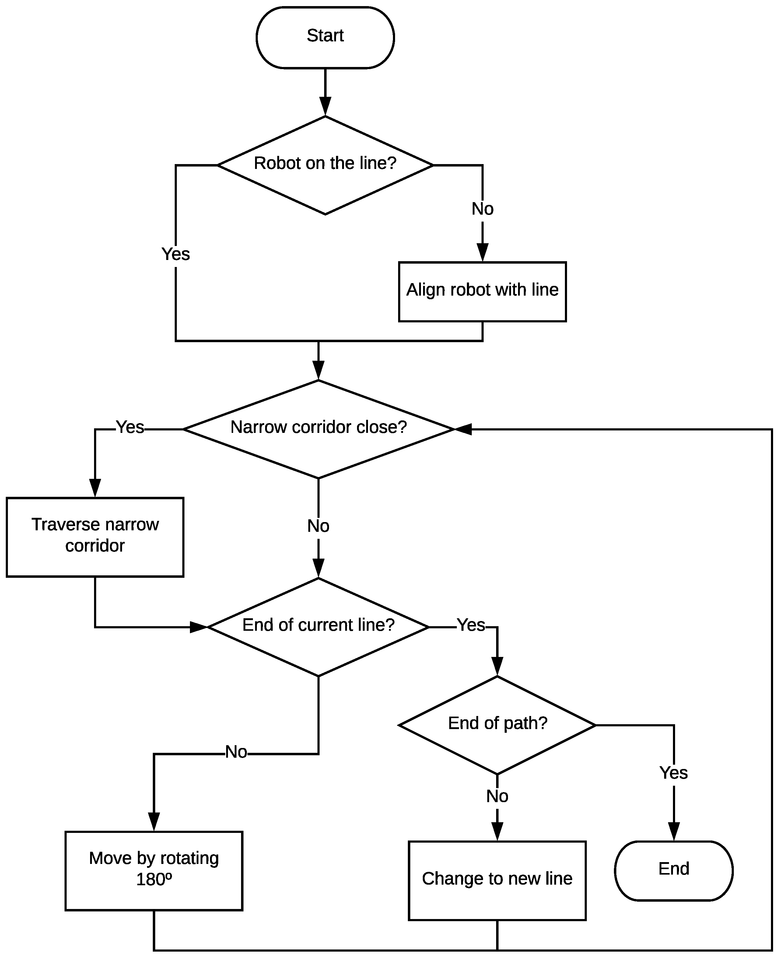
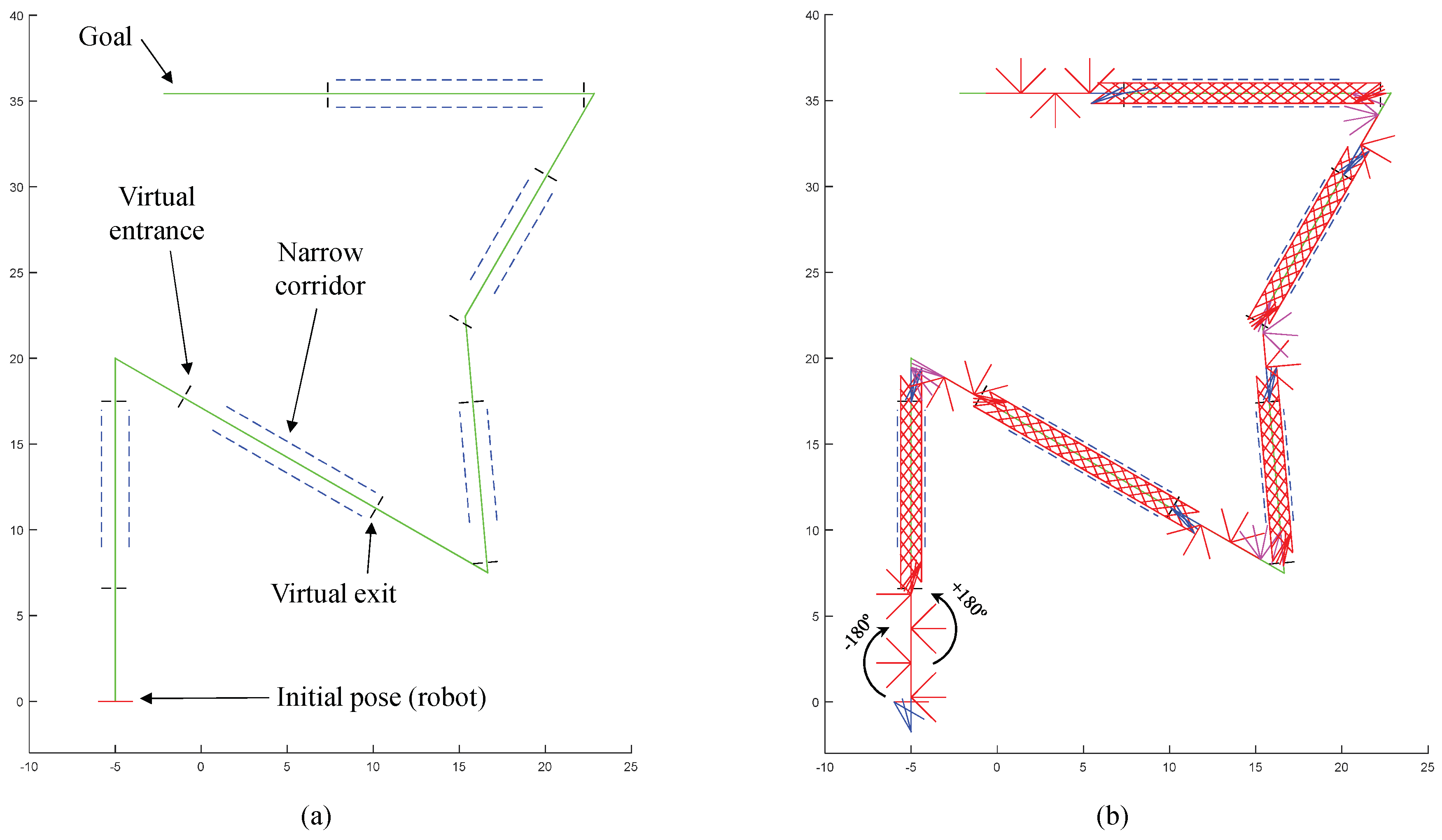
Section 3.2), this section analyzes the combined scenario, in which the robot must follow a polygonal trajectory that has narrow sections. This combination of the two problems is based on an online management by the robot while moving, i.e., as it proceeds along the trajectory, if the robot finds a narrow corridor, a change of direction, or obstacle-free lines, it will perform some or other relevant actions defined in previous subsections. The algorithm used by the robot to manage the different possibilities is illustrated graphically in the flow diagram shown in
Figure 7. This flow diagram describes how the different methods and procedures presented in
Section 3 are “activated” and executed as the robot advances along the trajectory and encounters an obstacle-free straight segment, a narrow corridor, or a change of line.
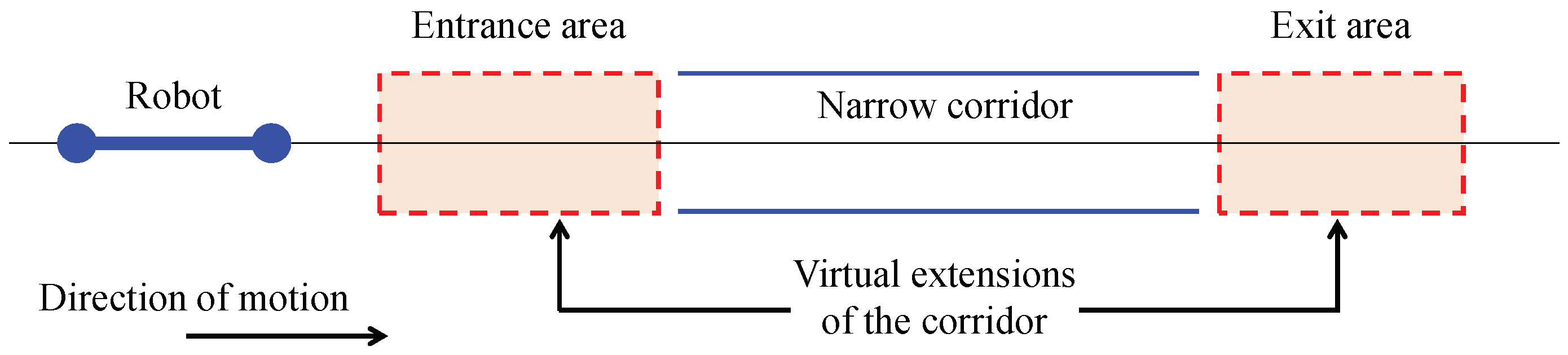
At this point, it is important to specify how the robot is able to face narrow corridors, that is, how it enters and leaves them. In order to solve this situation, virtual narrow areas are defined both at the beginning and at the end of the corridor. These virtual areas will be virtual extensions of the real corridor, as illustrated in
Figure 8.
On the one hand, in order to enter the corridor, when the front pivot enters the first virtual area (denoted by “Entrance area” in
Figure 8), the robot will understand that the corridor is near. Then, it will behave as if it was already inside of the corridor: the robot will perform the corresponding movements for placing its pivots on each virtual wall (as in
Figure 6b), and, afterwards, it will move forward using the gait of
Figure 6c, even if it is still in the virtual entrance of the corridor. In this way, it is guaranteed that the robot will not try to approach the entrance of the corridor by performing wide rotations of 180°, which may produce the collision with the walls of the corridor before entering it.
On the other hand, for leaving the corridor, a similar procedure is followed. This time the robot understands that the narrow corridor is “safely” finished when its rear pivot leaves the second virtual area (denoted by “Exit area” in
Figure 8). Finally, once the robot is completely out, it performs the sequence of movements shown in
Figure 5a in order to completely align with its current straight line, and continue traversing the path.
5. Conclusions and Future Work
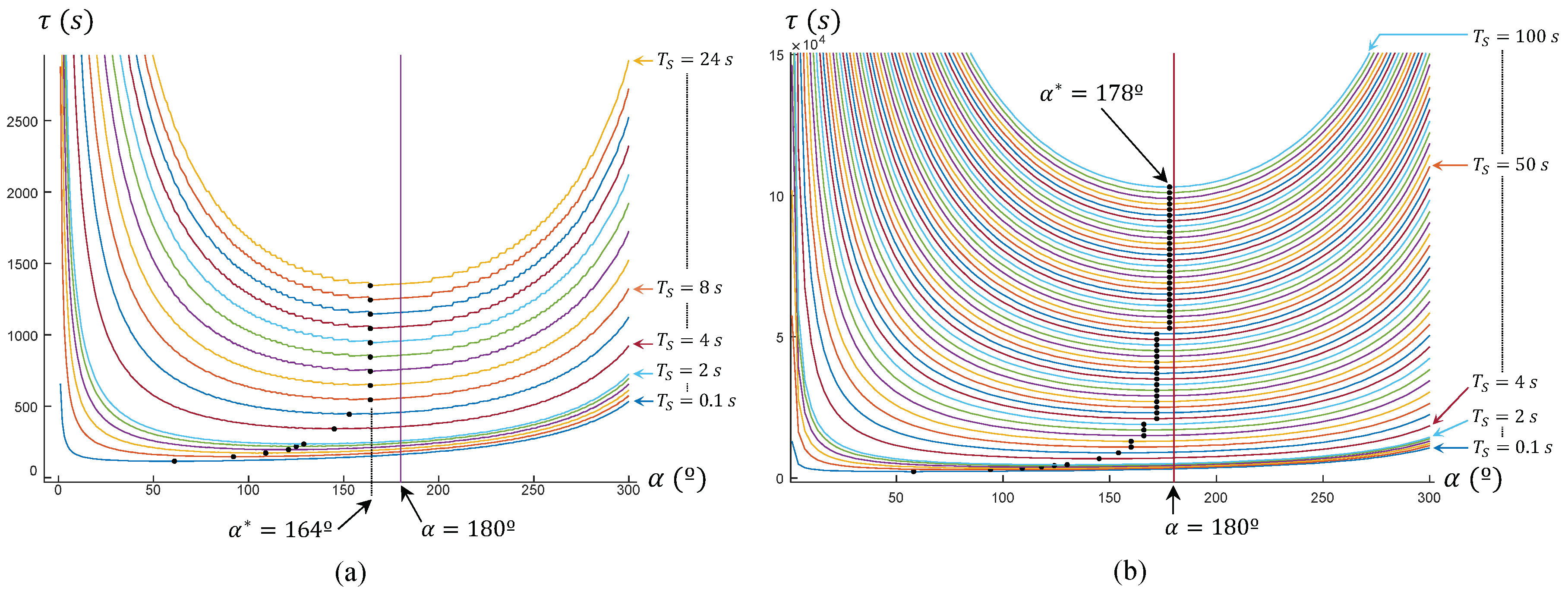
In this paper, we have described the MASAR robot: a new Modular And Single-Actuator Robot. This robot is a type-II SAMR since it has binary adhesion pads that can be adhered or detached from the environment in order to produce the rotation of the robot about different axes, achieving in this way two- or three-dimensional motions using only one continuous actuator. In this paper, we have geometrically solved the planar trajectory tracking problem of this robot when following polygonal trajectories that may have narrow sections that constrain the amplitude of the rotations of the robot. The proposed gait consists in performing 180° rotations when there is no risk of collision between the robot and obstacles of the environment, in order to maximize the distance traveled in a single step. We have shown that, for the MASAR robot, performing rotations of 180° minimizes the time necessary for traversing long trajectories when the time required to switch the adhesion state of the pivots is high. For shorter trajectories and/or pivots that switch their adhesion state quickly, a gait based on rotations of 180° may not be the optimal one, yet it is very close to it. When inside narrow corridors, the proposed gait consists of rotating the robot until both pivots touch the walls of the corridor, since this also maximizes the distance traveled in a single step, subject to the narrowness of the corridor. The analysis of the proposed robot in narrow corridors, however, has shown that this is not the optimal scenario for this robot, since its locomotion mode requires high times to traverse excessively narrow corridors. This can be considered the worst-case scenario in which the proposed robot would need to work, and for this reason it has been analyzed in this paper. Thus, the MASAR robot is most suitable to environments that allow wider rotations for the robot.
Regarding the trajectory-following problem analyzed in this paper, it was addressed from a purely geometric/kinematic perspective, and it assumed polygonal trajectories with narrow sections. In a practical implementation, we may have trajectories with other arbitrary shapes and obstacles, and a purely geometric approach may be insufficient when considering uncertainties of the map or location of the robot, as well as error in tracking of the trajectory (e.g., the robot may not be perfectly aligned with the linear segments of the trajectory, such that the successive rotations of 180° would need to be corrected slightly). In order to cope with all these factors, as part of ongoing and near future work, we are currently approaching the trajectory-following problem of the MASAR robot from a closed-loop control perspective, departing from its velocity model and designing feedback controllers that allow the tracking of arbitrary trajectories, in a similar way to the solutions proposed in [
27] for a differential-drive two-wheeled mobile robot, optimizing time, distance, or energy consumption [
28]. Other ongoing and future tasks to address are: the analysis of trajectories that include concave plane transitions (
Figure 4a), the analysis of the MASAR robot as a modular reconfigurable robot able to perform more complex motions by combining with identical modules (
Figure 4b), and the construction and validation of a prototype of the robot, including the adhesion pads that allow a single module to walk or combine with identical modules (
Figure 3).


