From Single 2D Depth Image to Gripper 6D Pose Estimation: A Fast and Robust Algorithm for Grabbing Objects in Cluttered Scenes ^†

Abstract

In this paper, we investigate the problem of grasping previously unseen objects in unstructured environments which are cluttered with multiple objects. Object geometry, reachability, and force-closure analysis are considered to address this problem. A framework is proposed for grasping unknown objects by localizing contact regions on the contours formed by a set of depth edges generated from a single-view 2D depth image. Specifically, contact regions are determined based on edge geometric features derived from analysis of the depth map data. Finally, the performance of the approach is successfully validated by applying it to scenes with both single and multiple objects, in both simulation and experiments. Using sequential processing in MATLAB running on a 4th-generation Intel Core Desktop, simulation results with the benchmark Object Segmentation Database show that the algorithm takes 281 ms on average to generate the 6D robot pose needed to attach with a pair of viable grasping edges that satisfy reachability and force-closure conditions. Experimental results in the Assistive Robotics Laboratory at UCF using a Kinect One sensor and a Baxter manipulator outfitted with a standard parallel gripper showcase the feasibility of the approach in grasping previously unseen objects from uncontrived multi-object settings.

1. Introduction

A crucial problem in robotics is interacting with known or novel objects in unstructured environments. Among several emerging applications, assistive robotic manipulators seek approaches to assist users to perform a desired object motion in a partial or fully autonomous system. While the convergence of a multitude of research advances is required to address this problem, our goal is to describe a method that employs the robot’s visual perception to identify and execute an appropriate grasp for immobilizing novel objects with respect to a robotic manipulator’s end-effector.

Finding a grasp configuration relevant to a specific task has been an active topic in robotics for the past three decades. In a recent article by Bohg et al. [1], grasp synthesis algorithms are categorized into two main groups, viz., analytical and data-driven. Analytical approaches explore for solutions through kinematic and dynamic formulations [2]. Object and/or robotic hand models are used in [3,4,5,6,7] to develop grasping criteria such as force-closure, stability, and dexterity, and to evaluate if a grasp is satisfying them. The difficulty of modeling a task, high computational costs, and assumptions of the availability of geometric or physical models for the robot are the challenges that analytical approaches deal with in real-world experiments. Furthermore, researchers conducting experiments have inferred that classical metrics are not sufficient to tackle grasping problems in real-world scenarios despite their efficiency in simulation environments [8,9].

On the other hand, data-driven methods retrieve grasps according to their prior knowledge of either the target object, human experience, or through information obtained from acquired data. In line with this definition, Bohg et al. [1] classified data-driven approaches based on the encountered object being considered known, familiar, or unknown to the method. Thus, the main issues relate to how the query object is recognized and then compared with or evaluated by the algorithm’s existing knowledge. As an example, References [10,11,12] assume that all the objects can be modeled by a set of shape primitives such as boxes, cylinders, and cones. During the off-line phase, they assign a desired grasp for each shape while during the on-line phase, these approaches are only supposed to match sensed objects to one of the shape primitives and pick the corresponding grasp. In [13], a probabilistic framework is exploited to estimate the pose of a known object in an unknown scene. Ciocarlie et al. [14] introduced the human operator in the grasp control loop to define a hand postures subspace known as eigen-grasp. This method finds appropriate grasp corresponding to a given task, using the obtained low-dimensional subspace. A group of methods considers the encountered object as a familiar object and employs 2D and/or 3D object features to measure the similarities in shape or texture properties [1]. In [15], a logistic regression model is trained based on labeled data sets and then grasp points for the query object are detected based on the extracted feature vector from a 2D image. The authors in [16] present a model that maps the grasp pose to a success probability; the robot learns the probabilistic model through a set of grasp and drop actions.

The last group of methods, in data-driven approaches, introduce and examine features and heuristics which directly map the acquired data to a set of candidate grasps [1]. They assume sensory data provide either full or partial information of the scene. [17] takes the point cloud and clusters it to a background and an object, then addresses a grasp based on the principal axis of the object. The authors in [18] propose an approach that takes 3D point-cloud and hand geometric parameters as the input, then search for grasp configurations within a lower dimensional space satisfying defined geometric necessary conditions. Jain et al. [19] analyze the surface of every observed point cloud cluster and automatically fit spherical, cylindrical, or box-like shape primitives to them. The method uses a predefined strategy to grasp each shape primitive. The algorithm in [20] builds a virtual elastic surface by moving the camera around the object while computing the grasp configuration in an iterative process. Similarly, [21] approaches the grasping problem through a surface-based exploration. Another approach to grasp planning problem can be performed through object segmentation algorithms to find surface patches [21,22].

In general, knowledge level of the object, accessibility to partial or full shape information of the existing objects in a scene and type of the employed features are the main aspects that characterize data-driven methods. One of the main challenges that most of the data-driven grasping approaches deal with is uncertainties in the measured data which causes failure in real-world experiments. Thus, increasing the robustness of a grasp against uncertainties appearing in the sensed data, or during the execution phase, is the aim for a group of approaches. While [23] uses tactile feedback to adjust the object position deviation from the initial expectation [24] employs visual servoing techniques to facilitate the grasping execution. Another challenge for data-driven approaches is data preparation and specifically background elimination. This matter forces some of the methods to make simplifying assumptions about an object’s situation, e.g., [17] is only validated for objects standing on a planar surface. Finding a feasible grasp configuration subject to the given task and user constraints is required for a group of applications.As discussed by [25,26,27], suggesting desired grasp configurations, in assitive human-robot interaction, results in increasing the users’ engagement and easing the manipulator trajectory adaptation.

In this paper, we introduce an approach to obtain stable grasps using partial depth information for an object of interest. The expected outcome is an executable end-effector 6D pose to grasp the object in an occluded scene. We propose a framework based on the supporting principle that potential contacting regions for a stable grasp can be found by searching for (i) sharp discontinuities and (ii) regions of locally maximal principal curvature in the depth map. In addition to suggestions from empirical evidence, we discuss this principle by applying the concept of wrench convexes. The framework consists of two phases. First, we localize candidate regions, and then we evaluate local geometric features of candidate regions toward satisfying desired grasp features. The key point is that no prior knowledge of objects is used in the grasp planning process; however, the obtained results show that the approach is capable of successfully dealing with objects of different shapes and sizes. We believe that the proposed work is novel and interesting because the description of the visible portion of objects by the aforementioned edges appearing in the depth map facilitates the process of grasp set-point extraction in the same way as image processing methods with the focus on small-size 2D image areas rather than clustering and analyzing huge sets of 3D point-cloud coordinates. In fact, this approach completely sidesteps reconstruction of objects. These features result in low computational costs and make it possible to run the algorithm in near real-time. We also see this approach as a useful solution to obtain grasp configuration according to the given task and user constraints as opposed to most data-driven methods that address this problem by locating the objects and lifting them from the top. Finally, the reliance on only a single-view depth map without the use of color information distinguishes our approach from other candidates in relevant applications. The biggest challenge in the work arises due to uncertainties arising from pixel-wise characteristics; for this matter, relying on larger pixel sets of interest has helped to make the process more robust.

This paper is organized as follows. Grasping preliminaries are presented in Section 2. The grasp problem is stated in Section 3. The proposed approach is presented in Section 4. Specifically, in Section 4.1, we define the object model in the 2D image according to geometry and then introduce the employed grasp model in Section 4.2. Next, in Section 4.3, we propose an approach to find reliable contact regions for the force closure grasp on the targeted object. Details of algorithm implementation for a parallel gripper are provided in Section 5. In Section 6, we validate our proposed approach by considering different scenarios for grasping objects, using a Kinect One sensor and a Baxter robot as a 7-DOF arm manipulator followed by a discussion of the obtained results. Section 7 concludes the paper.

2. Preliminaries

Choosing a stable grasp is one of the key components of a given object manipulation task. According to the adopted terminology from [6], a stable grasp is defined as a grasp having force closure on the object. Force-closure needs the grasp to be disturbance resistance meaning any possible motion of the object is resisted by the contact forces [28]. Thus, determining possible range of force directions and contact locations for robotic fingers is an important part of grasp planning [6]. By considering force-closure as a necessary condition, reference [3] discussed the problem of synthesizing planar grasps. In the planar grasp, all the applied forces will lie in the plane of the object and shape of the object will be the only input through the process. Any contact between fingertips and the object can be described as a convex sum of three primitive contacts.

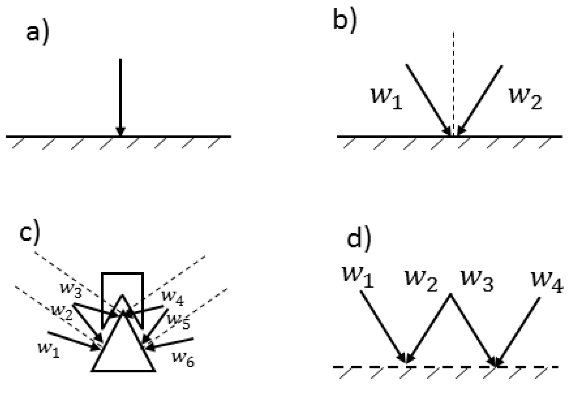
Definition 1.

A wrench convex represents the range of force directions that can be exerted on the object and is determined depending on the contact type and the existing friction coefficient.

Figure 1 shows the primitive contacts and their wrench convexes in 2D. Wrench convexes are illustrated by two arrows forming the angular sector. In the frictionless point contact, the finger can only apply force in the direction of normal. However, through a point contact with friction, the finger can apply any forces pointing into the wrench convex. Soft finger contact can exert pure torques in addition to pure forces inside the wrench convex.

Remark 1.

Any force distribution along an edge contact can be cast to a unique force at some point inside the segment. This force is described by the positive combination of two wrench convexes at the two ends of the contact edge. It is also common in this subject to refer to the wrench convex as friction cone. To resist translation and rotation motions for a 2D object, force-closure is simplified to maintain force-direction closure and torque-closure [3].

Theorem 1.

(Nguyen I) A set of planar wrenches W can generate force in any direction if and only if there exists a set of three wrenches ($w_1$, $w_2$, $w_3$) whose respective force directions $f_1,f_2,$ $f_3$ satisfy: (i) two of the three directions $f_1,f_2,$ $f_3$ are independent. (ii) a strictly positive combination of the three directions is zero: ${\displaystyle \sum _{i=1}^3}{\alpha }_i{f}_i=0$.

Theorem 2.

(Nguyen II) A set of planar forces W can generate clockwise and counterclockwise torques if and only if there exists a set of four forces ($w_1$, $w_2$, $w_3$, $w_4$) such that three of the four forces have lines of action that do not intersect at a common point or at infinity. Let $p_{12}$ (resp. $p_{34}$) be the points where the lines of action of $w_1$ and $w_2$ (resp. $w_3$ and $w_4$) intersect; there exist positive values of ${\alpha }_i$ such that $p_{34}-p_{12}=\pm ({\alpha }_1{f}_1+{\alpha }_2{f}_2)=\mp ({\alpha }_3{f}_3+{\alpha }_4{f}_4).$

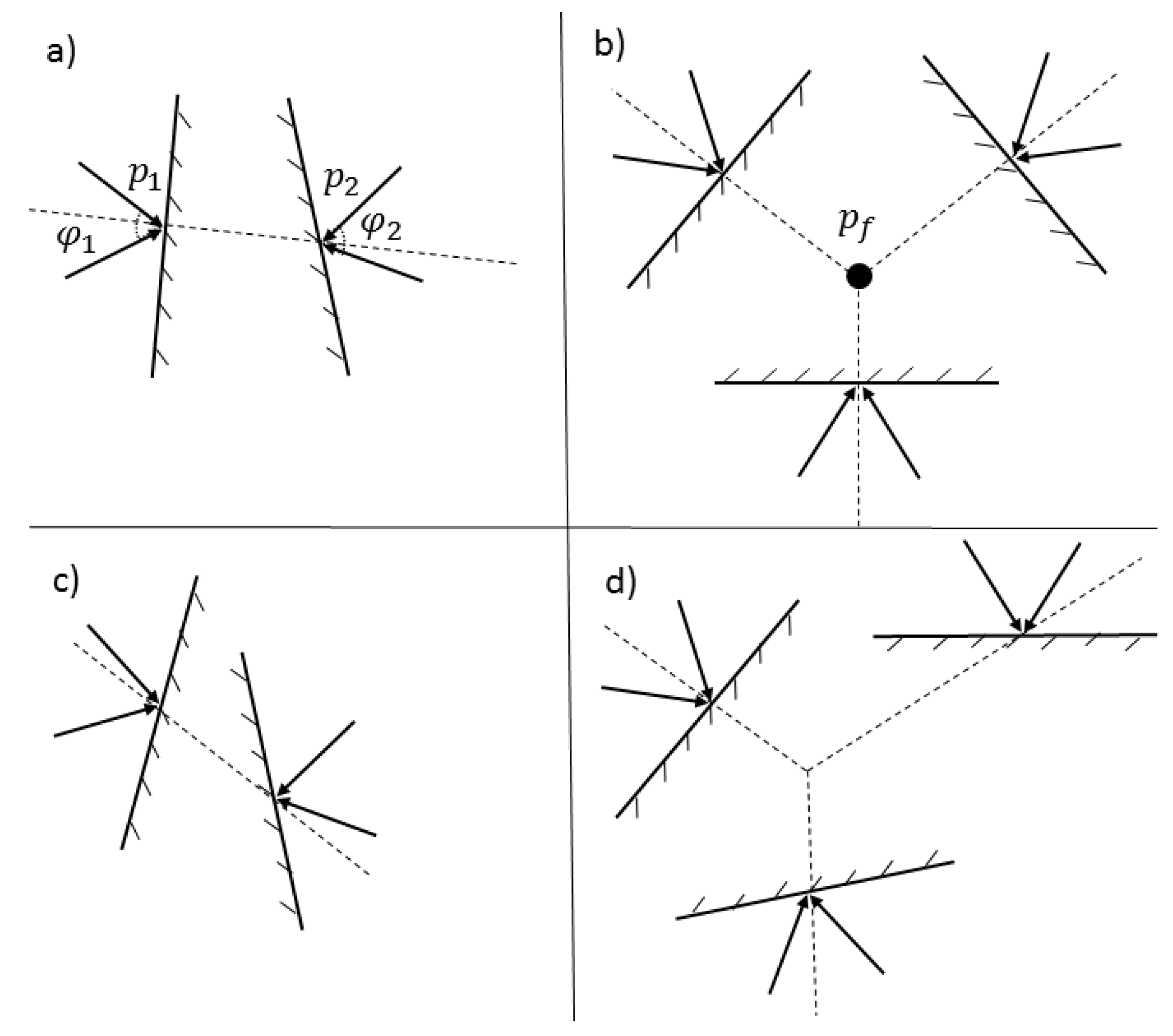
Basically, force-direction closure checks if the contact forces (friction cones) span all the directions in the plane. Torque-closure tests if the combination of all applied forces produces pure torques. According to Theorem I and II, existence of four wrenches with three being independent is necessary for a force-closure grasp in a plane. Assuming the contacts are with friction, each point contact provides two wrenches. Thus, a planar force-closure grasp is possible with at least two contacts with friction. As stated in [3,4], the conditions for forming a planar force-closure grasp with two and three points are interpreted in geometric sense as below and illustrated in Figure 2:

• Two opposing fingers: A grasp by two point contacts, $p_1$ and $p_2$ with friction is in force-closure if and only if the segment $p_1-p_2$ points out of and into two friction cones respectively at $p_1$ and $p_2$. Mathematically speaking, assuming ${\phi }_1$ and ${\phi }_2$ are angular sectors of friction cones at $e_1$ and $e_2$, $arg(p_1-p_2)\in \pm ({\phi }_1\cap -{\phi }_2)$ is the necessary and sufficient condition for two point contacts with friction.
• Triangular grasp: A grasp by three point contacts, $p_1$, $p_2$, and $p_3$ with friction is in force-closure if there exists a point, $p_f$ (force focus point) such that for each $p_i$, the segment $p_f-p_i$ points out of the friction cone of the $i\mathrm{th}$ contact. Let $k_i$ be the unit vector of segment $p_f-p_i$ which points out the edge; a strictly positive combination of the three directions is zero: ${\displaystyle \sum _{i=1}^3}{\alpha }_i{k}_i=0$.

An appropriate object representation and analysis on the shape of objects based on the accessed geometry information is needed to find contact regions for a stable grasp. In Section 4, we relate planar object representation to a proper grasp configuration to obtain an object’s possible grasps.

3. Problem Definition

The problem addressed in this paper is to find contacting regions for grasping unknown objects in a cluttered scene. The obtained grasp needs to exhibit force-closure, be reachable, and feasible under the specifications of a given end-effector. Partial depth information of the object, which is sensed by an RGBD camera, is the only input through this process and the proposed approach assumes that the manipulated objects have rigid and non-deformable shapes. In practice, we do not use objects with transparent and reflective surfaces since they cannot be sensed by the employed sensor technology. We note that we do not address the problem of finger placement of a generalized n-fingered gripper interacting with an arbitrary object. Instead, we focus on identification of reachable points on the surfaces of novel objects in multi-object scenes; these can then be tested for force-closure using existing results in the literature. We only provide an explicit algorithm for locating the fingers of a parallel gripper on previously unseen objects of arbitrary shapes and sizes.

4. Approach

In this section, we first present an object representation and investigate its geometric features based on the scene depth map; then a grasp model for the end-effector is provided. In the end, pursuant to the development, we draw a relationship between an object’s depth edges and force-closure conditions. Finally, we specify contact location and end-effector pose to grasp the target object.

4.1. 2D Object Representation

Generally, 3D scanning approaches require multiple-view scans to construct complete object models. In this work, we restrict our framework to use of partial information captured from a single view and represent objects in a 2-dimensional space. As previously stated, our main premise is that potential contacting regions for a stable grasp can be found by looking for (i) sharp discontinuities or (ii) regions of locally maximal principal curvatures in the depth map. A depth image can be shown by a 2D array of values which is described by an operator $d(.)$

$$z=d(r,c),d(.):R^2\to R$$

(1)

where z denotes the depth value (distance to the camera) of a pixel positioned at coordinates $(r,c)$ in the depth image $\left(I_d\right)$. Mathematically speaking, our principle suggests a search for regions holding high gradient property in depth or depth direction values. Gradient image, gradient magnitude image, and gradient direction image are defined as follows

$$\begin{array}{ccc}\mathrm{Depth}\mathrm{Image}:\hfill & I_d=\hfill & \left[d(r_i,c_i)\right]\hfill \\ \mathrm{Image}\mathrm{Gradient}:\hfill & ▽I=\hfill & {({\displaystyle \frac{\partial I_d}{\partial x}},{\displaystyle \frac{\partial I_d}{\partial y}})}^T\hfill \\ \mathrm{Gradient}\mathrm{Magnitude}\mathrm{Image}:\hfill & I_M=\hfill & [\sqrt{{(\frac{\partial I_d}{\partial x})}^2+{(\frac{\partial I_d}{\partial y})}^2]}\hfill \\ \mathrm{Gradient}\mathrm{Direction}\mathrm{Image}:\hfill & I_{\theta }=\hfill & [{tan}^{-1}((\frac{\partial I_d}{\partial y})/(\frac{\partial I_d}{\partial x}))]\hfill \end{array}$$

(2)

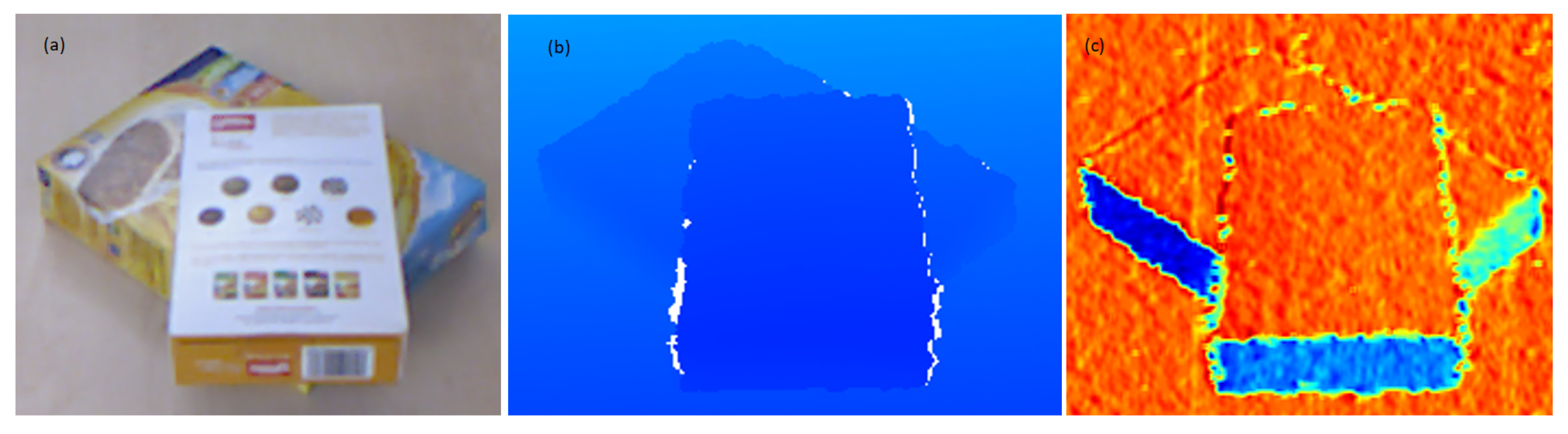
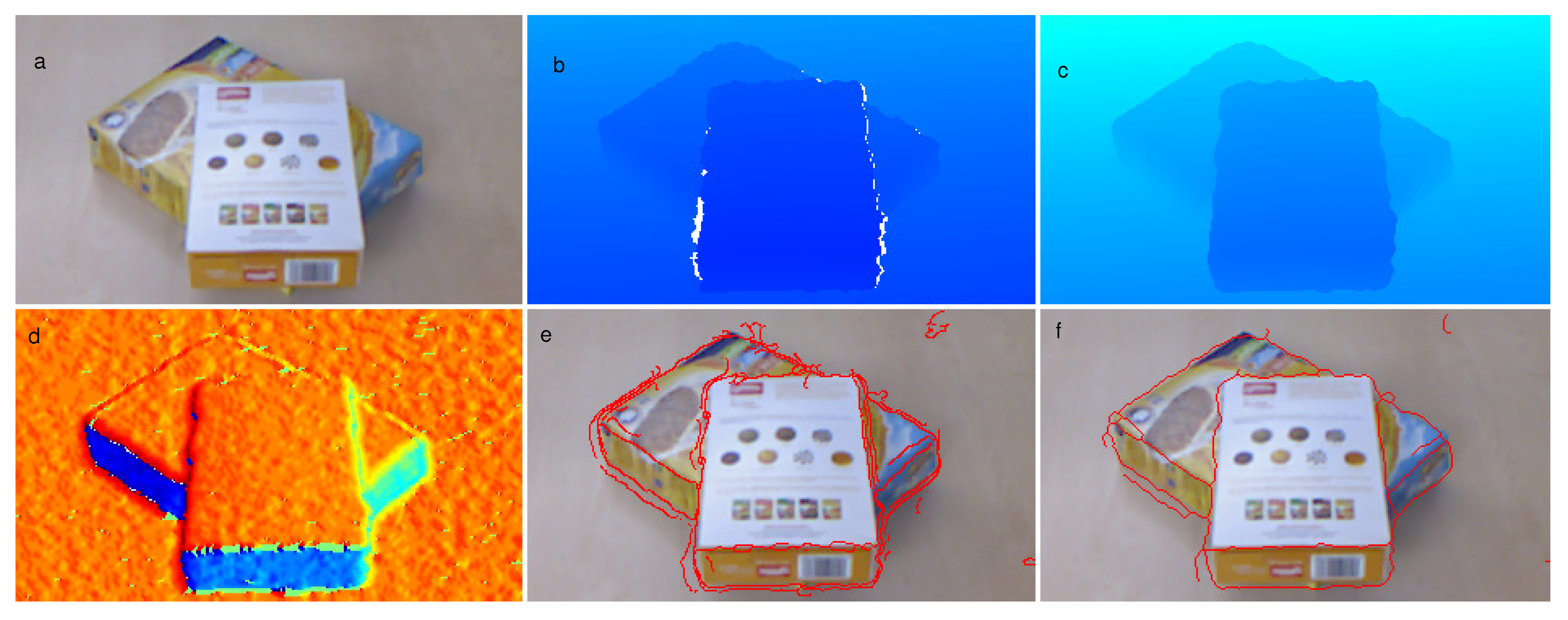
where gradient magnitude image pixels describe the change in depth values in both horizontal and vertical directions. Similarly, each pixel of gradient direction image demonstrates the direction of largest depth value increase. In Figure 3, color maps of depth image and gradient direction image are provided. Sharp change in the color is an indication of occurrence of discontinuity in intensity values. Regions holding these specific features, in the image, locally divide the area into two sides and cause appearance of edges. In our proposed terminology, a depth edge is defined as a 2-dimensional collection of points in the image plane which forms a simple curve and satisfy the high gradient property.

Definition 2.

A point set $p=(x,y)$ in the plane is called a curve or an arc if $x=x\left(t\right)$ and $y=y\left(t\right)$ where $a\le t\le b$ while $x\left(t\right)$ and $y\left(t\right)$ are continuous functions of t. The points $p\left(a\right)$ and $p\left(b\right)$ are said to be initial and terminal points of the curve. A simple curve never crosses itself, except at its endpoints. A closed contour is defined as a piecewise simple curve in which $p\left(t\right)$ is continuous and $p\left(a\right)=p\left(b\right)$. According to the Jordan curve theorem [29], a closed contour divides the plane in two sets, interior and exterior. Therefore, we define surface segment as a 2D region in the image plane which is bounded by a closed contour.

To expound on the kinds of depth edges and what they offer to the grasping problem, we investigate their properties in the depth map. All the depth edges are categorized into two main groups: (1) Depth Discontinuity (DD) edges and (2) Curvature Discontinuity(CD) edges. A DD edge is created by high gradient in depth values or a significant depth value difference between its two sides in the 2D depth map ($I_d$). It intimates a free-space between its belonged surface and its surroundings along the edge. A CD edge emerges from the directional change of depth values ($I_{\theta }$) although it holds a continuous change in depth values on its sides. Please note that the directional change of depth values is equivalent to surface orientation in 3D. In fact, a CD depth edge illustrates intersection of surfaces with different orientation characteristics in 3D. CD edges are further divided into two subtypes, namely concave and convex. A CD edge is called convex if the outer surface of the object curves such as the exterior of a circle in its local neighborhood while it curves such as a circle’s interior in the local neighborhood of a concave edge.

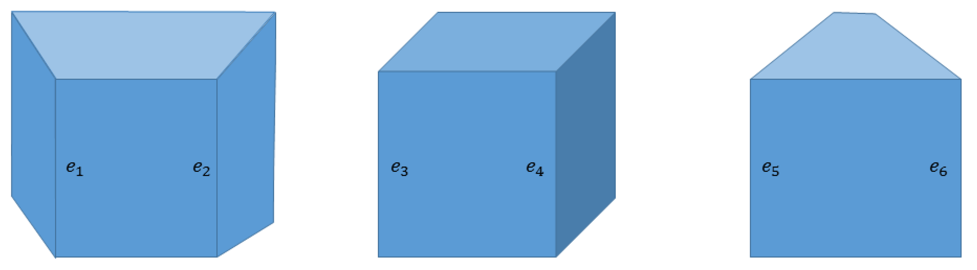
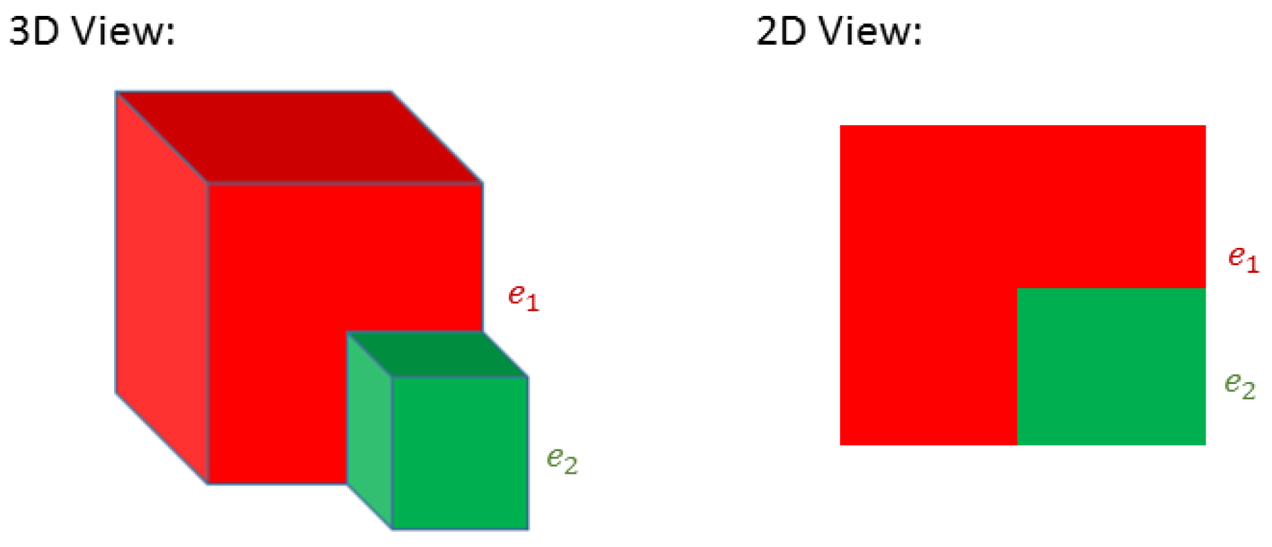
Moreover, each surface segment in the image plane is the projection of an object’s face. In particular, projection of a flat surface maps all the belonged points to the corresponding surface segment while in a case of curved/non-planar face, the corresponding surface segment includes that subset of the face, which is visible in the viewpoint. Assume that operator $\lambda :R^2\to R^3$ maps 2D pixels to their real 3D coordinates. In Figure 4, the $S_i$ show 2D surface segments and $A_i$ indicate collections of 3D points. It is clear that $S_1$ represents a flat face of the cube and $\lambda \left(S_1\right)=A_1$ while the surface segment $S_2$ implies only a subset of the cylinder’s lateral surface in 3D bounded between $e_2$ and $e_4$ such that $\lambda \left(S_2\right)\subseteq A_2$. Hence, a depth edge in the image plane may or may not represent an actual edge of the object in 3-dimensional space. Thus, edge type determination, in the proposed framework, relies on the viewpoint. While a concave CD edge holds its type in all the viewpoints, a convex CD edge may switch to DD edge and vice versa by changing the point of view.

4.2. Grasp and Contact Model

Generally, a precision grasp is indicated by end-effector and fingertips poses with respect to a fixed coordinate system. According to terminology adopted from [30], referring to an end-effector E with $n_E$ fingers and $n_{\theta }$ joints with the fingertips contacting an object’s surface, a grasp configuration, G, is addressed as follows:

$$G=(p_G,{\theta }_G,C_G)$$

(3)

where $p_G$ is the end-effector pose (position and orientation) relative to the object, ${\theta }_G=({\theta }_1,{\theta }_2,\dots ,{\theta }_{n\theta })$ indicates the end-effector’s joint configuration, and $C_G={\{c_i\in S\left(O\right)\}}_{i=1}^{n_E}$ determines $n_E$ point contacts on the object’s surface. The contact locations set on the end-effector’s fingers is $C_E={\{{\overline{c}}_i\in S\left(E\right)\}}_{i=1}^{n_E}$ and is obtained by a forward kinematics derived from the end-effector joint configuration ${\theta }_G$.

Throughout this paper, we make an assumption regarding the end-effector during the interaction with the object. Each fingertip applies a force in the direction of its normal and the forces exerted by all fingertips lie in the same plane. We refer to this plane and its normal direction, respectively, as end-effector’s approach plane, ${\rho }_G$, and approach direction, ${\overrightarrow{V}}_G$. In addition, some of the end-effector geometric features, such as finger’s opening-closing range, can be described according to how they appear on the approach plane. 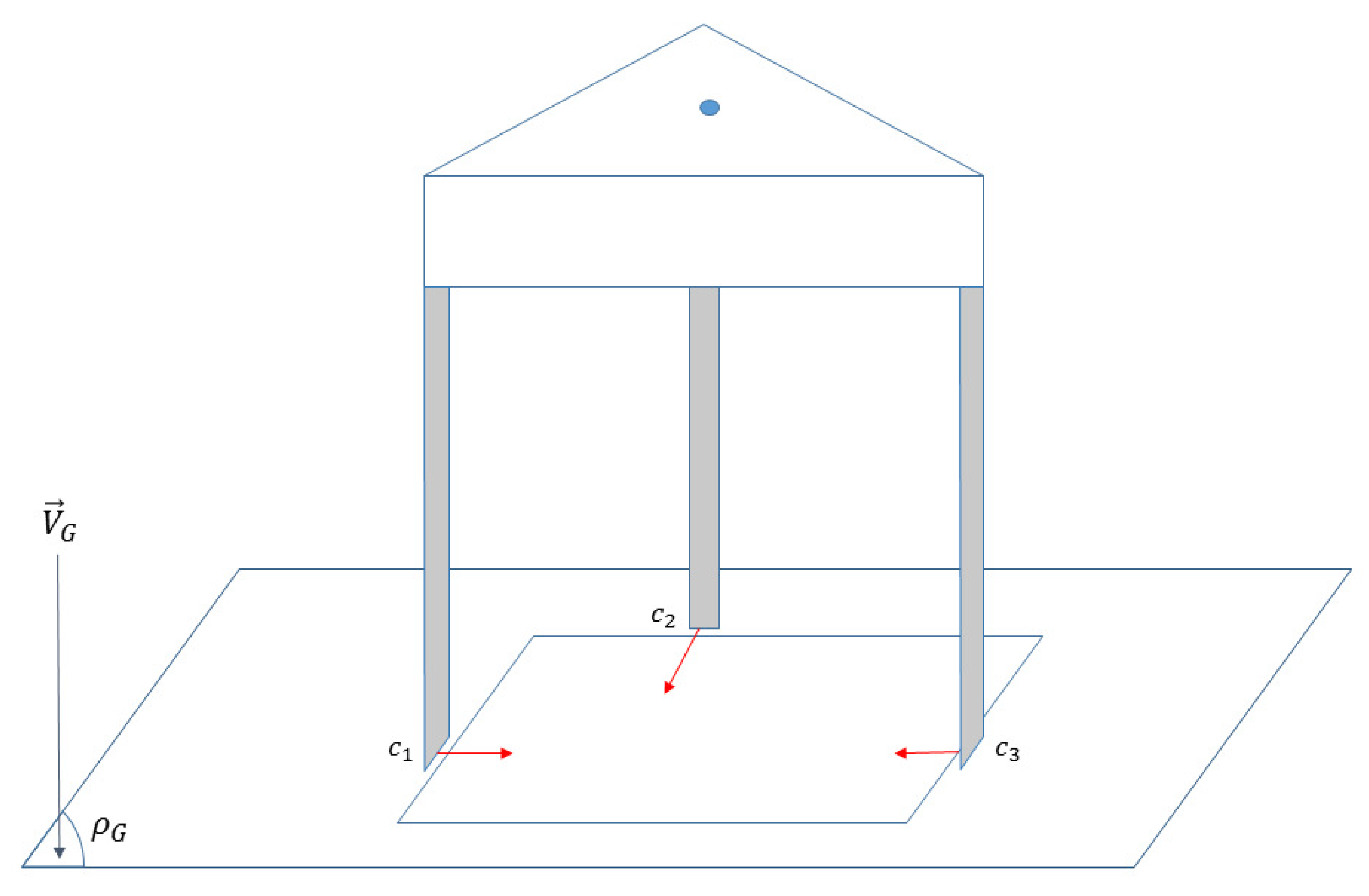Figure 5 shows how a three-finger end-effector contacts points $c_1$, $c_2$, and $c_3$ to grasp the planar shape.

4.3. Edge-Level Grasping

Until this point, we have discussed how to extract depth edges and form closed contours based on the available partial information. In other words, objects are captured through 2D shapes formed by depth edges. Experiments show human tendency to grasp the objects by contacting its edges and corners [3]. The main reason is that edges provide a larger wrench convex and accordingly a greater capability to apply necessary force and torque directions. In this part, we aim to evaluate existence of grasps for each of the obtained closed contours as a way to contact an object. For this matter, we use contours as the input for the planar grasp synthesis process. The output grasp will satisfy reachability, force-closure, and feasibility with respect to end-effector geometric properties. Next, we describe how the 6D pose of the end-effector is obtained from contact points specified on the depth image. Finally, we point out the emerging ambiguity and uncertainties due to the 2D representation.

If we assume that the corresponding 3D coordinates of a closed contour are located on a plane, planar grasp helps us to find appropriate force directions lying on this virtual plane. In addition, edge type determination guides us to evaluate the feasibility of applying the force directions in 3D. Reachability of a depth edge is measured by the availability of a wrench convex lying in the plane of interest. A convex CD edge provides wrench convexes for possible contacting of two virtual planes while a concave CD edge is not reachable for a planar grasp. Exerting force on a DD edge, which also points to object interior, is just possible from one side. Therefore, DD and convex CD edges are remarked as reachable edges while concave CD edges are not considered to be available points for planar contact.

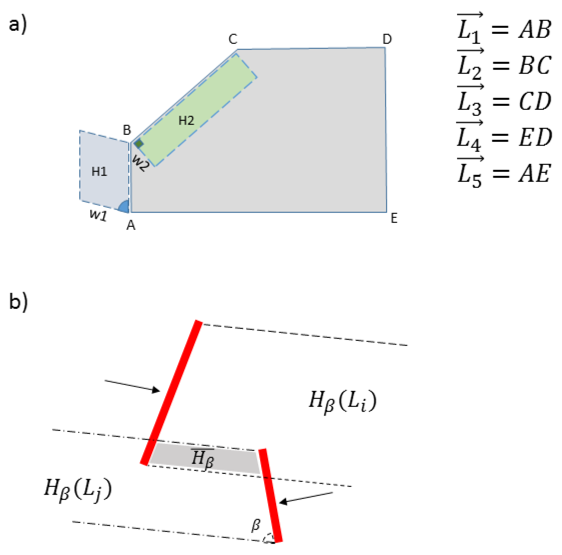
For simplicity in the analysis and without loss of generality, we approximate curved edges by a set of line segments. As a result, all 2D contours turn into polygonal shapes. To obtain the planar force-closure grasp, we assume each polygon side represents just one potential contact. Then we evaluate all the possible combinations of polygon sides subject to the force-direction closure (Theorem 1) and torque-closure (Theorem 2) conditions.

We name the validation of force-direction closure, Angle test. According to Section 2, force-direction closure is satisfied for a two-opposing-fingers contact if the angle made by two edges is less than twice the friction angle. The Angle test for a three-finger end-effector is passed for a set of three contacts such that a wrench from the first contact with opposite direction overlaps with any positive combination of the other two contacts’ provided wrenches (friction cones) [4].

In Section 2, we also discussed how to check if a set of points, corresponding to wrench convexes, satisfy the torque-closure condition. Here, we apply the following steps to recognize regions that include such points on each edge:

• Form orthogonal projection areas ($H_i$) for each edge $e_i$.
• Find the intersection of projection areas by the candidate edges and output the overlapping area ($\overline{H}$).
• Back-project the overlapping area on each edge and output the contact regions (${\overline{e}}_i$).

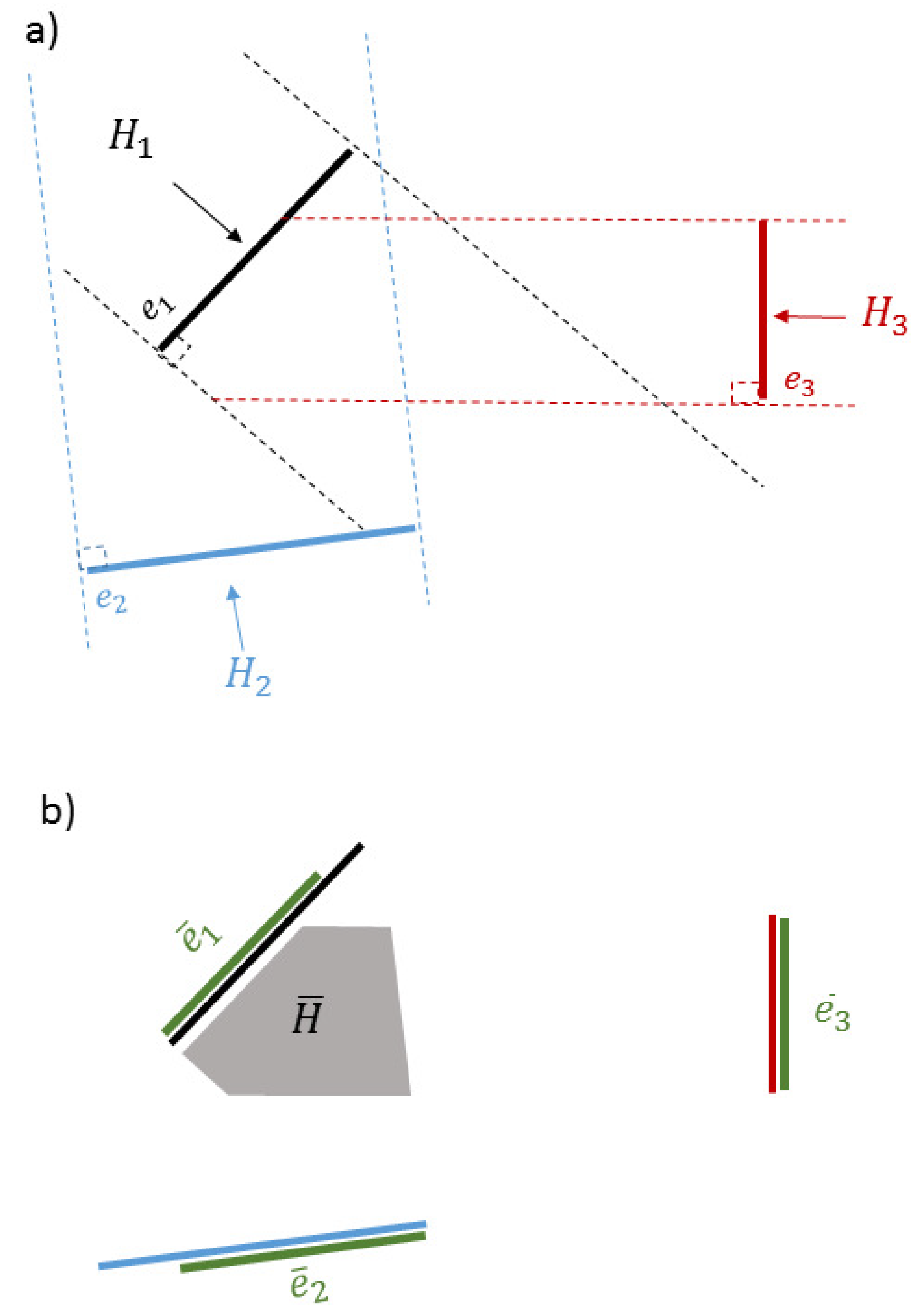
In fact, torque-closure is satisfied if there exists a contact region for each edge. We call this procedure Overlapping Test. Figure 6 illustrates this for a grasp using a combination of 3 reachable edges detected for an object. Specifically, Figure 6a illustrates projection areas for each edge by color coded dashed lines, while in Figure 6b, the shaded region corresponds to the overlapping area and green lines correspond to acceptable contact regions.

Please note that the entire procedure up to this point is performed in the image plane. In the next step, we extract 3D coordinates of the involved edges in order to evaluate the feasibility of the output grasp with respect to the employed end-effector. For instance, comparison of Euclidean distance of line segments and two-fingered gripper width range specifies if the end-effector can fit around a pair of edges. Furthermore, by accessing the 3D coordinates of pixels, we find the Cartesian equation of a plane passing through the edge contact regions (${\overline{e}}_i$). According to Section 4.2, the obtained plane determines end-effector approach plane (${\rho }_G$) and approach direction (${\overrightarrow{V}}_G$) at the grasping moment. To make the grasp robust to positioning errors, the center of each usable edge contact region ($e_i^{*}$) is chosen as the point contact on the object’s surface ($c_i$). It is beyond the scope of this paper to completely specify grasp configuration $G($$p_G,$${\theta }_G,$ $C_G)$ for an arbitrary object being grasped with a generalized multi-fingered gripper. To completely specify G, one needs to specify end-effector kinematics and a chosen grasp policy for execution. While necessary and sufficient conditions for two and three-finger force-closure grasps are provided in Section 2, a complete grasp specification for a parallel gripper is provided in Section 5.

To sum up our proposed approach, Figure 7 presents a block diagram that shows how the process is applied to an input depth image to output a desired 6D gripper pose. The approach is split into two main parts. During contact region localization process, all the depth edges are extracted from the input. After a post-processing step, closed contours are formed and each edge gets an edge type feature (CD/DD). By filtering out concave CD edges, available contact points alongside corresponding force directions are provided to second section of the approach. In the Force-closure Grasp Synthesis, depending on the desired number of contacts, all the possible combinations of edge segments are constructed. Force direction closure and torque-closure are validated by applying Angle Test and Overlap Test on each constructed combination. These two tests are derived from Theorems 1 and 2 in Preliminaries Section and are specifically described for a parallel gripper in the Implementation Section. The combinations that satisfy force-closure conditions are subject to the last two constraints, namely plane existence and gripper specifications. Usable edge segment centers determine fingers’ contacting point while the normal to the plane described by these points specifies the end-effector approach direction. Based on the kinematic model of the end-effector and chosen grasp policy, its 6D pose at the grasping moment is calculated for each candidate grasp. The following pseudo-code summarizes the various steps for constructing a force-closure grasp using a depth image:

• detect disc edges from depth image
• detect curvature disc edges from gradient direction image
• form closed 2D contours using all depth edges from Steps 1 and 2
• for each contour:

  (a)

  approximate curved edges by line segments to obtain corresponding polygon

  (b)

  remove the concave CD edges to obtain reachable edges

  (c)

  make combination of edges with desired number of contacts (depending on available number of fingers)

  (d)

  for each edge combination:

  • perform Angle Test (based on Theorem 1)
  • perform Overlapping Test (based on Theorem 2) and output edge contact regions in 2D
  • perform end-effector geometric constraint test and output end-effector approach plane and contact points
  • output grasp parameters given end-effector kinematics

It is worth mentioning the possible uncertainties in our method. Throughout this paper, we assume that friction between fingertips and the object is large enough such that applied planar forces lie inside the 3D friction cones at the contacting points. To clarify, the current layout of our approach provides similar grasps for the contact pairs $(e_1,e_2)$, $(e_3,e_4)$ and $(e_5,e_6)$ in Figure 8; however, the depth edges in these three cases offer different 3D wrench convexes which increases the grasping uncertainty. Another impacting factor is the relative position of force focus point with respect to the center of gravity of the object. Hence, we assume that a sufficient level of force is available to prevent any possible torques arising from this uncertainty.

5. Implementation for Parallel Gripper

In this section, we describe the implementation steps to process a depth image as the input and identify appropriate grasps for a two-opposing-finger gripper. Therefore, we employ the described algorithm in Section 4.3 to construct a grasp based on forming a combination of two edges to indicate a pair of contact locations. A set of pixel-wise techniques is used to achieve the regions of interest in a 2D image and eventually obtain the desired 3D grasp. In addition, to cope with noise effects of edge detection step in the algorithm, we use a tweaked procedure to follow the approach steps. In fact, we skip contour formation process in the third step of the approach and directly look for the pairs that meet the discussed conditions. Thus, if an edge is missed in the detection step, we do not lose the whole contour and its corresponding edge pairs. However, this results in expansion of the pair formation search space; therefore, later, in this section, we introduce constraints to restrict this search space.

5.1. Edge Detection and Line Segmentation

According to Section 4.1, depth edges appear in depth image and gradient direction image. Due to the discontinuity existing by traveling in the orthogonal direction of a DD edge in depth image ($I_d$), the pixels belonging to the edge are local maxima of $I_M$ (magnitude of the gradient image $▽I$). Alongside, a CD edge demonstrates a discontinuity in gradient direction image ($I_{\theta }$) values, which illustrate a sudden change in normal directions corresponding to the edge neighborhood. Thus, in the first step, an edge detection method is required to be applied to $I_d$ and $I_{\theta }$ to capture all the DD and CD edges, respectively. We selected Canny edge detection method [31] that outputs the most satisfying results with our collected data.

Generally, the output of an edge detection method is a 2D binary image. Imperfect measurement in depth image yields appearance of artifacts and distorted texture in the output binary images. For instance, an ideal edge is marked out with one pixel-width. However, practically there exist non-uniform thickness along the detected edges. To reduce such effects and enhance the output of edge detection, a set of morphological operations is applied to the binary images. In coordination with the aforementioned attempt, logical OR operation is used to integrate all the marked pixels corresponding to depth edges from $I_d$ and $I_{\theta }$ in a single binary image called detected depth image $I_{DE}$. Figure 9 shows the output of edge detection step for an acquired depth image from the Object Segmentation Dataset [32]. Note that the only input through the whole algorithm is $I_d,$ and color image is merely used to visualize the obtained results. For visualizing, a range of colors is also assigned to the values of $I_d$ and $I_{\theta }$. Improvements made by the morphological operations is noticeable in Figure 9d.

To perform further processing, a procedure is required to distinguish edges by a 2D representation in the obtained binary image ($I_{DE}$). Considering a 2D image with the origin on the left bottom corner, each pixel is addressed by a pair of positive integers. We employed a method proposed in [33] to cluster binary pixels into groups and then represent them by start and end points. Given $I_{DE}$, we first congregate the marked pixels into connected pixel arrays such that each pixel in an array is connected only to its 8 immediate neighbor pixels of the same array. Next, an iterative line fitting algorithm is used to divide the pixel arrays into segments such that each segment is indicated by its two endpoints. The pixels belong to a segment, satisfy an allowable deviation threshold from the 2D line formed by the endpoints. As a result, pixels corresponding to a straight edge are represented by one line segment while curved edges are captured by a set of line segments. Figure 10 indicates outputs of marked edge pixels and corresponding line segmentation for a synthetic depth image; colors are randomly assigned to distinguish the captured lines. Operator $|L_i|$ computes pixel-length of line segment and $\measuredangle \left(L_i\right)$ measures the angle which is made by the line segment and the positive direction of horizontal axis in the range of $[0°:$$+180°)$, where counterclockwise is assumed as the positive orientation.

5.2. Edge Feature Extraction and Pair Formation

At the end of the previous step, a set of pixel groups, indicated by a corresponding set of line segments, is provided. In this part, we aim to form pairs of line segments subject to mentioned constraints in Section 4.3. In this implementation, the geometric characteristic of a line segment is extracted from its adjacent pixels. Adjacent pixels are subsets of two surface segments in the image plane and can be situated by rotating the line segment with either the clockwise or the counterclockwise orientation. We choose the collection of pixels in each surface segment by building 2D image masks enclosing the line segment. A parallelogram mask for a line segment is obtained by operator $h(.)$.

$$h({\overrightarrow{L}}_i,\overrightarrow{W_i})\equiv h({\overrightarrow{L}}_i,(w,\gamma ))$$

(4)

where ${\overrightarrow{L}}_i$ and $\overrightarrow{W_i}$ are the sides of the parallelogram. In the equivalent operator representation, w and $\gamma$, respectively, show pixel-length of the line segment $\overrightarrow{W_i}$ and the angle between the sides $\overrightarrow{W_i}$ and $L_i$ in the range of $[-180°:+180°)$. In a similar way, we provide the following predefined masks for a line segment:

$$\begin{array}{c}{H}^0\left(L_i\right)=h({\overrightarrow{L}}_i,(1,+90))\hfill \\ H^{+}\left(L_i\right)=h({\overrightarrow{L}}_i,(w_0,+90))\hfill \\ H^{-}\left(L_i\right)=h({\overrightarrow{L}}_i,(w_0,-90))\hfill \end{array}$$

(5)

Please note that the binary mask locates the region of interest in the image and then desired functions are applied to the pixels’ values. Figure 11a demonstrates masks $H_1$ and $H_2$ provide a positive angle parallelogram for $L_1$ and negative angle parallelogram for $L_2$, respectively. We remark here that increasing the value of w results in larger masks and a more robust feature identification.

We take advantage of the defined masks to evaluate reachability of each line segment and existence of a wrench convex for it. To do so, the line segments must be assigned with an edge type label. Comparison of binary masks $H^0\left(L_i\right)$ applied to $I_d$ and $I_{\theta }$ images results in distinguishing DD and CD line segments from one another. In addition, a line segment divides its local region in two sides. Therefore, the object is posed either with a positive orientation regarding the line segment or a negative orientation. As discussed earlier, the wrench convex(es) is available in certain side(s) for each line segment. Please note that depth value of DD edge sides hint at object relative pose with respect to the line segment. As a result, the side with lower depth value implies object (foreground) while the side with greater depth value points out the background; correspondingly available wrench is suggested. Likewise, evaluating the sides and line segment average depth values based on the provided definition, specifies convexity/concavity of a CD edge. Mathematically speaking, edge type feature is determined for a DD line segment $L_i$ and a CD line segment $L_j$ as follows

$$\begin{array}{c}\left\{\begin{array}{c}\mathrm{if}:\overline{d}\left(H^{+}\left(L_i\right)\right)<\overline{d}\left(H^{-}\left(L_i\right)\right)\hfill \\ \mathrm{then}:L_i\mathrm{is}D{D}^{-}\hfill \\ \mathrm{otherwise}:L_i\mathrm{is}D{D}^{+}\hfill \end{array}\right.\hfill \end{array}$$

(6)

$$\begin{array}{c}\left\{\begin{array}{c}\mathrm{if}:1/2[\overline{d}\left(H^{-}\left(L_j\right)\right)+\overline{d}\left(H^{+}\left(L_j\right)\right)]>\overline{d}(H^0\left(L_j\right)\hfill \\ \mathrm{then}:L_j\mathrm{is}C{D}^{\pm }\hfill \\ \mathrm{otherwise}:L_j\mathrm{is}C{D}^0\hfill \end{array}\right.\hfill \end{array}$$

(7)

such that ($\pm ,+,-,0$) signs indicate availability of wrench convex w.r.t the line segment and $\overline{d}(.)$ operator takes the average of depth values over the specified region.

According to Section 4.3, a pair of line segments constructs a planar force-closure grasp if it satisfies the Angle test and Overlapping test. Therefore, for constructing a two-opposing-fingers grasp, line segments $(L_i$ and $L_j)$ need to have opposite wrench signs and satisfy the following inequality:

$$|\measuredangle \left(L_i\right)-\measuredangle \left(L_j\right)|<2{\alpha }_f$$

(8)

where ${\alpha }_f$ is determined by the friction coefficient. For checking the existence of overlapping area and edge contact regions, we use the $h(.)$ operator to create masks and form line segments corresponding to projection areas. The ${\overline{H}}_{\beta }$ mask is the pair overlapping area which is captured by intersection of edges projection areas and acquired by the following relations:

$$\begin{array}{c}\beta =1/2\times |180-|\measuredangle \left(L_i\right)-\measuredangle \left(L_j\right)\left|\right|\hfill \\ H_{\beta }\left(L_i\right)=\left\{\begin{array}{c}h({\overrightarrow{L}}_i,(w_{max},\beta ))\mathrm{if}D{D}^{-}\mathrm{or}C{D}^{-}\\ h({\overrightarrow{L}}_i,(w_{max},-\beta ))\mathrm{if}D{D}^{+}\mathrm{or}C{D}^{+}\end{array}\right.\hfill \\ \overline{H}\left(\beta \right)=H_{\beta }\left(L_i\right)\cap H_{\beta }\left(L_j\right)\hfill \end{array}$$

(9)

such that $H_{\beta }\left(L_i\right)$ addresses projection area made by line segment $L_i$ with the angle of $\beta$. In fact, $\beta$ implies orthogonal direction of the bisector. Assuming existence of the overlapping area, edge contact regions, $L_i^{*}$ and $L_j^{*}$ are parts of the line segments which are enclosed by the $\overline{H}\left(\beta \right)$ mask. Figure 11b demonstrates projection areas and contact regions for a pair of edges.

Remark 2.

In the case that we have access to the closed contours formed by depth edges, both the line segments are required to belong to the same closed contour.

To this point, planar reachability and force-closure features are assessed. As the final step, we check if the pair is feasible under the employed gripper constraints. We assume $P_i=\lambda \left(L_i^{*}\right)$ is the set corresponding all the 3D points located on $L_i^{*}$ region. Euclidean distance between the average points of two sets $P_i$ and $P_j$ is required to satisfy:

$${ϵ}_{min}<\left|\right|{\overline{P}}_i-{\overline{P}}_j{\left|\right|}_2<{ϵ}_{max}$$

(10)

where $ϵ$ denotes the width range of the gripper and ${\overline{P}}_i$ is the average point of set $P_i$. In addition, to assure that $P_i$ and $P_j$ posed on a plane, we fit plane model to the data. In the current implementation, we have used RANSAC [34] to estimate the plane parameters. The advantage of RANSAC is its ability to reject the outlier points resulting from noise. If a point holds greater distance from the plane than an allowable threshold ($t_{max}$), it is considered an outlier point. The output plane and the normal unit vector pointing in the plane are referred as ${\rho }_R$and ${\overrightarrow{V}}_R$. Please note that for further processes, sets $P_i$ and $P_j$ are also replaced with corresponding sets excluding the outliers.

5.3. 3D Grasp Specification

We desire to calculate grasp parameters based on the presented model in Section 4.2. To reduce the effects of uncertainties, we pick the center of the edge contact regions ($P_i$) as the safest contact points. As stated by [35], a key factor to improve the grasp quality is orthogonality of the end-effector approach direction to the object surface. In addition, the fingers of a parallel-finger gripper can only move toward each other. Hence, according to the employed grasp policy, the gripper holds a certain pose such that the gripper approach direction is aligned with normal of the extracted plane. Subsequently, closing the fingers yields contact with the object at the desired contact points. Thus, for a graspable pair, grasp parameters are described by:

$$\begin{array}{cc}\hfill G(L_i,L_j)& =(p_G,{\theta }_G,C_G)\hfill \end{array}$$

(11)

$$\begin{array}{c}=\left\{\begin{array}{c}{p}_G=(P_G,{\mathbf{R}}_G)\hfill \\ {\theta }_G=\{{\theta }_1,{\theta }_2\}\hfill \\ C_G=\{c_1,c_2\}=\{{\overline{P}}_i,{\overline{P}}_j\}\hfill \end{array}\right.\hfill \end{array}$$

(12)

where 3D vector $P_G$ and rotation matrix ${\mathbf{R}}_G$ indicate the gripper pose. We adjust ${\theta }_G$ such that fingers have maximum width before contacting and width equals to $\left|\right|{\overline{P}}_i-{\overline{P}}_j{\left|\right|}_2$ during the contact. If the length of the fingers is equal to $l_d$ and the fingers direction closure is defined by the unit vector ${\overrightarrow{V}}_c=({\overline{P}}_i-{\overline{P}}_j)$/$\left|\right|{\overline{P}}_i-{\overline{P}}_j{\left|\right|}_2$, then we can obtain:

$$\left\{\begin{array}{c}{P}_G=1/2\times ({\overline{P}}_i+{\overline{P}}_j)-l_d{\overrightarrow{V}}_R\hfill \\ {\mathbf{R}}_G=\left[{\overrightarrow{V}}_R;{\overrightarrow{V}}_c\times {\overrightarrow{V}}_R;{\overrightarrow{V}}_c\right]\hfill \end{array}.\right.$$

(13)

5.4. Practical Issues

Through the process of implementation on the real data, we face issues which are caused by uncertainties in the measured data. According to [36] error sources for imported data by depth sensors origin from imperfect camera calibration, lighting condition, and properties of the object surface. RGBD sensors are subject to specific problems in measuring depth information based on the technology they use [37]. A common example of these problems is shadows or holes that appear in the depth image which point out the sensor inability to measure depth of such pixels. The main reason is some regions are visible to the emitter but not to the receiver sensor. Consequently, the sensor returns a non-value code for these regions. Since our implementation is mainly dominated by pixel-level processes, a procedure is required to handle this issue. In order to do so, we use a recursive median filter to estimate depth values for the shadow regions [38]. In Figure 9b, white pixels display shadows in the sensed depth image and Figure 9c demonstrates depth image after the estimation procedure is performed.

Another issue in the case of DD edges is, if each edge pixel is rightly placed on its belonged surface. In practice, an edge is detected as a combination of the pixels placed on both the object and the background. Since the marked pixels are used for the purpose of object pose estimation, we are interested to locate them on the foreground object. Although there are efficient ways to recognize the foreground pixels such as [39], as roboticists, we make use of a very simple pixel-level procedure to keep computational cost low. Based on the object-line relative position, we create $H^{+}$ or $H^{-}$ mask that orients toward the object side. Applying the mask to the gradient magnitude image ($I_M$) provides accurate location of maximum depth gradient along the mask width (perpendicular to the line segment). The relative position of marked edge pixels with respect to the peak of the gradients determines if they are located on the object side or not. In the case of incorrect allocation, we move the marked pixel in the direction perpendicular to the line segment with a sufficient displacement to make sure the new marked pixel is located on the foreground side. It is important to note that this process is applied only to DD edges since there is no foreground/background concept for a CD edge.

Due to the projection occurring in camera from 3D to 2D, an ambiguity emerges causing two distinct depth edges along each other being captured as a single line segment. This issue can be handled by adding extra examination to the edge feature extraction. Applying masks $H^0$ to images $I_d$ and $I_{\theta }$ demonstrates if there exists any depth or gradient orientation discontinuity along the edge. The occurrence of this discontinuity results in breaking the edge into two line segments at the location of the abrupt change. Note here this ambiguity does not arise during the formation of closed contours; thus, this test is discarded during that exercise. In Figure 12 edges $e_1$ and $e_2$ in 2D image are considered to be one line segment, while by performing the above test, they can be distinguished.

6. Results

In this section, we first evaluate in simulation the performance of detection step of grasp planning algorithm and then conduct experiments with two setups to test the overall grasping performance using the 7-DOF Baxter arm manipulator. The robotics community has assessed grasping approaches using diverse datasets. However, most of these datasets, e.g., YCB Object set [40], only captures single objects in isolation. Since we are interested in scenes with multiple objects, a standard data set named Object Segmentation Database (OSD) [32] is adopted for the simulation. Besides, we collected our own data set using Microsoft Kinect One sensor for real-world experiments. The data sets include a variety of unknown objects from the aspects of shape, size, and pose. In both cases, the objects are placed on a table inside the camera view and data set provides RGBD image. The depth image is fed in the grasp planning pipeline while the RGB image is simply used to visualize the obtained results. Please note that all the computations are performed in MATLAB.

6.1. Simulation-Based Results

In this part, to validate our method, we used a simulation-based PC environment; specifically, the algorithm was executed using sequential processing in MATLAB running on the 4th generation Intel Core Desktop i7-4790 @ 3.6GHz. In what follows below, we focus on the output results of the detection step in i.e., edge detection, line segmentation, and pair evaluation. To explain our results, we chose 8 illustrative images from the OSD dataset including different object shapes in cluttered scenes. Figure 13 shows provided scenes.

To specify the ground truth, we manually mark all the reachable edges (DD and Convex CD) for the existing objects and consider them as graspable edges. If each graspable edge is detected with correct features, it is counted as a detected edge. Assuming there are no gripper constraints, a graspable surface segment is determined if it provides at least one planar force-closure grasp in the camera view. In a similar way, detected surface segment, graspable object, and detected object are specified.

Table 1. Simulation section results. Columns describe the number of (G)raspable and (D)etected objects, surface segments, and edges for the 8 scenes drawn from the benchmark OSD datasetO. The last row indicates average accuracy rates of detection in object level, surface-level, and edge-level.

Scene	Objects	G. Object	D. Object	G. Surface	D. Surface	G. Edge	D. Edge
No.1	Boxes	3	3	6	6	17	14
No.2	Boxes	3	3	8	8	20	17
No.3	Cylinders	3	3	6	5	12	10
No.4	Cylinders	5	5	10	9	20	19
No.5	Mixed-low cluttered	6	6	13	9	28	21
No.6	Mixed-low cluttered	7	7	13	9	28	22
No.7	Mixed-high cluttered	11	11	24	17	55	42
No.8	Mixed-high cluttered	12	10	22	16	49	33
Average detection accuracy rate		97%		81%		80%

shows the obtained results by applying the proposed approach on the data set. In addition, Figure 14 illustrates the ground truth and detected edges for scene number 4.

According to the provided results from the illustrative subset, although 20% of the graspable edges are missed in the detection steps, 97% of the existing objects are detected and represented by at least one of their graspable surface segments. This emphasizes how skipping the contour formation step has positive effects through the grasp planning.

A large sample (N = 63) simulation study containing objects relevant to robotic grasping was also conducted. Each of the 63 scenes was comprised of between 2 and 16 objects with an average of 5.57 objects per scene. The algorithm predicted an average of 19.4 pairs out of which an average of 18.4 were deemed graspable which computes to a 94.8% accuracy. As previously stated, the algorithm was run using sequential processing in MATLAB on an 4th generation Intel Core Desktop, specifically, the i7-4790 @ 3.6 GHz. Per pair of viable grasping edges that satisfy reachability and force-closure conditions, an average time period of 281 ms was needed in the aforementioned environment to generate a 6D robot pose needed to successfully attach with the object. However, increased efficiency in terms of detection time per graspable pair of edges was seen as the scenes became more cluttered with multiple objects. In fact, it was seen in the study to dip to as low as 129 ms per pair in a scene containing 15 objects and 61 viable graspable edge pairs. More detailed statistics as well as the raw data to arrive at these statistics can be made available to the reader by the authors upon request.

6.2. Robot Experiments

For the real-world experiments, the approach is run in two phases, namely grasp planning and grasp execution. In the first phase, the proposed approach is applied to the sensed data and extracted grasping options are presented to the user by displaying the candidate pairs of contact regions. Based on the selected candidate, a 3D grasp is computed for the execution phase and the grasp strategy is performed. During all the experiments, arm manipulator, RGBD camera, and the computer station are connected through a ROS network. The right arm of Baxter is fitted out with a parallel gripper. The gripper is controlled with two modes, in its “open mode” fingers distance is manually adjusted, ${ϵ}_{max}$ = 7 cm based on the size of the used objects. During the “closed mode”, fingers take either minimum distance, ${ϵ}_{min}$ = 2 cm or hold a certain force value in the case of contacting. Please note that a motion planner [41] is used to find feasible trajectories for the robotic arm joints. The grasp strategy is described for the end-effector by taking the following steps:

Step 1

Move from an initial pose to the planned pre-grasp pose.

Step 2

Wend through a straight line from pre-grasp pose to final grasp pose with fingers in the open mode.

Step 3

Contact the object by switching the fingers to the close mode.

Step 4

Lift the object and move to post-grasp pose.

We defined two scenarios to examine the algorithm’s overall performance, single object and multiple objects setups. In all the experiments, we assume target object is placed in the camera field of view, there exists at least one feasible grasp based on the employed gripper configuration, and planned grasps are in the workspace of the robot. An attempt is considered to be a successful grasp, if the robot could grasp the target object and hold it for a 5 s duration after elevating. In the cases, where the user desired object does not provide a grasp choice, the algorithm acquires a new image from the sensor. If the grasp does not show up even in the second try, we consider the attempt as a failed case. In the case, where the planned grasp is valid, but the motion planner fails to plan or execute the trajectory, the iteration is discarded, and a new query is called.

In single object experiments, objects are in an isolated arrangement on a table in front of the robot. Four iterations are performed, covering different positions and orientations for each object. The grasp is planned by the algorithm provided in the previous section followed by robot carrying out the execution strategy to approach the object. Prior to conducting each experiment, relative finger positions of the Baxter gripper are set to be wide enough for the open mode and narrow enough for the closed mode. 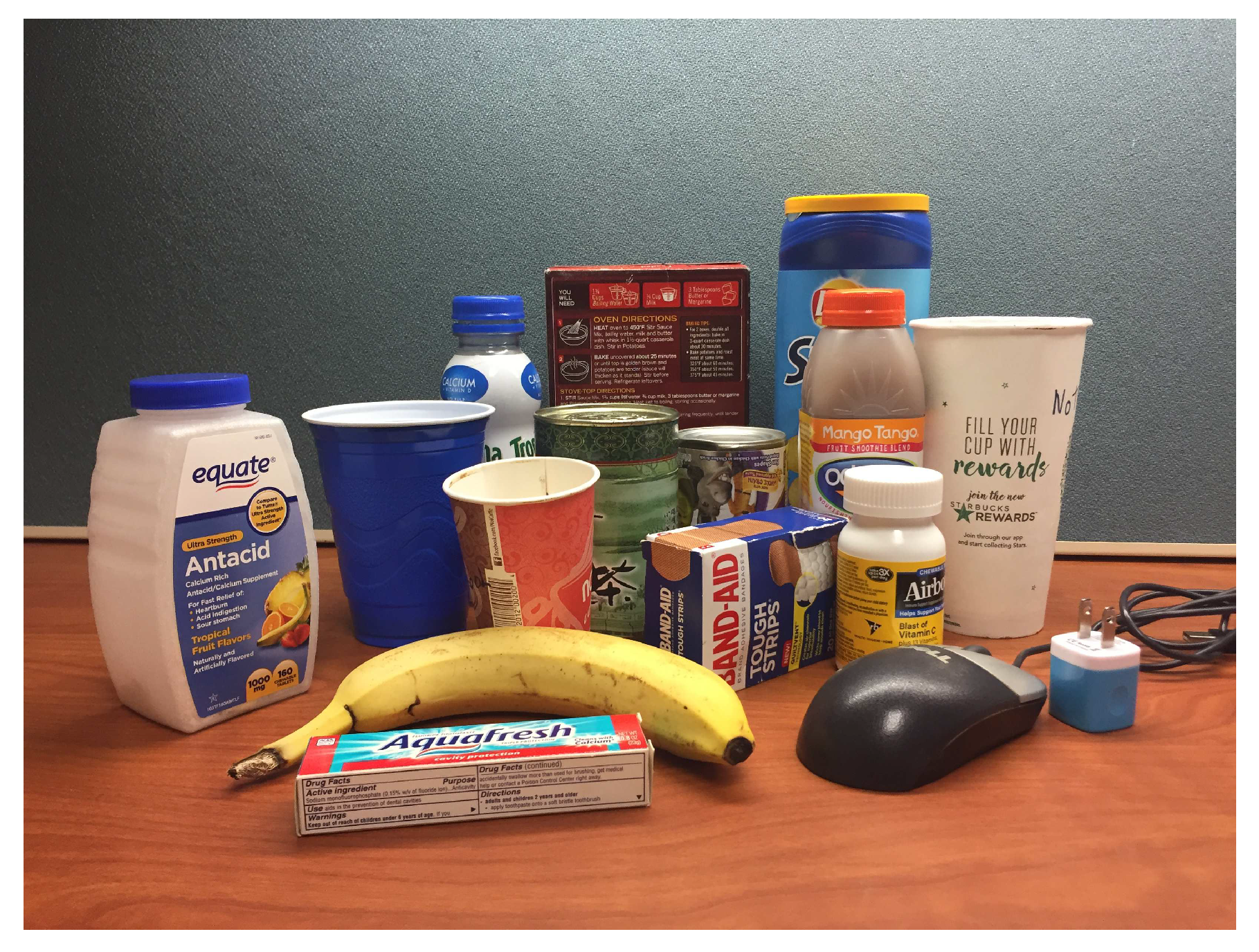Figure 15 displays all the objects were used in the experiments and

Table 2. Single object experiment results. Four attempts for each object are performed. “L” indicates the large size and “S” indicates small-size objects.

Object	% Succ.	Object	% Succ.
Toothpaste Box	100	L Box	100
S Blue Box	75	L Paper Cup	100
Banana	100	L Plastic Cup	100
S Paper Cup	75	Green Cylinder	100
Apple Charger	75	L Pill Container	100
Tropicana Bottle	100	Chips Container	75
S Pill Container	100	Smoothie Bottle	100
Mouse	50	Fruit Can	100
Average: 90.62%

shows the obtained results in the single object experiment.

According to the provided rates, 90% of the robot attempts were successful for the entire set where 11 objects were grasped successfully in all 4 iterations, 4 objects failed to be grasped successfully in 1 out of 4 iterations, while one object (mouse) had 2 successful and 2 unsuccessful attempts. In the unsuccessful attempts, the inappropriate orientation of the gripper during approaching moment is observed as the main reason of failure (4 out of 6) preventing the fingers from forming force-closure on the desired contact regions. Basically, this relates performance of plane extraction from the detected contact regions. Observations during the experiments illustrate high sensitivity of the plane retrieval step to existence of unreliable data in the case of curved shape objects. For instance, in grasping the toothpaste box, although estimated normal direction (${\overrightarrow{V}}_R$) made a $19°$ angle with the expected normal direction (actual normal of the surface), the object was lifted successfully. However, a $9°$ error resulted in failure to grasp the mouse. Impact of force-closure uncertainties on the mouse case is also noticeable. For the other 2 unsuccessful attempts in the single object experiment, inaccurate positioning of the gripper was the main reason for the failure. For grasping the apple charger, gripper could not contact the planned regions, due to noisy values retrieved from low number of pixels on the object edges.

Multi-object experiments are conducted to demonstrate the algorithm overall performance in a more complex environment. In each scene, a variety of objects are placed on the table and the robot approaches the object of interest in each attempt. Measuring the reliability and quality of candidate grasps is not in the scope of this paper. Hence, the order of grasping objects is manually determined such that:

(i)

the objects which are not blocked by other objects in the view, are attempted first.

(ii)

the objects, pursuant to lifting, result in scattering the other objects are attempted last. Therefore, the user chooses one of the candidate grasps and robot attempts the target object unless there are no feasible grasps in the image. This experiment includes 6 different scenes, two scenes with box shaped objects, two scenes with cylinder-shaped objects and two scenes with a variety of shapes.

Table 3. Multi-object experiment results. The success rate implies number of objects grasped successfully out of total number of objects in the scene.

Scene No.	Objects	Grasped Objects	Total Attempts
1	Boxes	4 out of 4	4
2	Boxes	5 out of 5	5
3	Cylinders	4 out of 5	6
4	Cylinders	5 out of 5	6
5	Mix.	5 out of 6	8
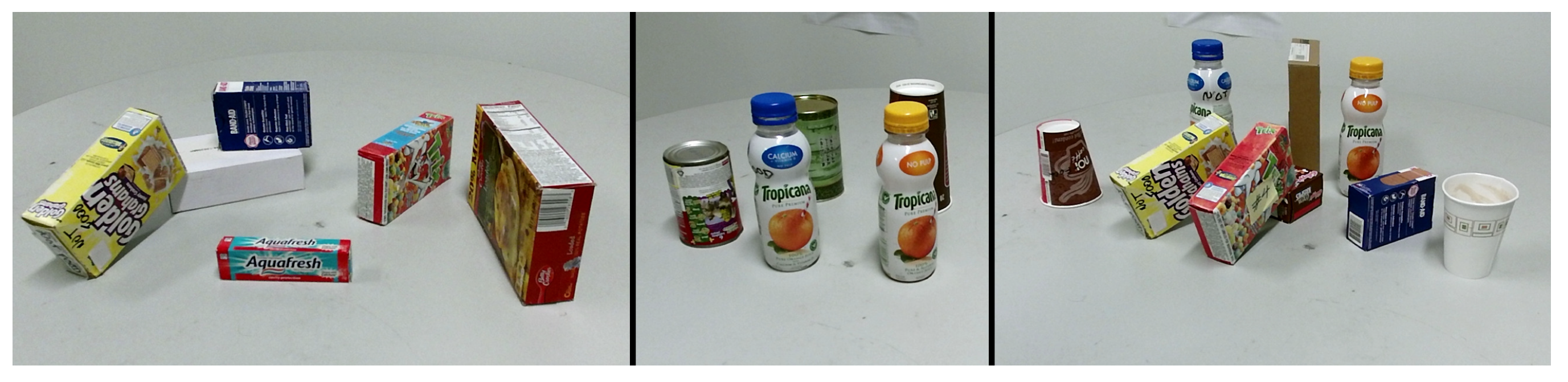
6	Mix.	5 out of 8	8

indicates the obtained results of multi object experiment while Figure 16 demonstrates the setups of three of the scenes.

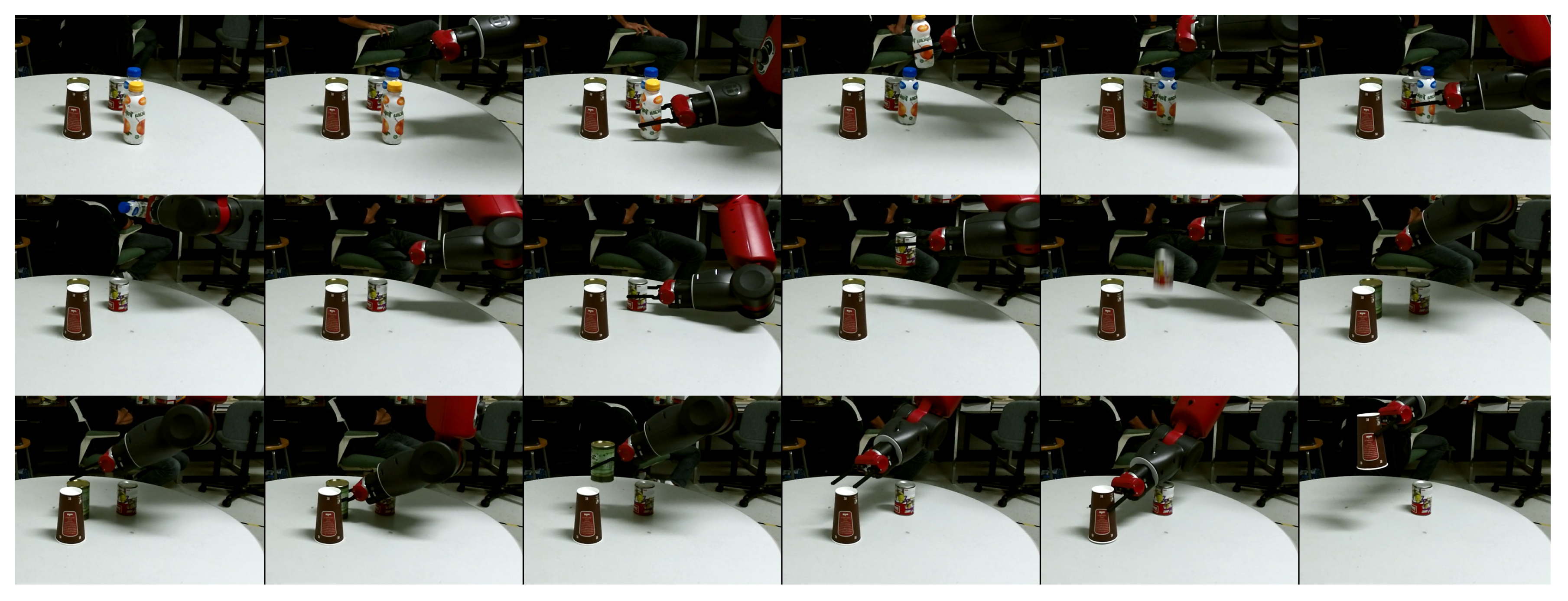
Based on the obtained results, the proposed approach yields a 100% successful rate for box shaped objects, 90% for curved shapes, and 72% for very cluttered scenes with mixed objects. Figure 17 indicates a sequence of images during the grasp execution for the scene #3 in the multi-object experiment. During the grasp execution for scene #3 in (Figure 16) in the multi-object experiment. The robotic arm attempted to grasp the cylinder-shaped objects located on the table. In the first two attempts, orange and blue bottles were successfully grasped, lifted and removed from the scene. Although in the third attempt, the gripper contacted the paste can and elevated it, the object was dropped due to lack of sufficient friction between the fingertips and object surface. Then, the arm approached the remaining objects (green cylinder and large paper cup) and grasped them successfully. In the last attempt, another grasp was planned for the paste can by capturing a new image. This attempt also failed because of inaccurate pose estimation. Finally, the experiment was finished with one extra attempt and with a success rate of 80% (specifically, 4 out of 5).

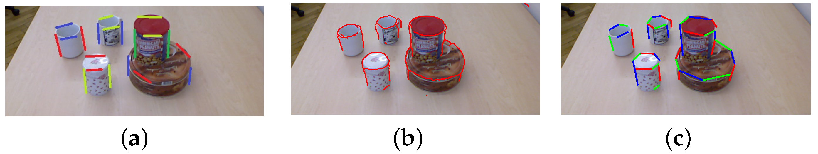
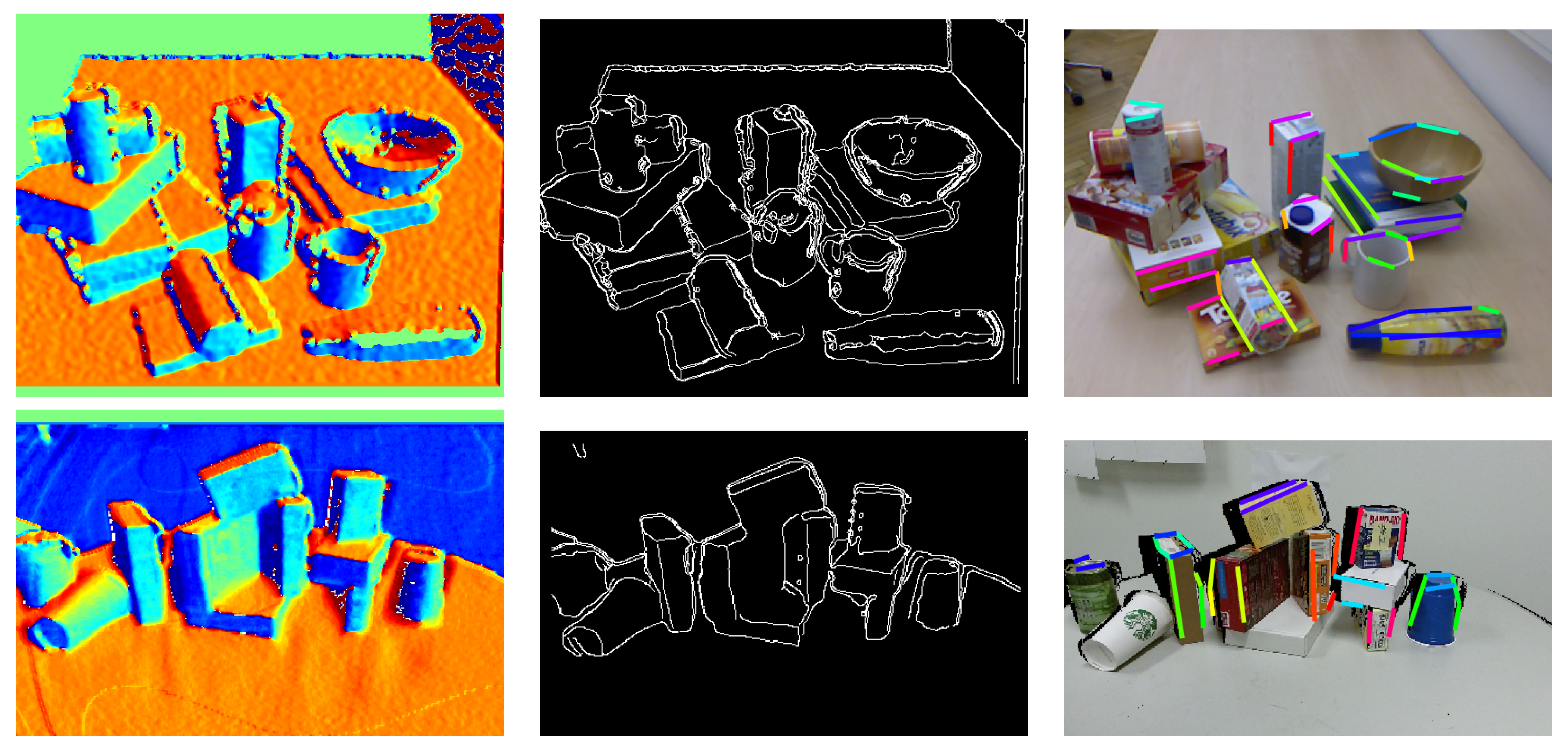
Figure 18 illustrates outcomes of three steps of the algorithm. The left column pictures indicate a color map of depth gradient direction images, the middle column demonstrates detected depth edges before any post-processing, and the last column shows candidate grasps presented by a pair of same color line segments. As discussed in the Implementation Section, 3D coordinates of edge points result in 6D pose of end-effector. Please note that scene in the first row is from OSD dataset and scene in the second row is collected through our experiments. A video of the robot executing grasping tasks can also be found on-line at [42].

6.3. Discussion

According to the implemented approach, we discuss the performance of the approach and failure reasons at different levels, namely 2D contact region detection, 3D grasp extraction, and execution. In the detection phase, the output is a pair of 2D line segments. False positive and false negative pairs are caused by the following reasons: (i) inefficiency of edge detection, (ii) incorrect identification of edge type feature(DD/CD), and (iii) incorrect identification of wrench direction feature ($\pm ,+,-,0$). The aforementioned errors are caused by measurement noise and appearance of artifacts in the data. However, objective modification based on specific datasets can yield performance improvement. Please note that if we perform detections on a synthetic dataset without adding noise, these reasons do not affect the output.

Since the user selects a desired Tpair, false positive output of detection phase does not impact the grasp attempt in the conducted experiments. As a matter of fact, in the 3D grasp extraction step, the approach provides grasp parameters ($P_G,{\overrightarrow{V}}_R,{\overrightarrow{V}}_C$) based on a true positive pair of contact regions. Overall, the grasp parameter estimation errors can be sourced to the following underlying reasons: (i) inaccurate DD edge pixel placement(foreground/background), (ii) unreliable data for low pixel density objects, and (iii) noise in the captured data. Since we derive contact regions instead of contact points, deviation of $P_G$ in certain directions is negligible unless the finger collides with an undesired surface while approaching the object. Width of the gripping area with respect to the target surface determines limits for this deviation. Furthermore, error in estimation of ${\overrightarrow{V}}_R$ also results in force exertion on improper regions and consequently results in an unsuccessful grasp. Sensitivity of a grasp to this parameter depends on the surface geometry and finger kinematics. Compliant fingers show high flexibility to the estimated plane error, while firm wide fingertips do not tolerate the error. Uncertainties and assumptions regarding the friction coefficient, robot calibration, and camera calibration errors are among the factors impacting the performance of the execution step.

Obtained results also indicate that the efficiency of the proposed approach (in terms of average detection time needed per pair of graspable edges) increases as the scene becomes more cluttered. However, as expected, the total time to process a scene correlates well with the complexity of the scene. Addressing how exactly the performance of these pixel-wise techniques, such as edge detection and morphology operations, affect the efficiency of our approach is complex. Output quality and setting of these methods strongly depend on characteristics of the image view and scene. Therefore, we only analyze edge length effects and avoid detailing other effective parameters. In fact, an edge appearing longer in a 2D image is composed of a greater number of pixels. Thus, it has a smaller chance of being missed in the detection step. In addition, since there is uncertainty in the measured data, a longer 2D edge signifies more reliable information in the grasp extraction step. On the other hand, appearance of an edge in the image relies on the distance and orientation of the object regarding the camera view. Thus, depth pixel density of an object in 2D image affects the detection performance and reliability of its corresponding grasp.

7. Conclusions

We have proposed an approach to grasp novel objects from a scene containing multiple objects in an uncontrived setting. Our algorithm estimates reliable regions on the contours (formed by a set of depth edges) to contact the object based on geometric features extracted from a captured single view depth map. The proposed algorithm leads to a force-closure grasp. Real-world experiments demonstrate the ability of the proposed method to successfully grasp a variety of objects of different shapes, sizes, and colors. Future work will focus on four directions: (1) illustrating implementation of approach for a general multi-fingered gripper (2) extracting more geometric features from the available data to control the uncertainties, (3) employing efficient techniques to reduce the noise effects and, (4) equipping the approach with a process to evaluate the grasp quality and reliability.