Fault Diagnosis for UAV Blades Using Artificial Neural Network

Abstract

In recent years, unmanned aerial vehicles (UAVs) have been used in several fields including, for example, archaeology, cargo transport, conservation, healthcare, filmmaking, hobbies and recreational use. UAVs are aircraft characterized by the absence of a human pilot on board. The extensive use of these devices has highlighted maintenance problems with regard to the propellers, which represent the source of propulsion of the aircraft. A defect in the propellers of a drone can cause the aircraft to fall to the ground and its consequent destruction, and it also constitutes a safety problem for objects and people that are in the range of action of the aircraft. In this study, the measurements of the noise emitted by a UAV were used to build a classification model to detect unbalanced blades in a UAV propeller. To simulate the fault condition, two strips of paper tape were applied to the upper surface of a blade. The paper tape created a substantial modification of the aerodynamics of the blade, and this modification characterized the noise produced by the blade in its rotation. Then, a model based on artificial neural network algorithms was built to detect unbalanced blades in a UAV propeller. This model showed high accuracy (0.9763), indicating a high number of correct detections and suggests the adoption of this tool to verify the operating conditions of a UAV. The test must be performed indoors; from the measurements of the noise produced by the UAV it is possible to identify an imbalance in the propeller blade.

1. Introduction

Unmanned aerial vehicles (UAVs) are aircraft characterized by the absence of a human pilot on board. The flight of this vehicle is controlled by the computer on board the aircraft, under the remote control of a navigator or pilot on the ground or in another vehicle [1]. Initially UAVs were used exclusively in the military environment, in dull missions (monotonous and long-lasting surveillance and reconnaissance), in dirty missions (dangerous for the safety of the pilots), and in dangerous missions (risky for the life of the pilots) [2]. The enormous potential, the successes achieved in military missions, and the progress made in the field of micro and nano-technologies have prompted various industries and universities to develop numerous UAS (unmanned aerial systems) that are increasingly modern and reliable, and able to be used in a wide range of civil and military applications [3]. Nowadays, they represent the future of modern aeronautics.

UAVs represent a valuable tool for new hi-tech professions: high-resolution photographic take-over and three-dimensional reconstructions of territory are examples of the use of these technologies. Also, the use of UAVs is essential for professionals in carrying out their existing jobs. Engineers, journalists, videographers, farmers, first aid workers, law enforcement and the military are discovering how to use this new technology to improve their work activities [4].

Usually, in the civil field, very simple means of control and relatively inexpensive multi-copters are used. In fact, multi-copters are small air vehicles with more propellers, usually from three to eight. Four-propeller configurations are very common due to their simplicity and low cost, and are excellent for flying indoors or flying over low-level public spaces [5]. They are mechanically simpler than a helicopter, although less efficient. In small dimensions, mechanical simplicity fully compensates for the lower efficiency.

Faults are very expensive for every industrial plant because they impose a repair of the machine, and also generate stop periods in the entire manufacturing process, with consequent loss of revenue. To overcome these problems, companies resort to predictive maintenance, which is a type of preventive maintenance that is carried out following the identification of one or more parameters that are measured and extrapolated using appropriate mathematical models in order to identify the time remaining before the failure. This method requires effort; it is necessary to plan the interventions at regular intervals and to pay a specialized worker who carries out the adjustments. However, by constantly monitoring the status of the machine, it is possible to detect faults and plan maintenance as needed, avoiding unnecessary checks.

The use of fault diagnosis (FD) techniques is becoming increasingly important in order to ensure high levels of safety and reliability in automated systems and autonomous or remotely controlled systems [6]. In fact, in recent years the international scientific community has made considerable efforts to develop systematic approaches to FD in various systems. The main purpose of an FD algorithm is to monitor a system during its operation in order to detect the occurrence of faults (fault detection), locate faults (fault isolation) and determine their temporal evolution (fault identification). The model-based approach to FD achieves these objectives by comparing the actual behavior of the monitored system with that predicted by a mathematical model [7].

Typically, the output of a system for the FD is a set of variables sensitive to the occurrence of faults (residuals), modified by a signature when the system is subject to failure (fault signature). Thus, the information contained in the fault signature is extracted and processed to detect, isolate and identify faults [8]. In the literature, there are numerous references to many existing FD techniques and the most recent developments, which are not only in the aeronautical field. Fault detection algorithms can be divided into three groups: model-based approaches, expert systems and data-driven solutions based on signal processing [9,10,11,12,13,14,15,16,17,18,19,20,21,22,23,24,25,26].

Among these, those based on machine learning algorithms are gaining more and moreinterest. These techniques have been used in various areas of fault diagnosis. Guo et al. proposed a hybrid feature model and deep learning-based fault diagnosis for UAV sensors. The model uses the residual signals of different sensor faults, including a global positioning system (GPS), inertial measurement unit (IMU), and air data system (ADS) [27]. Bondyra et al. presented a three-stage algorithm based on signal processing and machine learning to identify the occurrence of a rotor fault and detect its scale and type. The algorithm uses the measurements of acceleration from the onboard IMU sensor to detect the fault. Indeed, unbalanced rotating parts are sources of vibrations in mechanical systems. To obtain a characteristic signature of the faulty state, the acceleration signal is first stored in a cyclic buffer and then processed by simple feature extraction algorithms [28]. Marichal et al. studied incipient defects in spur gears in a single propeller system of a small-sized unmanned helicopter. Different vibration signals were measured, and their temporal frequency characteristics were taken as inputs to the diagnostic system based on neural networks, fuzzy systems and genetic algorithms [29]. Xie et al. diagnosed the unmanned helicopter rotor’s unbalance fault using a method based on the particle swarm optimization algorithm and generalized regression neural network (PSO-GRNN). The authors used the average mean square error obtained from cross-validation as the fitness function of the particle swarm. Then, the optimal GRNN smooth factor is gained by adopting the particle swarm optimization algorithm. Finally, an optimal model for fault diagnosis is obtained. [30]. Li et al. used a model based on a deep Gaussian-Bernoulli Boltzmann machine (GDBM) exploiting the statistical characteristics of the vibration measurements of rotating machines. The signals of the vibration sensors collected by rotating mechanical systems are represented in the time, frequency and time frequency domains, each of which is then used to produce a set of statistical characteristics [31].

The imperfections of the blades can cause undesirable effects. In recent years, several studies have been carried out on this topic in the field of wind turbines. Joshuva et al. developed a model that is able to predict the various blade faults that occur in the wind turbine blade while the turbine is in operation—vibration signals are used to do this. This algorithm is applicable for real-time analysis, and furthermore, the monitoring can be done on a portable device with less computation time. The authors’ goal was to classify whether the blades are in good condition or in a fault state. In the latter case, the objective is to isolate the condition of the fault. Thus, a decision tree was used for feature selection, then a J48 decision tree-based classifier was used to detect the faults [32]. Gong et al. presented a simulated investigation of wind turbine unbalance faults by creating a pitch angle twist and weight loading on the blade and simulated this by using continuous wavelet transform. Three different scenarios were simulated: normal operating conditions, blade imbalance, and aerodynamic asymmetry. The blade imbalance was added by scaling the mass density of one blade, which created an uneven distribution of mass with respect to the rotor. The aerodynamic asymmetry was added by adjusting the pitch of one blade, which created an uneven torque across the rotor [33]. Kusiak et al. proposed a data-driven approach for monitoring blade pitch faults in wind turbines using SCADA data. This study simulated the blade angle asymmetry and five classifiers were used to identify the best predictor for a data set: bagging, neural network (NN), K-nearest neighbor, and genetic programming (GP). Among these, GP provided the best results and the solutions obtained could be easily interpreted [34]. Laouti et al. presented a study on fault detection in wind turbines using support vector machines (SVM). In this work, SVM were used for fault detection and isolation in a variable speed horizontal-axis wind turbine composed of three blades and a full converter. The SVM algorithms provide a robust method and are based on structural risk minimization, which enhances generalization and accounts for process non linearity by using flexible kernels, such as radial basis function [35]. Godwin et al. built a classifier to detect wind turbine pitch faults through SCADA data analysis and the RIPPER algorithm. The RIPPER algorithm [36], is an extension of the IREP algorithm [37], utilizing the reduced error pruning (REP) used in decision tree algorithms. The procedure proposed by Godwin et al. achieved a 87.05% classification accuracy in pitch angle faults [38].

A defect in the propellers of the drone can cause a possible fall to the ground of the aircraft with consequent destruction, and can also create a safety problem for objects and people who are in the range of action of the aircraft. Therefore, some researchers have tried to analyze the problem from different points of view. Baskaya et al. used a supervised classification method, SVM (support vector machines) to classify the defective and nominal flight conditions of a UAV. The selected features were the gyroscope and accelerometer measurements, and the error considered was the loss of effectiveness in the control surfaces of the drone [39]. Pourpanah et al. developed a monitoring system to identify eventual faults of UAV motors and propellers. The Motor current signature analysis (MCSA) approach was applied to analyze the stator current signals for different conditions. Fuzzy adaptive resonance neural network was used to recognize when the system was operating in a normal or faulty condition. Also, the vibration signature analysis (VSA) technique was applied to check the UAV propellers. A Q-learning-based Fuzzy ARTMAP NN was employed to extract statistical features. Finally, to select an optimal subset of features in an off-line manner, the genetic algorithm (GA) was applied in order to reduce computational time [40]. Rangel-Magdaleno et al. proposed a method for detecting the unbalanced blade on a UAV by analyzing the emitted sound. Sound signals were acquired during take-off and hovering, then analyzed using DWT decomposition and Fourier transform. The tests were performed using a balanced blade and an artificially unbalanced blade. The results show that the proposed methodology can distinguish between a balanced and unbalanced blade [41]. Pechan et al. conducted experimental acoustic measurements to evaluate the noise emitted by UAV helices with surface imperfections. Various propellers with different blade imperfections have been acoustically tested. The measured sound pressure level tells us that some surface imperfections do not affect the noise produced, while other types of imperfections may slightly increase the noise level emitted at low rotation speeds or may slightly reduce the noise level produced at high speeds rotation [42].

In this study the data obtained from the acoustic measurements of the noise produced by a UAV were used to train a model based on neural networks in order to create a system capable of detecting an imbalance in a quadrotor’s propeller. Machine learning techniques are particularly efficient for the early recognition of operating anomalies. in. In practice, the system can be used in the check procedure of the operating conditions of the UAV, which is carried out before each flight. This methodology can be particularly advantageous in that any anomaly will be highlighted before it causes an accident. In the case of an aircraft, an accident in flight not only causes total damage to the device in most cases, but it can also cause damage to people and objects in the vicinity. The choice of algorithm was based on the following considerations. Neural networks are widely used in pattern recognition because of their ability to generalize and to respond to unexpected inputs. In the training phase, the network learns to recognize various specific models based on the labels associated with them. In the execution phase, the network associates to each model identifies the relative label and if it identifies a pattern not associated with a label, then the label less different from the input is selected. In this way, the model based on neural networks shows its capacity for generalization.

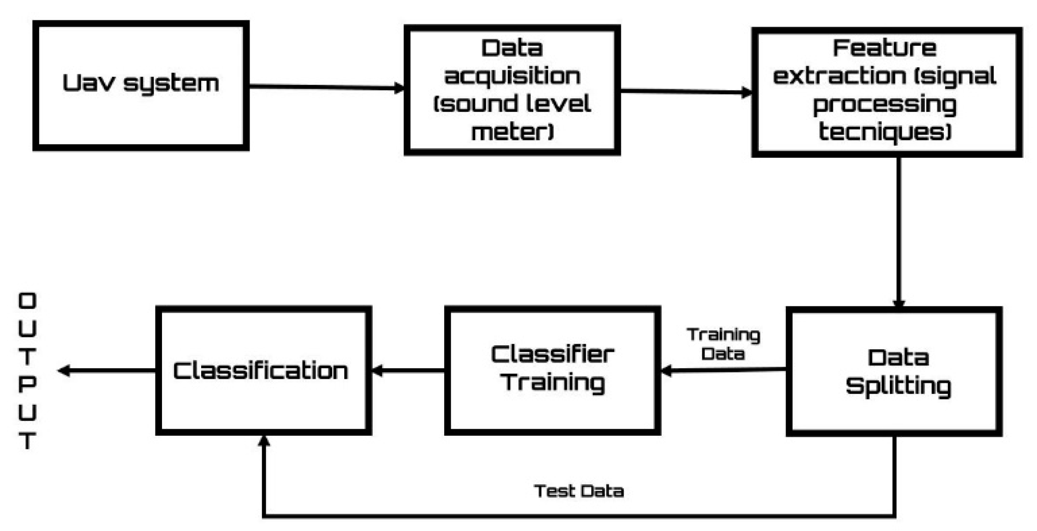
2. Materials and Methods

The objective of this study is to develop a procedure for checking the operating conditions of a UAV. This procedure could be followed before using the UAV for a flight, a procedure like that performed by pilots of airliners before take-off (preflight checklist). The procedure involves a test to be carried out in indoor environments; the noise produced by the UAV is measured and eventually an unbalance in the propeller blade can be identified. To do this, we used the measurements of the noise produced by the UAV in three operating conditions: balanced blade, unbalanced blade 1, and unbalanced blade 2. These measures were processed to extract features that were later used to train and test a classifier based on an artificial neural network. The flow chart of the study procedure is shown in Figure 1.

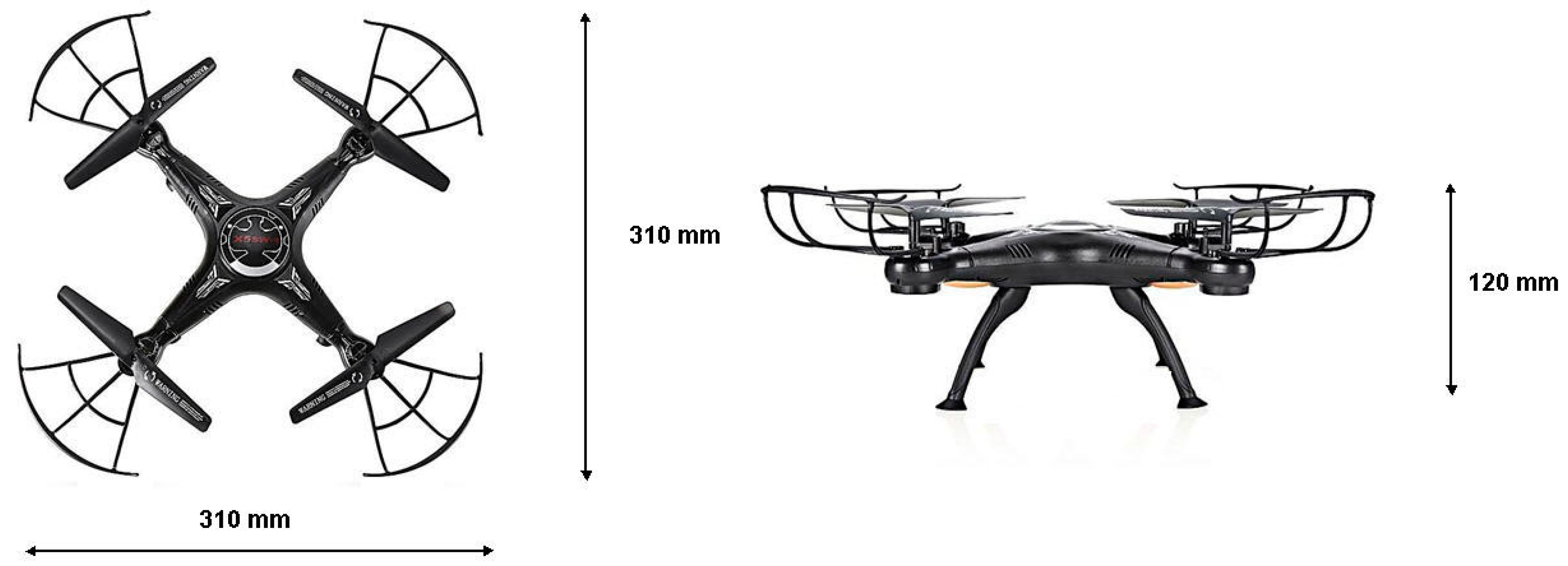
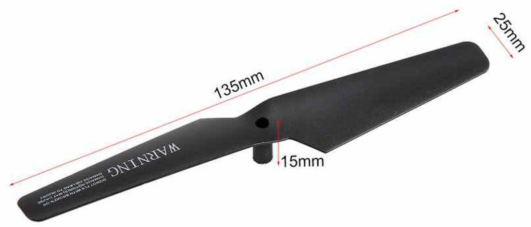
2.1. Unmanned Aerial Vehicle System

The UAV under analysis is a radio-controlled quadcopter equipped with a high-quality ABS hull (Figure 1). The device has four feet, which provide support in landing operations. The drone is equipped with a remote control with a frequency of 2.4 GHz with a control distance of 80 m. A 6-axis gyroscope allows for strong balance in the air and precise hovering, even when there is a light wind due to the four-axis structure. In Figure 2 the drone’s dimensions are specified.

The force necessary for the propulsion of a UAV (thrust) is obtained by accelerating a mass of fluid in the opposite direction to the direction of motion in order to vary the momentum of the air flow. The operation is based on Bernoulli’s principle and on Newton’s third principle of dynamics, whereby a body that exerts a force on another body (the propeller on the air mass) receives an equal and opposite reaction force (air mass on the propeller), which causes the propeller advancement. In the analyzed drone (quadcopter), two propellers move clockwise while the other two propellers move counterclockwise. The direction of rotation alternates in the arrangement of the four propellers.

The propeller therefore represents the fundamental element that determines the performance of the device as well as for the intensity of the noise produced during operation. A propeller is basically made up of two parts: the hub and the blades. The hub is the central part, usually perforated to be inserted in the crankshaft. It has an ogival shape to minimize the resistance to advancement (vertical). The blades are the elements that allow the actual generation of the traction force. The analyzed drone has propellers with 2 blades as shown in Figure 3.

A propeller is characterized by two sizes: the diameter and the pitch. The diameter is the tip-to-tip distance of the 2 blades and constitutes the work area of the propeller (in our case it is 135 mm, Figure 3). It corresponds to the diameter of the disc that circumscribes the propeller. The pitch is defined as the distance that the propeller travels in ideal conditions during a complete rotation. The pitch represents the height of the air column that will be moved during the complete rotation. The pitch is the incidence of the wing profile or the inclination of the propeller with respect to the support pin.

The shape of the propeller plays an important role in the performance of the drone. The terminal part (tip) induces different effects, as it is there that the air flow is more turbulent. Propellers can be distinguished by their tip shape, which include the bull nose (BN), hybrid BN (HBN), and pointy nose. The thrust generated by these blades is different, the HBN generates a greater thrust than BN, which in turn, generates more thrust than the pointed nose.

In general, the noise produced by an aerial vehicle is composed of the following elements: engine noise, propeller noise, airframe noise and aircraft system noise. Due to the size of the UAVs that we are analyzing, we can consider the last two components negligible [43]. Moreover, since we want to identify defects in the propellers of a quadcopter, we will only analyze this element in detail. The noise generated by the propellers is composed of two components: rotational and that due to the vortex. Rotational noise is periodic, it represents the sound produced by the rotation of the blades and it is identified with discrete frequencies given by the product of the number of blades multiplied by the rotation frequency. The noise due to the vortex is created on the end of the blade. This is a modulated broadband noise produced by the unstable pressure field associated with the vortices scattered from the rear edge and blade tips, as well as some of the noise sources associated with the effects of turbulence in the air flow [44].

As we have already mentioned, the purpose of this study is to identify an imbalance on one of the four blades of the UAV. To simulate the unbalanced condition, two strips of paper tape were applied to the upper surface of a blade. The paper tape denotes a substantial modification of the aerodynamics of the blade, and this modification characterizes the noise produced by the blade in its rotation. Figure 4 shows three different blade configurations: balanced blade, unbalanced blade with one strip of paper tape, and unbalanced blade with two strip of paper tape.

The paper tape creates a surface with a friction that is substantially different from that provided by the blade wing profile. Thus, the lift of the propeller is also modified.

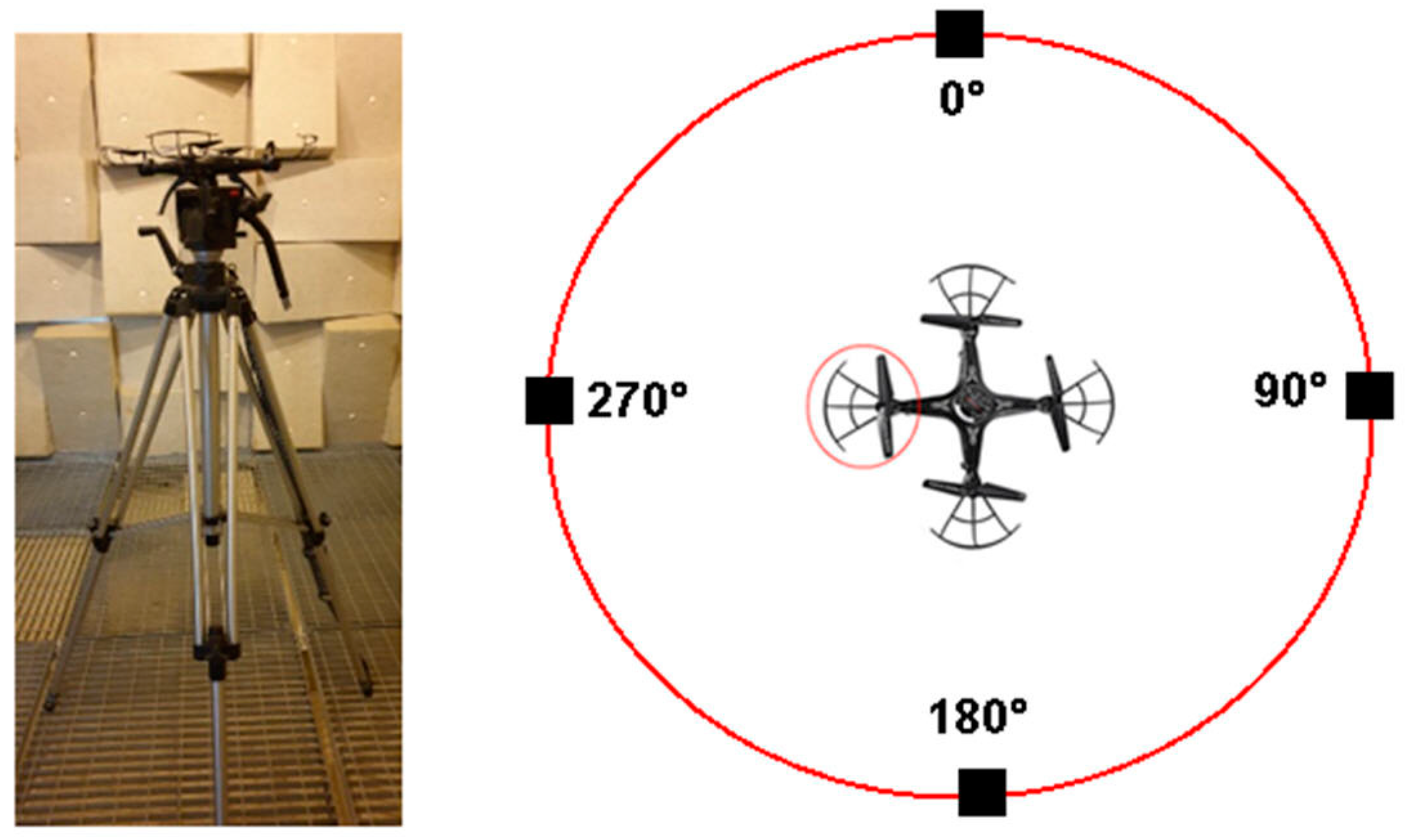
2.2. Data Acquisition

For each of the three configurations shown in Figure 4, acoustic measurements were taken to characterize the UAV blade sound emissions. Measurements were carried out in an anechoic chamber (4.40 m × 4.40 m × 4.50 m), covered by absorptive fiberglass wedges. This is a laboratory environment structured to reduce as much as possible the reflection of signals on the walls. The cut-off frequency of the chamber is 100 Hz.

The choice to use the acoustic measurements to identify an operating fault is dictated by the fact that the current methods of fault diagnosis for rotating machinery require the contact of the sensor with the moving object such as vibration detection, detection of the temperature and so on. In the case of rotating blades, this type of measurement may present problems.

To simulate flight conditions, the UAV was anchored to a tripod using plastic clamps and placed in the center of the anechoic chamber (Figure 5). The choice to position the UAV on the tripod was dictated by the need to create a fixed source-receiver system, in order to reduce the positioning error and obtain good signal acquisition. The acoustic measurements were performed using the following instrumentation [45]:

• Solo 01dB integrating sound level meter model of “Class 1”
• Class 1 calibrator to IEC 60942:2003
• Tripod

The instruments used comply with the requirements of the UNI EN ISO 3745:2012 standard [46]; the sound level meter has been configured for the acquisition of the linear sound pressure level, weighted “Lin”, with a fast time weighting. Fast time weighing is typically the selected weighting for most noise measurements. It is about 8 times quicker than slow weighting and corresponds to roughly 125 milliseconds. One-third octave spectral frequencies were also measured with a sampling frequency of 51.2 kHz.

The sound level meter was placed on a tripod at the same height as the UAV. The measurements were made in 4 positions placed at angles offset by 90 degrees on the circumference with a 1.2 m radius, in the center of which the UAV was placed [46]. Three measurement sessions were performed, corresponding to the three operating conditions of the blade (balanced, unbalanced with one strip of paper tape, and unbalanced with two strips of paper tape.)

For each measurement the UAV was brought to the maximum available speed and it was maintained at this condition for about 10s.

2.3. Feature Extraction

The measurements collected were subjected to post processing using signal processing technique (frequency analysis). The noise produced by the UAV is not composed of pure tones, which are characterized by a signal of a specific frequency, but of a complex type, that is, they are characterized by a wide range of frequencies with different levels. In such circumstances, it is essential to carry out the frequency analysis of the sounds through the quantification of the energy content in the different bands, that is, in specific frequency intervals. Performing frequency analysis means starting from a representation of sound in the time domain, that is, from the waveform, and arriving at defining the spectrum. The spectrum is a graphical representation on a Cartesian diagram that presents the frequencies on the abscissa and a magnitude representative of the amplitude of the sound on the ordinate.

A method for performing frequency analysis of stationary signals involves the use of a “bank” of band-pass filters (such as octave filters), in a series of devices each of which only allows the passage of a given range of frequencies, excluding the sound components at higher and lower frequencies. With a sound meter level at the output of each filter, it is possible to measure the level that competes with the particular frequency range In this phase, the equivalent levels of linear sound pressure, weighted “Lin” were extracted for the 1/3 octave bands, at intervals equal to 125 ms (equal to the integration constant).

2.4. Data Splitting

One of the key problems that must be resolved when working on any machine learning model is the validation of the model, that is, verification of the classification capacity in the case in which input data never seen by the network are used. One of the simplest and most widespread techniques to avoid overfitting (the model adapts to the observed data because it has an excessive number of parameters with respect to the number of observations) is to divide the entire data set into two sub-sets: the training set and test set. The training set is the data used to train the model. The test set is the data set that was not seen by the model so far; that is, the data points are not used in the construction of the model. We can think of the test dataset as the dataset that the model will probably see in the future. Thus, the precision we see on the test data set is probably the accuracy of the model on the future data set. In general, in algorithms based on artificial neural networks, the splitting is done by randomly selecting rows to reduce the bias.

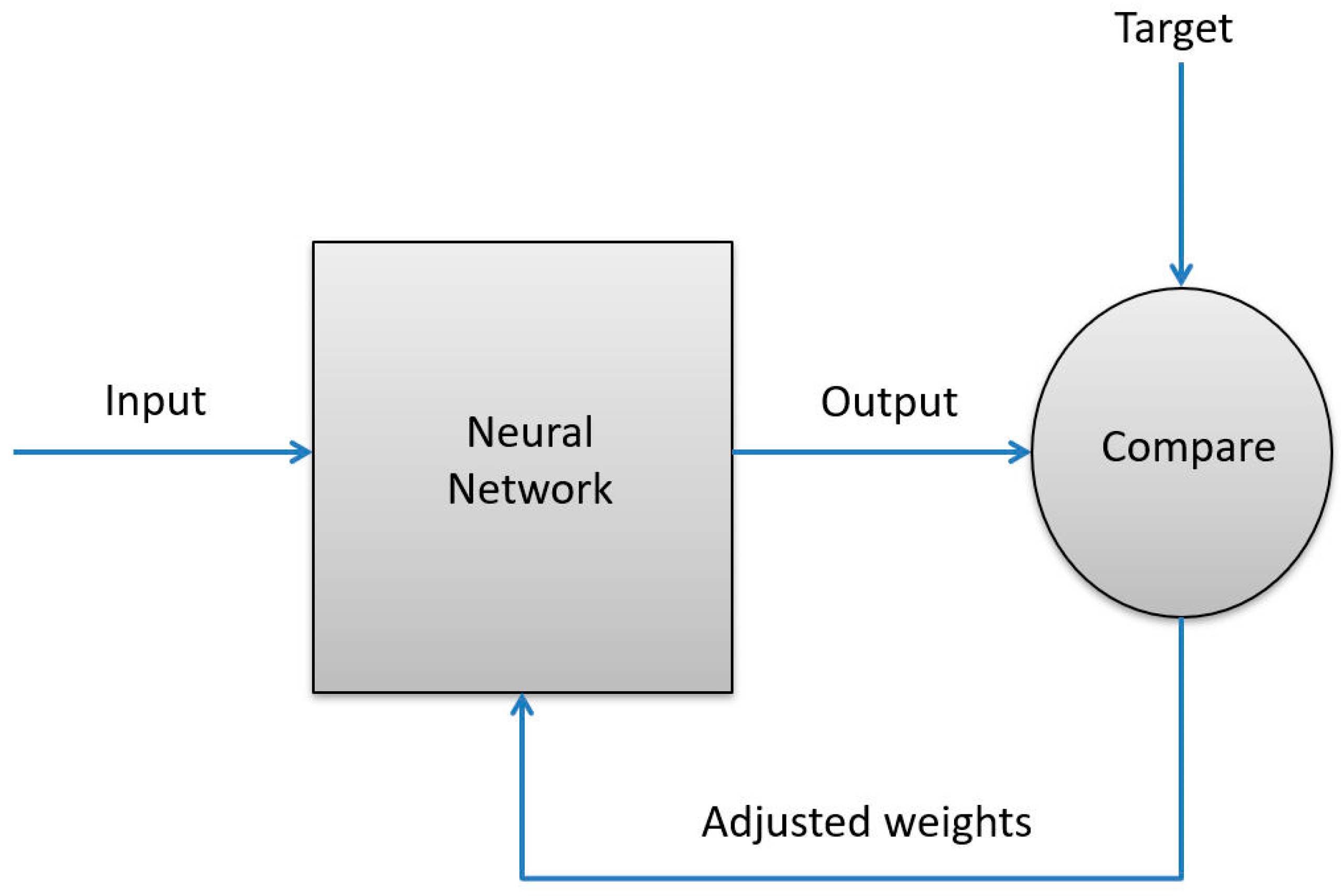
2.5. Classifier Training

Subsequently, the measurements were used to implement a model based on neural networks for the automatic recognition of a UAV blade fault.

Artificial neural networks are information processing systems that try to simulate the functioning of biological nervous systems within an information system. Biological nervous systems are made up of many nerve cells or neurons connected to each other in a complex network. Each neuron is connected on average with tens of thousands of other neurons. Hence, there are hundreds of billions of connections. Intelligent behavior emerges from the numerous interactions between interconnected units; each connection has a weight associated with it that can be tuned based on experience, making neural nets adaptive to inputs and capable of learning.

A neural network is a computational system that was initially inspired by the way the brain processes a learning task. The term artificial neuron, identifies a unit with a central body and input and output terminations. The neurons are organized to form a structure with parallelism, that is, the parts that constitute it do not work in cascade but independently of each other; this makes the network robust. The connections are characterized by parameters called weights. Intelligent behavior emerges from the numerous interactions between the interconnected units.

Each neuron performs a very simple operation that consists in activating if the total amount of signal it receives exceeds a certain activation threshold. If a neuron becomes active, it emits a signal that is transmitted along the communication channels to the other units to which it is connected. The following equation shows how the neuron transforms the input x and returns a weighted output y:

$$y={\displaystyle \sum }_i{w}_i\ast x_i$$

(1)

The vector w therefore contains the weights that can be adjusted based on the experience that the network acquires in the training phase. The easiest way to get the weight vector w is to start with a random vector and then iteratively apply the update rule. This procedure can be repeated until the error committed falls below a certain threshold. The following equation shows a perceptron weight update rule:

$$w_i=w_i+\mu \left(y-f \left(x,w\right)\right) x_i$$

(2)

Here:

• x_i is the input
• y is the output
• µ is the learning rate
• f(x,w) is the current model prediction

By defining the loss function as follows:

$$E\left(y, f \left(x,w\right)\right)=\frac{1}{2} {\left(y-f \left(x,w\right)\right)}^2$$

(3)

it is possible to rewrite the perceptron weight update rule as follows:

$$w_i=w_i+\mu \frac{\partial E\left(w\right)}{\partial w_i}$$

(4)

The developed recognition model was based on a feed-forward artificial multilayer neural network, with 1 hidden layer and 3 output classes representing the three operating conditions. The learning paradigm used is supervised. During the training phase, 70% of the input data and the known outputs were randomly selected, based on the available data. During this phase, the training data set was submitted to the network for weighing and error minimization. A flow chart of the training phase is shown in Figure 6.

The ‘‘resilient backpropagation” algorithm was applied in the calculation with ‘‘backtracking”. The ‘resilient backpropagation algorithm determines iteratively the weights of a neural network to minimize the error function finding the local minimum. The ‘backtracking technique updates the weight values, reverting the previous iteration and adding a small value to the weight.

2.6. Classification

After the training phase, the network undergoes testing phases, with the addition of a set of data each containing 30% of the unused data. In this phase we used the test set to verify the functioning of the network. As we already mentioned, this is a set of data that the network has never seen before. This assures us that the network can generalize, that is, it can return a correct classification even when it is faced with new data.

3. Results and Discussion

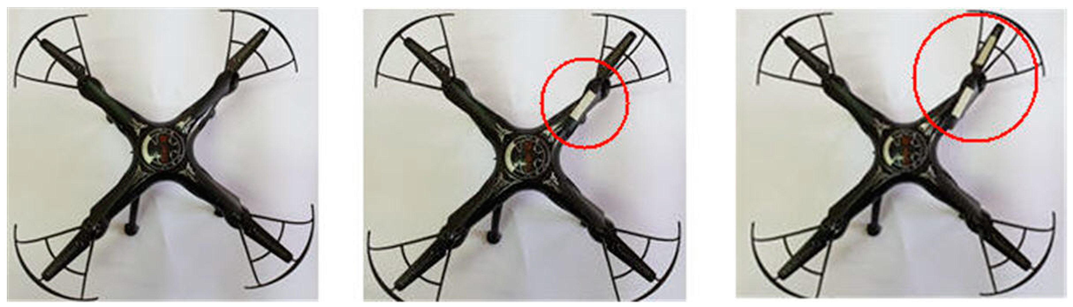
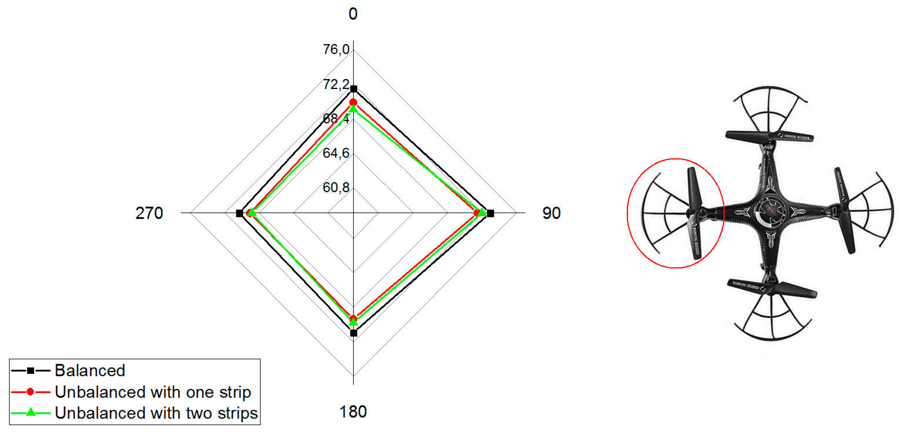
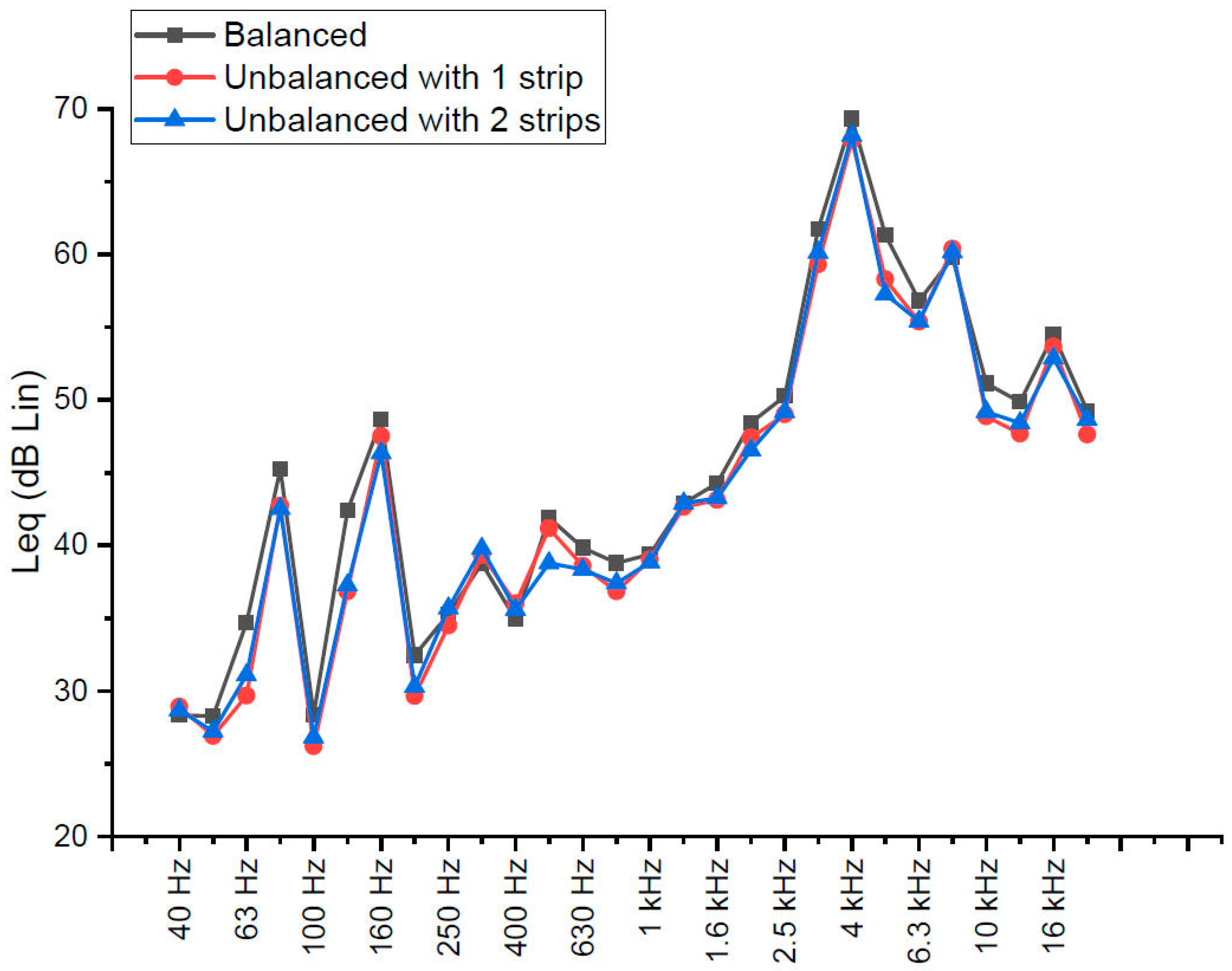
3.1. Acoustic Measurements Analysis

The acoustic measurements were made in 4 positions placed at angles offset by 90 degrees on the circumference with a 1.2 m radius, in the center of which the UAV was placed. Three measurement sessions were performed, corresponding to the three operating conditions of the blade (balanced, unbalanced with one strip of paper tape, and unbalanced with two strips of paper tape). Figure 7 shows the sound pressure level for the three operating conditions at the 4 microphone positions.

Analyzing the diagram shown on the left of Figure 7, it is possible to see that the levels are comparable, both in the 4 microphone positions corresponding to the four propellers, and in the three operating conditions. This suggests that a system based only on the analysis of levels would not be able to identify failures in the UAV blades.

Table 1. Sound pressure level (dB Lin).

Microphone Position	Balanced [dB Lin]	Unbalanced with 1 Strip [dB Lin]	Unbalanced with 2 Strips [dB Lin]
0°	71.7	70.2	69.4
90°	73.1	71.7	72.2
180°	71.2	69.7	70.1
270°	70.6	69.4	69.2

shows the sound pressure level (dB Lin) for the three operating conditions at the 4 positions.

To characterize the operation of the UAV it is necessary to perform a spectral analysis of the noise levels recorded during the measurements. Figure 8, shows the average spectral levels in the 1/3 octave band between 40 Hz and 20 kHz for the three measurement sessions. The spectrum was obtained by averaging the values extracted in the four measurement positions.

Figure 8 shows the noise emitted by the UAV during its operation. Consistent with what was mentioned previously, we can see two discrete low frequency components (80 and 160 Hz). These frequencies correspond to the shaft rate (80 Hz) and to the blade pass frequency (BPF–160 Hz). The BPF is found by multiplying the shaft rate (80 Hz) by the number of rotor blades (2). This tells us that the tonal components identified depends on the rotation speed of the propellers. Therefore, a different engine configuration determines a variation in the BPF due to small variations in the signal supplied to the electric motors. Furthermore, there is a modulated broadband noise between the 2 and 20 kHz frequencies, which has a peak at the frequencies of 4 kHz. This noise is due to unstable aerodynamics caused by the interaction of the air flow with the drone frame, since the blade tips are a short distance from the frame. Another explanation for this may be the interaction of the blades with the wake of the rotor.

3.2. Data Pre-Processing

For the fault recognition analysis, we chose to use the average spectrum in 1/3 octave bands in the 40Hz–20kHz frequency range as the distinguishing feature. In this regard, each observation period was appropriately divided into intervals of 125 ms, for each of which the characteristics just mentioned were extracted. The measurement intervals related to the three operating conditions have been labeled by adding a numerical label (0,1,2).

Table 2. Summary of the data extracted.

	Balanced	Unbalanced with 1 Strip	Unbalanced with 2 Strips
Number of samples	243	287	317
Time constant (ms)	125	125	125
Number of features	31	31	31

shows a summary of the data extracted.

Each feature has a range of values with obvious differences that in some cases can also be marked. If a feature is characterized by much larger numerical values than the others, the information brought by this feature will be dominant, while one of the important criteria for choosing features is the content of information. In addition to the absolute numerical value, the numerical excursion of the feature is also important.

We therefore need to process the data beforehand in order to combine and weigh descriptors to reflect the size or structure of the phenomenon being measured. To do this we carried out a normalization of the data in order to make the descriptors comparable by bringing them to the same standard, reversing the polarity, where necessary and transforming them into pure, dimensionless numbers.

For feature scaling the min-max normalization was used [47]. This technique performs a linear transformation on the original data so as to obtain all the data in scale in the interval (0,1). The formula to get this is:

$$x_{scaled}=\frac{x-x_{min}}{x_{max}-x_{min}}$$

(5)

Min-max normalization maintains the relationships between the values of the original data. The cost of having this limited range is that we end up with smaller standard deviations, which can mask the effect of outliers.

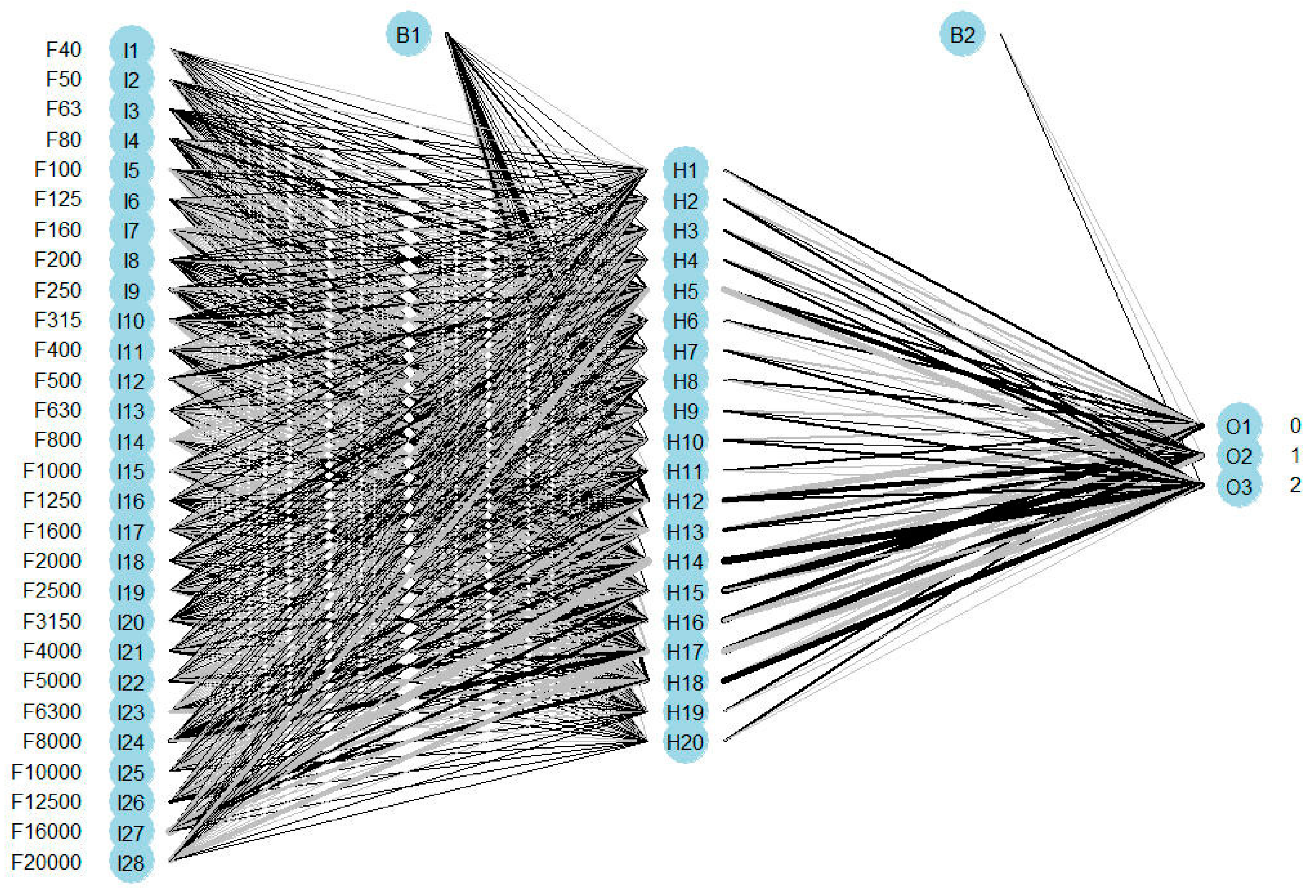
3.3. Neural Network Model

The features extracted in the previous phase were used as input for a model based on artificial neural networks with a single hidden layer architecture and with three outputs related to the variable representing the operating condition.

To measure the performance of a network we must then divide the data into two independent sets, which are called training and test sets, so that we can check how the error varies on both learning and new data introduced later. This is the only way we can find the best hidden number m of units for the network, and we must ensure that the network has enough flexibility, but does not give rise to overfitting. The network to function optimally must have a low error regarding the test data. In our case, we divided the data into two sets: a training set equal to 70% of the data, and a test set equal to the remaining 30% of the data. The subdivision of the observations in both was carried out randomly.

Table 3. Summary of the partitioned data.

	Number of Samples	%
Starting Dataset	847	100
Train data	594	70
Test data	253	30

shows how the data was partitioned.

To allow the network to better approximate the system in question, it was necessary to subject it to a training process. This process consists of controlling the response provided by the network when input values are entered, for which the exact value of the dependent variable is known (training set). For this phase, 70% of the available data were randomly selected. In Figure 9, the neural network architecture with weights and biases highlighted is shown.

Neural network architecture provides only one hidden layer with 20 neurons. Since it is a classification problem with the results falling into the three categories (multi-class classification problem) the SoftMax Activation Function was utilized.

The neural network was trained by adopting the scaled conjugate gradient backpropagation algorithm. This algorithm represents a variant with respect to the basic backpropagation (which regulates the weights in the steepest descent direction), since a search is performed along the conjugate directions, which generally produces a convergence faster than the previous one [48,49].

After the learning phase, the effectiveness of the network was tested on a new set of data, the test set. This set of data was selected from input and output values (30% of those available) never seen before by the network.

Table 4. Confusion matrix (0 = balanced, 1 = unbalanced with 1 strip, and 2 = unbalanced with 2 strips).

		Predicted
		0	1	2
Actual	0	71	1	0
	1	1	83	2
	2	0	2	93

shows a confusion matrix of the results. A confusion matrix is a table that is used to describe the performance of a classification model on a set of data for which the true values are known. The rows correspond to the predicted class and the columns correspond to the true class. The diagonal cells correspond to observations that are correctly classified. The off-diagonal cells correspond to incorrectly classified observations. The number of observations is shown in each cell.

The results obtained from the identification of the network on new observations are excellent. Out of 253 samples tested, only 6 errors occurred with an accuracy = 0.9763.

Table 5. Statistics by class.

	Class 0	Class 1	Class2
Sensitivity	0.9861	0.9651	0.9789
Specificity	0.9945	0.9820	0.9873
Balanced Accuracy	0.9903	0.9736	0.9831

shows some statistics by class.

In Table 5, sensitivity measures the proportion of actual positives that are correctly identified as such. Specificity measures the proportion of actual negatives that are correctly identified as such. Finally, balanced accuracy is calculated as the average of the correct proportion of each class individually.

4. Conclusions

In this study, measurements of the noise emitted by a UAV were used to build a classification model to detect an unbalanced blade in a UAV propeller. To simulate the fault condition, two strips of paper tape were applied to the upper surface of a blade. The paper tape denotes a substantial modification of the aerodynamics of the blade and this modification characterizes the noise produced by the blade in its rotation. In recent years, algorithms based on machine learning have been used to detect faults in machine functioning and control [50,51,52,53,54,55,56,57,58]. First, acoustic measurements were performed in an anechoic chamber and then these were analyzed to characterize the phenomenon [59,60,61,62,63,64,65]. An appropriate number of observations were then extracted, and these data were pre-processed. Subsequently, a model based on artificial neural network algorithms was built to detect unbalanced blades in a UAV propeller. This model showed a high value for accuracy (0.9763), indicating a high number of correct detections and suggests the adoption of this tool for fault diagnosis applications.

The objective of this study was to develop a procedure for checking the operating conditions of a UAV. This procedure could be followed before using the UAV; a procedure like that performed by pilots of airliners before taking-off (preflight checklist). The procedure involves a test to be carried out in indoor environments: the noise produced by the UAV is measured and eventually an unbalance in the propeller blade can be identified. The real system involves the use of an external device. Further research will focus on the use of real damaged blades to better simulate the fault condition. Furthermore, a possible on-board control system will be used to allow real-time fault detection during the flight. Future developments also include methods for extracting features and choosing classifiers based on other machine learning algorithms to improve performance.

References

1. Valavanis, K.P.; Vachtsevanos, G.J. Handbook of Unmanned Aerial Vehicles; Springer: Dordrecht, The Netherlands, 2015; pp. 2993–3009. [Google Scholar]
2. Newcome, L.R. Unmanned Aviation: A Brief History of Unmanned Aerial Vehicles; American Institute of Aeronautics and Astronautics: Reston, VA, USA, 2004. [Google Scholar]
3. Gertler, J. US Unmanned Aerial Systems; Congressional Research Service (Library of Congress): Washington, DC, USA, 2012. [Google Scholar]
4. Rao, B.; Gopi, A.G.; Maione, R. The societal impact of commercial drones. Technol. Soc. 2016, 45, 83–90. [Google Scholar] [CrossRef]
5. Agrawal, K.; Shrivastav, P. Multi-rotors: A revolution in unmanned aerial vehicle. Int. J. Sci. Res. 2015, 4, 1800–1804. [Google Scholar]
6. Gertler, J. Fault Detection and Diagnosis; Springer: London, UK, 2013; pp. 1–7. [Google Scholar]
7. Marzat, J.; Piet-Lahanier, H.; Damongeot, F.; Walter, E. Model-based fault diagnosis for aerospace systems: A survey. Proc. Inst. Mech. Eng. Part G J. Aerosp. Eng. 2012, 226, 1329–1360. [Google Scholar] [CrossRef]
8. Yoon, S.; MacGregor, J.F. Fault diagnosis with multivariate statistical models part I: Using steady state fault signatures. J. Process Control 2001, 11, 387–400. [Google Scholar] [CrossRef]
9. Ding, S.X. Model-Based Fault Diagnosis Techniques: Design Schemes, Algorithms, and Tools; Springer Science & Business Media: Berlin, Germany, 2008. [Google Scholar]
10. Simani, S.; Fantuzzi, C.; Patton, R.J. Model-based fault diagnosis techniques. In Model-Based Fault Diagnosis in Dynamic Systems Using Identification Techniques; Springer: London, UK, 2003; pp. 19–60. [Google Scholar]
11. Glowacz, A. Acoustic based fault diagnosis of three-phase induction motor. Appl. Acoust. 2018, 137, 82–89. [Google Scholar] [CrossRef]
12. Ma, S.; Cai, W.; Liu, W.; Shang, Z.; Liu, G. A Lighted Deep Convolutional Neural Network Based Fault Diagnosis of Rotating Machinery. Sensors 2019, 19, 2381. [Google Scholar] [CrossRef] [PubMed]
13. Toliyat, H.A.; Nandi, S.; Choi, S.; Meshgin-Kelk, H. Electric Machines: Modeling, Condition Monitoring, and Fault Diagnosis; CRC Press: Boca Raton, FL, USA, 2012. [Google Scholar]
14. Chen, J.; Patton, R.J. Robust Model-Based Fault Diagnosis for Dynamic Systems; Springer Science & Business Media: Berlin, Germany, 2012; Volume 3. [Google Scholar]
15. Zedda, M.; Singh, R. Gas turbine engine and sensor fault diagnosis using optimization techniques. J. Propuls. Power 2002, 18, 1019–1025. [Google Scholar] [CrossRef]
16. Nandi, S.; Toliyat, H.A. Fault diagnosis of electrical machines—A review. In Proceedings of the IEEE International Electric Machines and Drives Conference IEMDC’99 Proceedings (Cat. No. 99EX272), Seattle, WA, USA, 9–12 May 1999; pp. 219–221. [Google Scholar]
17. Shen, L.; Tay, F.E.; Qu, L.; Shen, Y. Fault diagnosis using rough sets theory. Comput. Ind. 2000, 43, 61–72. [Google Scholar] [CrossRef]
18. Rai, A.; Upadhyay, S.H. A review on signal processing techniques utilized in the fault diagnosis of rolling element bearings. Tribol. Int. 2016, 96, 289–306. [Google Scholar] [CrossRef]
19. Nandi, S.; Toliyat, H.A.; Li, X. Condition monitoring and fault diagnosis of electrical motors—A review. IEEE Trans. Energy Convers. 2005, 20, 719–729. [Google Scholar] [CrossRef]
20. Kankar, P.K.; Sharma, S.C.; Harsha, S.P. Fault diagnosis of ball bearings using continuous wavelet transform. Appl. Soft Comput. 2011, 11, 2300–2312. [Google Scholar] [CrossRef]
21. Wang, M.H. A novel extension method for transformer fault diagnosis. IEEE Trans. Power Deliv. 2003, 18, 164–169. [Google Scholar] [CrossRef] [Green Version]
22. Edwards, S.; Lees, A.W.; Friswell, M.I. Fault diagnosis of rotating machinery. Shock Vib. Dig. 1998, 30, 4–13. [Google Scholar] [CrossRef]
23. Siddique, A.; Yadava, G.S.; Singh, B. A review of stator fault monitoring techniques of induction motors. IEEE Trans. Energy Convers. 2005, 20, 106–114. [Google Scholar] [CrossRef]
24. Lei, Y.; Lin, J.; Zuo, M.J.; He, Z. Condition monitoring and fault diagnosis of planetary gearboxes: A review. Measurement 2014, 48, 292–305. [Google Scholar] [CrossRef]
25. Gao, Z.; Ding, S.X.; Cecati, C. Real-time fault diagnosis and fault-tolerant control. IEEE Trans. Ind. Electron. 2015, 62, 3752–3756. [Google Scholar] [CrossRef]
26. Fekih, A. Fault diagnosis and fault tolerant control design for aerospace systems: A bibliographical review. In Proceedings of the 2014 American Control Conference, Portland, OR, USA, 4–6 June 2014; pp. 1286–1291. [Google Scholar]
27. Guo, D.; Zhong, M.; Ji, H.; Liu, Y.; Yang, R. A hybrid feature model and deep learning based fault diagnosis for unmanned aerial vehicle sensors. Neurocomputing 2018, 319, 155–163. [Google Scholar] [CrossRef]
28. Bondyra, A.; Gasior, P.; Gardecki, S.; Kasiński, A. Fault diagnosis and condition monitoring of uav rotor using signal processing. In Proceedings of the 2017 Signal Processing: Algorithms, Architectures, Arrangements, and Applications (SPA), Poznan, Poland, 20–22 September 2017; pp. 233–238. [Google Scholar]
29. Marichal, G.; Del Castillo, M.; López, J.; Padrón, I.; Artés, M. An artificial intelligence approach for gears diagnostics in AUVs. Sensors 2016, 16, 529. [Google Scholar] [CrossRef]
30. Xie, X.H.; Xu, L.; Zhou, L.; Tan, Y. GRNN Model for Fault Diagnosis of Unmanned Helicopter Rotor’s Unbalance. In Proceedings of the 5th International Conference on Electrical Engineering and Automatic Control; Springer: Berlin/Heidelberg, Germany, 2016; pp. 539–547. [Google Scholar]
31. Li, C.; Sánchez, R.V.; Zurita, G.; Cerrada, M.; Cabrera, D. Fault diagnosis for rotating machinery using vibration measurement deep statistical feature learning. Sensors 2016, 16, 895. [Google Scholar] [CrossRef]
32. Joshuva, A.; Sugumaran, V. Wind turbine blade fault diagnosis using vibration signals through decision tree algorithm. Indian J. Sci. Technol. 2016, 9, 1–7. [Google Scholar] [CrossRef]
33. Gong, X.; Qiao, W. Simulation investigation of wind turbine imbalance faults. In Proceedings of the 2010 International Conference on Power System Technology, Hangzhou, China, 24–28 October 2010; pp. 1–7. [Google Scholar]
34. Kusiak, A.; Verma, A. A data-driven approach for monitoring blade pitch faults in wind turbines. IEEE Trans. Sustain. Energy 2010, 2, 87–96. [Google Scholar] [CrossRef]
35. Laouti, N.; Sheibat-Othman, N.; Othman, S. Support vector machines for fault detection in wind turbines. IFAC Proc. 2011, 44, 7067–7072. [Google Scholar] [CrossRef]
36. Cohen, W.W. Fast effective rule induction. In Proceedings of the International Conference on Machine Learning, Tahoe City, CA, USA, 9–12 July 1995; pp. 115–123. [Google Scholar]
37. Fürnkranz, J.; Widmer, G. Incremental reduced error pruning. In Proceedings of the Machine Learning Proceedings 1994, New Brunswick, NJ, USA, 10–13 July 1994; pp. 70–77. [Google Scholar]
38. Godwin, J.L.; Matthews, P. Classification and detection of wind turbine pitch faults through SCADA data analysis. IJPHM Spec. Issue Wind Turbine PHM 2013, 4, 90. [Google Scholar]
39. Baskaya, E.; Bronz, M.; Delahaye, D. Fault detection & diagnosis for small uavs via machine learning. In Proceedings of the 2017 IEEE/AIAA 36th Digital Avionics Systems Conference (DASC), St. Petersburg, FL, USA, 17–21 September 2017; pp. 1–6. [Google Scholar]
40. Pourpanah, F.; Zhang, B.; Ma, R.; Hao, Q. Anomaly Detection and Condition Monitoring of UAV Motors and Propellers. In Proceedings of the 2018 IEEE SENSORS, New Delhi, India, 28–31 October 2018; pp. 1–4. [Google Scholar]
41. de Jesus Rangel-Magdaleno, J.; Ureña-Ureña, J.; Hernández, A.; Perez-Rubio, C. Detection of unbalanced blade on UAV by means of audio signal. In Proceedings of the 2018 IEEE International Autumn Meeting on Power, Electronics and Computing (ROPEC), Ixtapa, Mexico, 7–9 November 2018; pp. 1–5. [Google Scholar]
42. Pechan, T.; Sescu, A. Experimental study of noise emitted by propeller’s surface imperfections. Appl. Acoust. 2015, 92, 12–17. [Google Scholar] [CrossRef]
43. Miljković, D. Methods for attenuation of unmanned aerial vehicle noise. In Proceedings of the 2018 41st International Convention on Information and Communication Technology, Electronics and Microelectronics (MIPRO), Opatija, Croatia, 21–25 May 2018; pp. 0914–0919. [Google Scholar]
44. Kurtz, D.W.; Marte, J.E. A review of aerodynamic noise from propellers, rotors, and lift fans. Jet Propulsion Laboratory, California Institute of Technology. Tech. Rep. 1970, 32–1462. [Google Scholar]
45. International Electrotechnical Commission. IEC 60942: 2003. Electroacoustics–Sound Calibrators; International Electrotechnical Commission: Geneva, Switzerland, 2003. [Google Scholar]
46. UNI EN ISO 3745:2012. Acoustics. Determination of Sound Power Levels of Noise Sources using Sound Pressure Precision Methods for Anechoic and Hemi-Anechoic Rooms. Available online: https://www.iso.org/standard/45362.html (accessed on 1 June 2019).
47. Patro, S.; Sahu, K.K. Normalization: A preprocessing stage. arXiv 2015, arXiv:1503.06462. [Google Scholar] [CrossRef]
48. Anthony, M.; Bartlett, P.L. Neural Network Learning: Theoretical Foundations; Cambridge University Press: Cambridge, UK, 1999. [Google Scholar]
49. Møller, M. A scaled conjugate gradient algorithm for fast supervised learning. Neural Netw. 1993, 6, 525–533. [Google Scholar] [CrossRef]
50. Ebrahimkhanlou, A.; Salamone, S. Single-sensor acoustic emission source localization in plate-like structures using deep learning. Aerospace 2018, 5, 50. [Google Scholar] [CrossRef]
51. Wild, G.; Murray, J.; Baxter, G. Exploring civil drone accidents and incidents to help prevent potential air disasters. Aerospace 2016, 3, 22. [Google Scholar] [CrossRef]
52. Heredia, G.; Caballero, F.; Maza, I.; Merino, L.; Viguria, A.; Ollero, A. Multi-unmanned aerial vehicle (UAV) cooperative fault detection employing differential global positioning (DGPS), inertial and vision sensors. Sensors 2009, 9, 7566–7579. [Google Scholar] [CrossRef]
53. Sun, B.; Wang, J.; He, Z.; Zhou, H.; Gu, F. Fault Identification for a Closed-Loop Control System Based on an Improved Deep Neural Network. Sensors 2019, 19, 2131. [Google Scholar] [CrossRef]
54. Wang, Y.; Liu, F.; Zhu, A. Bearing Fault Diagnosis Based on a Hybrid Classifier Ensemble Approach and the Improved Dempster-Shafer Theory. Sensors 2019, 19, 2097. [Google Scholar] [CrossRef]
55. Zhuang, Z.L.; Lv, H.C.; Xu, J.; Huang, Z.Z.; Qin, W. A Deep Learning Method for Bearing Fault Diagnosis through Stacked Residual Dilated Convolutions. Appl. Sci. 2019, 9, 1823. [Google Scholar] [CrossRef]
56. Iannace, G.; Ciaburro, G.; Trematerra, A. Heating, Ventilation, and Air Conditioning (HVAC) Noise Detection in Open-Plan Offices Using Recursive Partitioning. Buildings 2018, 8, 169. [Google Scholar] [CrossRef]
57. Leite, A.; Pinto, A.; Matos, A. A Safety Monitoring Model for a Faulty Mobile Robot. Robotics 2018, 7, 32. [Google Scholar] [CrossRef]
58. Almeshal, A.; Alenezi, M. A Vision-Based Neural Network Controller for the Autonomous Landing of a Quadrotor on Moving Targets. Robotics 2018, 7, 71. [Google Scholar] [CrossRef]
59. Papa, U.; Iannace, G.; Del Core, G.; Giordano, G. Sound power level and sound pressure level characterization of a small unmanned aircraft system during flight operations. Noise Vib. Worldw. 2017, 48, 67–74. [Google Scholar] [CrossRef]
60. Leslie, A.; Wong, K.C.; Auld, D. Broadband noise reduction on a mini-UAV propeller. In Proceedings of the 14th AIAA/CEAS Aeroacoustics Conference (29th AIAA Aeroacoustics Conference), Vancouver, BC, Canada, 5–7 May 2008; p. 3069. [Google Scholar]
61. Massey, K.; Gaeta, R. Noise measurements of tactical UAVs. In Proceedings of the 16th AIAA/CEAS Aeroacoustics Conference, Stockholm, Sweden, 7–9 June 2010; p. 3911. [Google Scholar]
62. Christnacher, F.; Hengy, S.; Laurenzis, M.; Matwyschuk, A.; Naz, P.; Schertzer, S.; Schmitt, G. Optical and acoustical UAV detection. Int. Soc. Opt. Photonics 2016, 9988, 99880B. [Google Scholar] [CrossRef]
63. Sadasivan, S.; Gurubasavaraj, M.; Sekar, S.R. Acoustic signature of an unmanned air vehicle exploitation for aircraft localisation and parameter estimation. Def. Sci. J. 2001, 51, 279–284. [Google Scholar] [CrossRef] [Green Version]
64. Sinibaldi, G.; Marino, L. Experimental analysis on the noise of propellers for small UAV. Appl. Acoust. 2013, 74, 79–88. [Google Scholar] [CrossRef]
65. Papa, U.; Iannace, G.; Del Core, G.; Giordano, G. Determination of sound power levels of a small UAS during flight operations. In Proceedings of the INTER-NOISE 2016—45th International Congress and Exposition on Noise Control Engineering: Towards a Quieter Future, Hamburg, Germany, 21–24 August 2016; pp. 216–226. [Google Scholar]
Figure 1. Flow chart of the study procedure.
Robotics 08 00059 g001
Figure 2. Top and front view of the drone with the specific size.
Robotics 08 00059 g002
Figure 3. Blade shape and size.
Robotics 08 00059 g003
Figure 4. Three different blade configurations: balanced blade (at left), unbalanced blade with one strip of paper tape (at middle), and unbalanced blade with two strips of paper tape (at the right).
Robotics 08 00059 g004
Figure 5. UAV anchored to the tripod and positioned in the center of the anechoic chamber (to the left) and position of the microphones (to the right) used to record the noise emitted from the UAV (1.2 m from the blade).
Robotics 08 00059 g005
Figure 6. Flow chart of the training phase.
Robotics 08 00059 g006
Figure 7. Sound pressure level (dB Lin) for the three operating conditions at the 4 microphone positions. The top view of the UAV is shown on the right with the propeller to which the unbalance was performed highlighted.
Robotics 08 00059 g007
Figure 8. Average spectral levels in 1/3 octave band between 40 Hz and 20 kHz (dB Lin) for the three operating conditions tested in the measurement sessions.
Robotics 08 00059 g008
Figure 9. Neural network architecture with weights and biases highlighted (0 = balanced, 1 = unbalanced with 1 strip, and 2 = unbalanced with 2 strips). The graph also shows the weights assumed by the connections. The color of the line indicates the contribution of the node: black indicates a positive contribution while gray indicates a negative contribution. The thickness of the line indicates the weight: the greater the thickness the greater the value assumed by the weight and the bias.
Robotics 08 00059 g009