Abstract
This paper presents the kinematics analysis of a class of spherical PKMs Parallel Kinematics Machines exploiting a novel approach. The analysis takes advantage of the properties of the projective angles, which are a set of angular conventions of which their properties have only recently been presented. Direct, inverse kinematics and singular configurations are discussed. The analysis, which results in the solution of easy equations, is developed at position, velocity and acceleration level.
1. Introduction
Spherical PKMs Parallel Kinematics Machines are a class of parallel manipulators whose mobile platform may rotate around one fixed point. They typically have 3 DOF Degrees of Freedom. They have been studied for a long time [1,2].
It is possible to identify two big classes of spherical PKMs. In the first one (class A), the spherical motion is guaranteed by the convergence in one point of the rotation axes of all of the joints. In the PKM of the second class (class B), the mobile platform is connected to the ground by a spherical or a universal joint that is placed in the center of rotation and the motion is transmitted to it by external legs that may have revolute joints of which the axes do not pass for the center of the rotations.
Among the spherical PKMs belonging to the first class, one of the most popular is the agile eye, which was firstly proposed by Gosselin and was then also adopted by others [2,3,4,5,6,7]. Its structure is presented in Figure 1. It has three identical legs, each with three revolute joints which have axes that all converge in the same point around which the end-effector rotates. This PKM exhibits an excellent rotational ability and it can assume a compact structure (Figure 2). However, as discussed in the following sections, this PKM is over constrained and, thus, requires high manufacturing and assembly precision to ensure a correct motion without overloading the structure with undesired internal stresses.
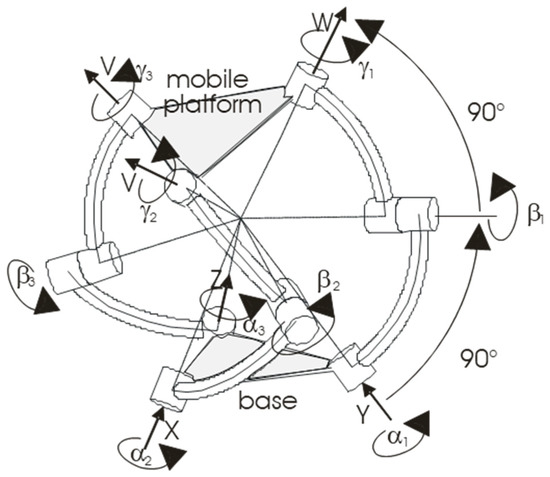
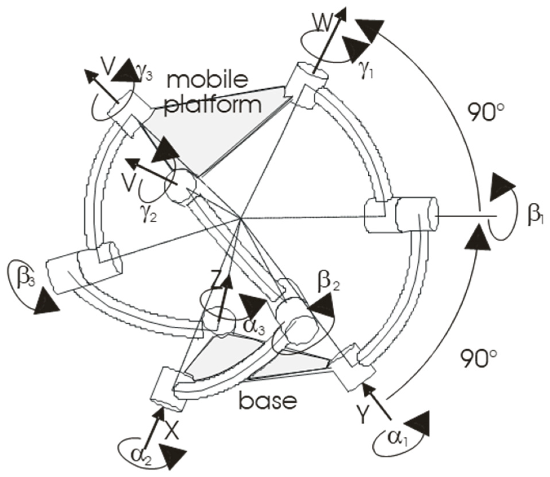
Figure 1.
The kinematic structure of the agile eye.
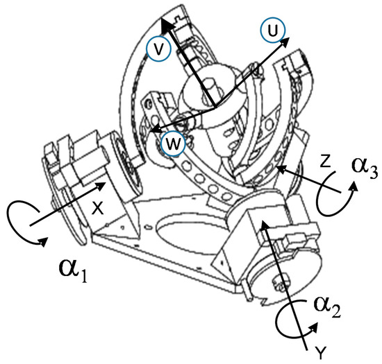
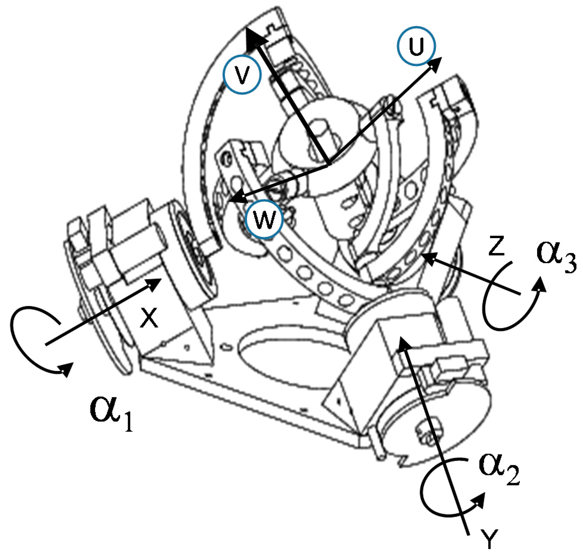
Figure 2.
The agile eye (Adapted from [7]).
The properties of the projective angles can be used to describe the 3D rotation motion of any rigid body and, in this sense, are general. It is a particular angular convention with pros and cons, as with any other convention (Euler angles, quaternions…).
The application to PKM is particularly convenient to the class of spherical manipulators based on rotational joints forming cardan sequences, because in this case, the angles of the angular convention coincide with the joint angles of the PKM.
One example of the second class is the 3-DOF 3SPS/S that is presented in [8,9,10,11], which has three legs with spherical-prismatic-spherical-joints and one additional spherical joint connecting the mobile platform to the fixed base. Another example is described in [12,13], and it is shown in Figure 3. This PKM (better described in the following paragraphs of this paper) can be considered a non-overconstrained version of the agile-eye. The legs are serial kinematic chains for which standard methodologies for their analysis are available [14,15].
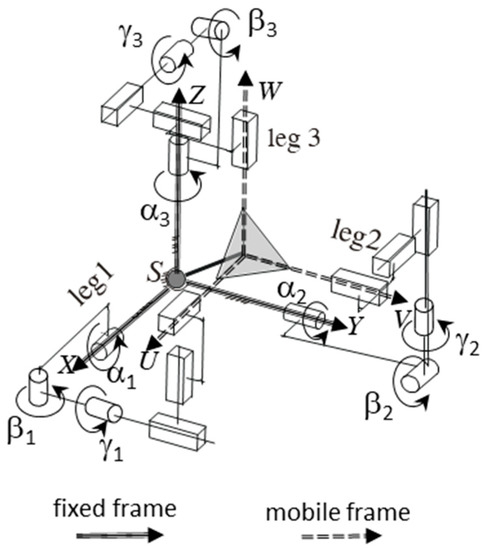
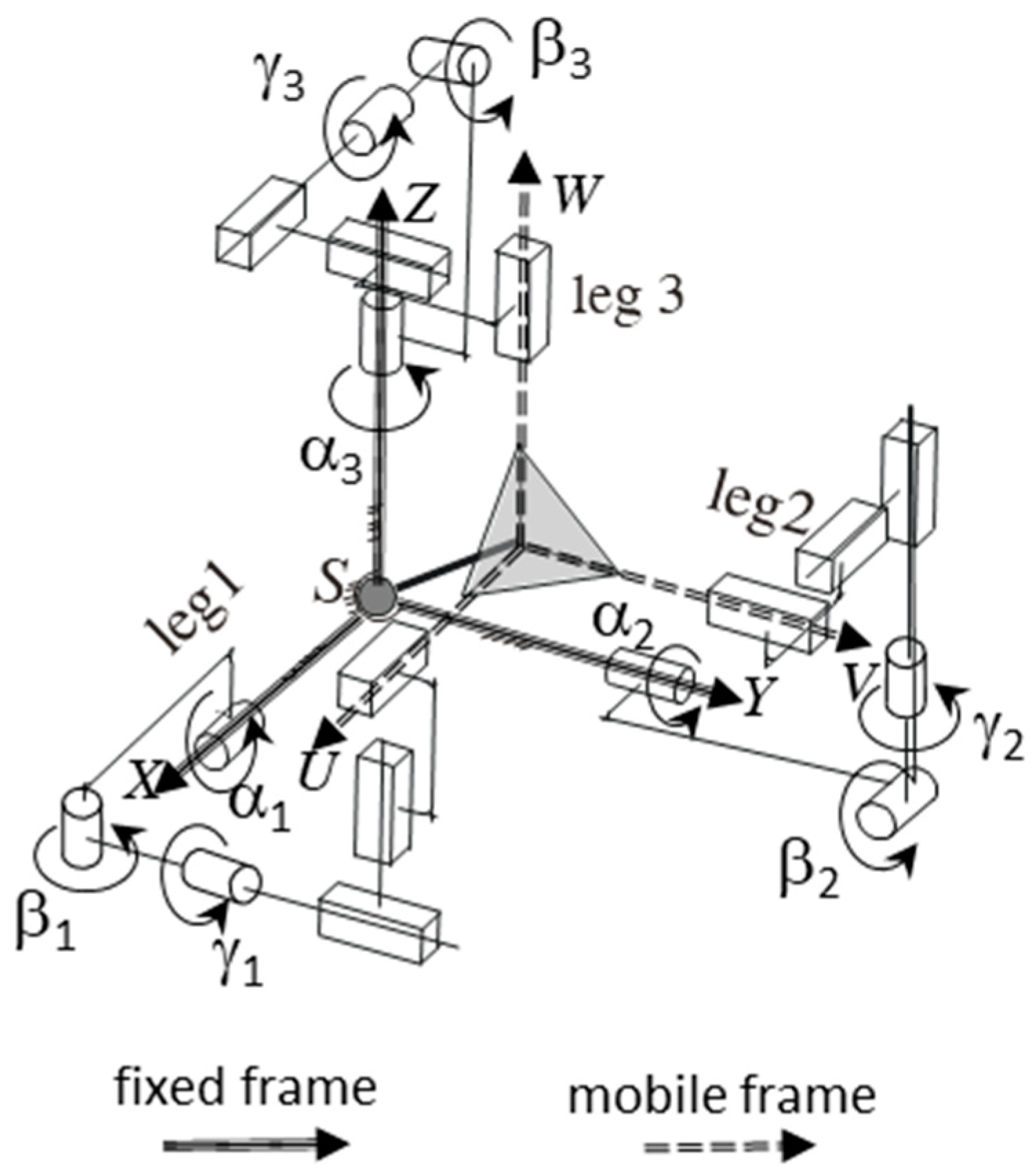
Figure 3.
A non-overconstrained version of the agile-eye.
Several approaches have been developed for the synthesis of the different spherical PKMs. For example, Kong and Gosselin [16,17] proposed the adoption of the screw theory. Fang and Tsai [18] developed a family of spherical PKMs with legs of identical structure, while Karouia and Hervé [19] developed spherical PKMs with legs with different structures. A list with the classification of different spherical manipulators has been suggested by Hess-Coelho [20], which includes a methodology to evaluate their performances. Many other parallel orientation mechanisms have been described in numerous papers (e.g., [3,21,22,23,24,25,26,27,28,29,30,31]). Generally, the first joint of each leg is actuated, however some manipulators adopt transmissions based on parallelograms [31,32].
Analogous concepts were used to design non-redundant PKM with decoupled rotational and translational motion [33] and 2D orientating mechanisms [34,35].
The concept of projective angles has been introduced by [36] and represents a useful approach for the kinematic analysis of PKMs. In [12], this concept has been applied to the angular position analysis of a non-overconstrained variation of the agile eye.
The present paper extends the abovementioned approach to the full kinematic analysis of some spherical PKMs, resulting in a set of easily solvable equations, at position, velocity and acceleration level. Specifically, the proposed approach will be used to solve the direct and inverse kinematics of spherical manipulators, belonging to the two mentioned classes (class A, B).
2. Materials and Methods
2.1. The Agile Eye
The 3RRR agile eye (Figure 1 and Figure 2) is a particular version of a spherical PKM in which the axes of the rotational joints of each link form an angle of 90° and they all converge in one point, which is the centre of rotation.
The mobility of the agile-eye can be studied by the well know Grubler-Kutzbach formula. Having seven bodies and thus, a total of 42 DoF (degrees of freedom) and nine revolute joints for a total of 45 constrains, this means that there are six redundant constrains since the PKM clearly has 3 DoF.
The motion is possible because all of the joint axes converge in one point. The redundant constraints can be removed in several ways by changing the nature of the joints. Recently, a new non-overconstrained version of the agile-eye (Figure 3) was presented in [12].
The mobile platform is connected to the fixed base by three legs having a series of three revolute and three prismatic joints. The first revolute joint of each leg is actuated; in addition, a spherical joint is also present and connects the fixed base and the mobile platform. The PKM is of type 3RRRPPP/S. The joint actuator coordinates of this PKM are the rotations of the actuators that are connected to the first joint of each leg:
where the subscript i = 1, 2, 3 indicates the leg. The rotations of the non-actuated joints are represented by the angles βi and γi. The choice of the name for the angles αi and βi, which is identical to those that we will use for the definitions of the projective angles (see the next section), is justified by the analogies that will be discussed further in this paper.
This PKM can be considered a variant of the agile-eye because the sequences of the revolute joints are the same. The prismatic joints remove the over constraints by leaving three additional translation degrees of freedom which are removed by the spherical joint.
The direct and the inverse kinematics studies the relation between the attitude of the mobile platform and the rotation of the joint actuators, and since the sequence of the joints is the same in the two platforms, their equation may be written in a unified way. Recently, a solution of the position analysis of the PKM of Figure 3 which was based on the concept of the projective angles was presented [12]. Moreover, the possibility to also use projective angles for velocity and acceleration analysis has been proposed in [13]. By joining these results, it is possible to propose a methodology for a full kinematic analysis of the presented class of spherical PKM.
2.2. The Projective Angles
The angular position (attitude) of one body may be represented by the rotation matrix expressing the angular position of a frame that is attached on the body with respect to a fixed frame.
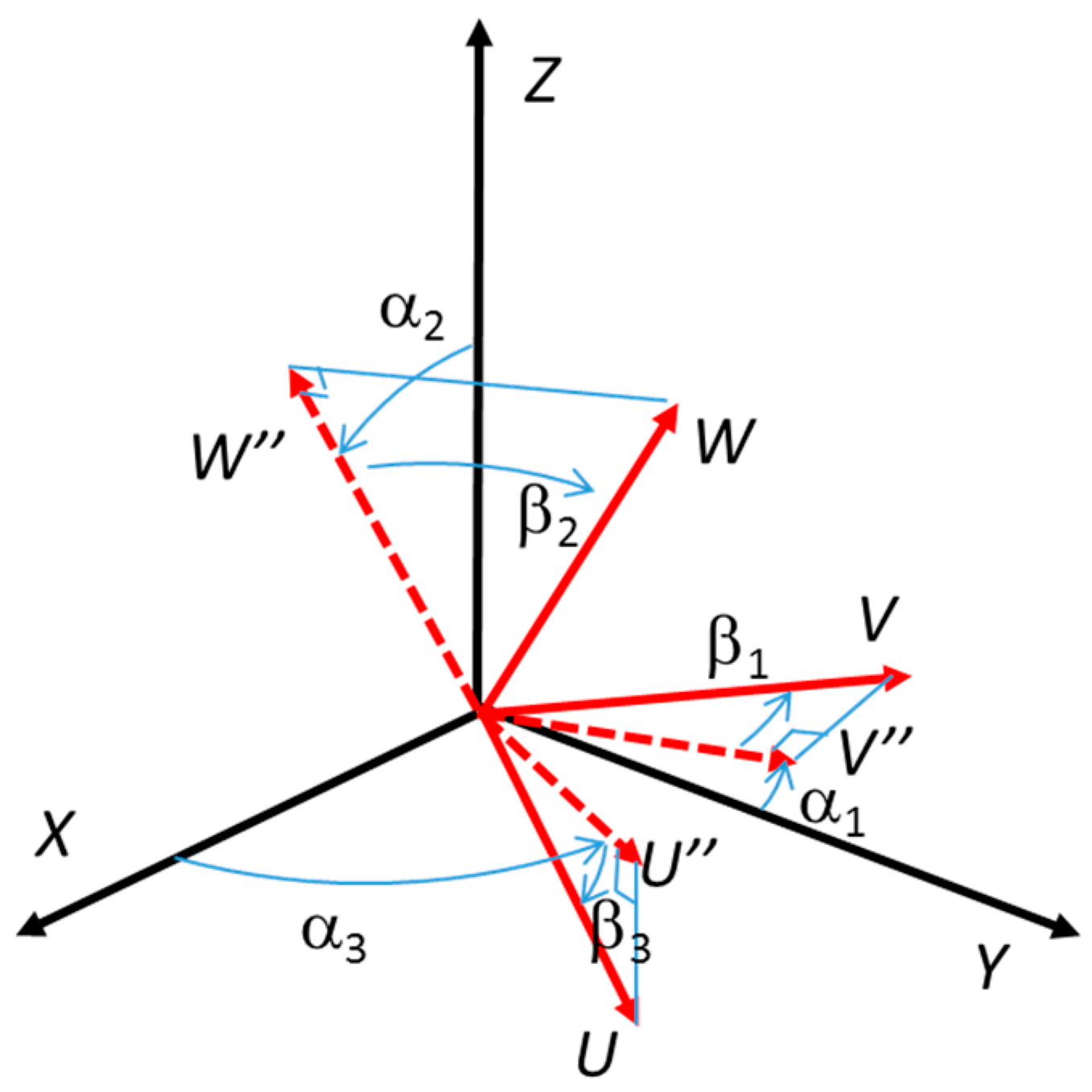
We indicate by X, Y and Z the fixed axes, and by U, V and W the mobile axes (Figure 4, Figure 5 and Figure 6). The rotation matrix is then:

Figure 4.
Definition of the projective angles αi and of the auxiliary angles βi.
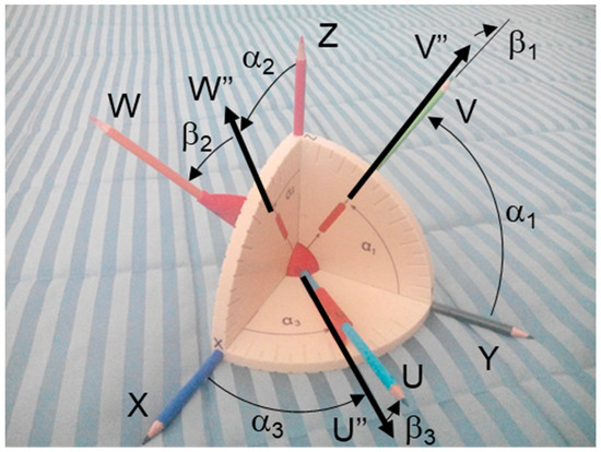
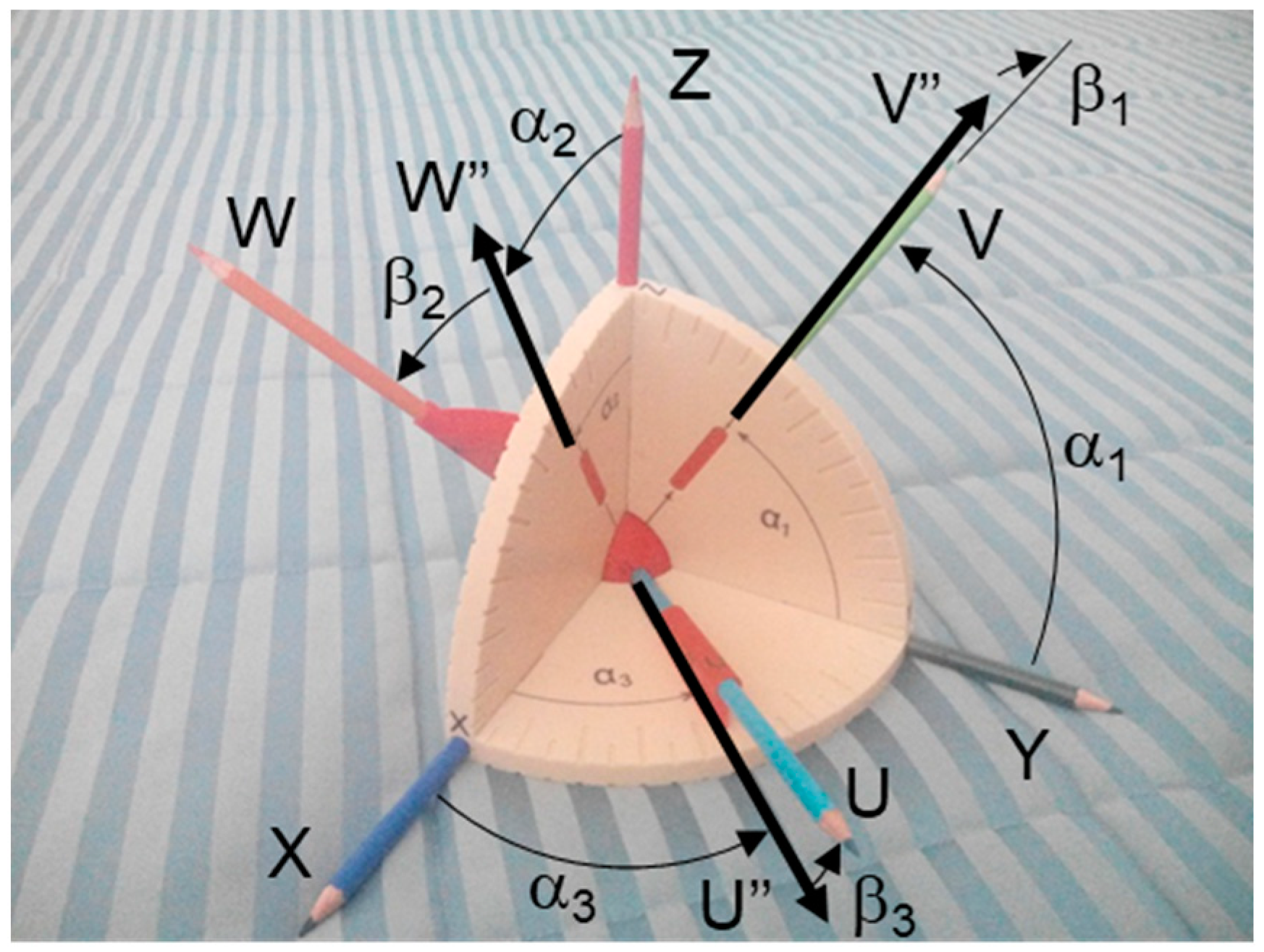
Figure 5.
A 3D model to show the projective angles αi and of the auxiliary angles βi.
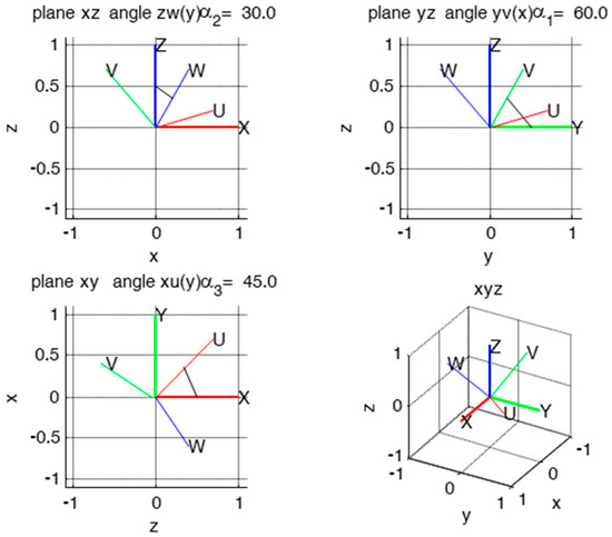
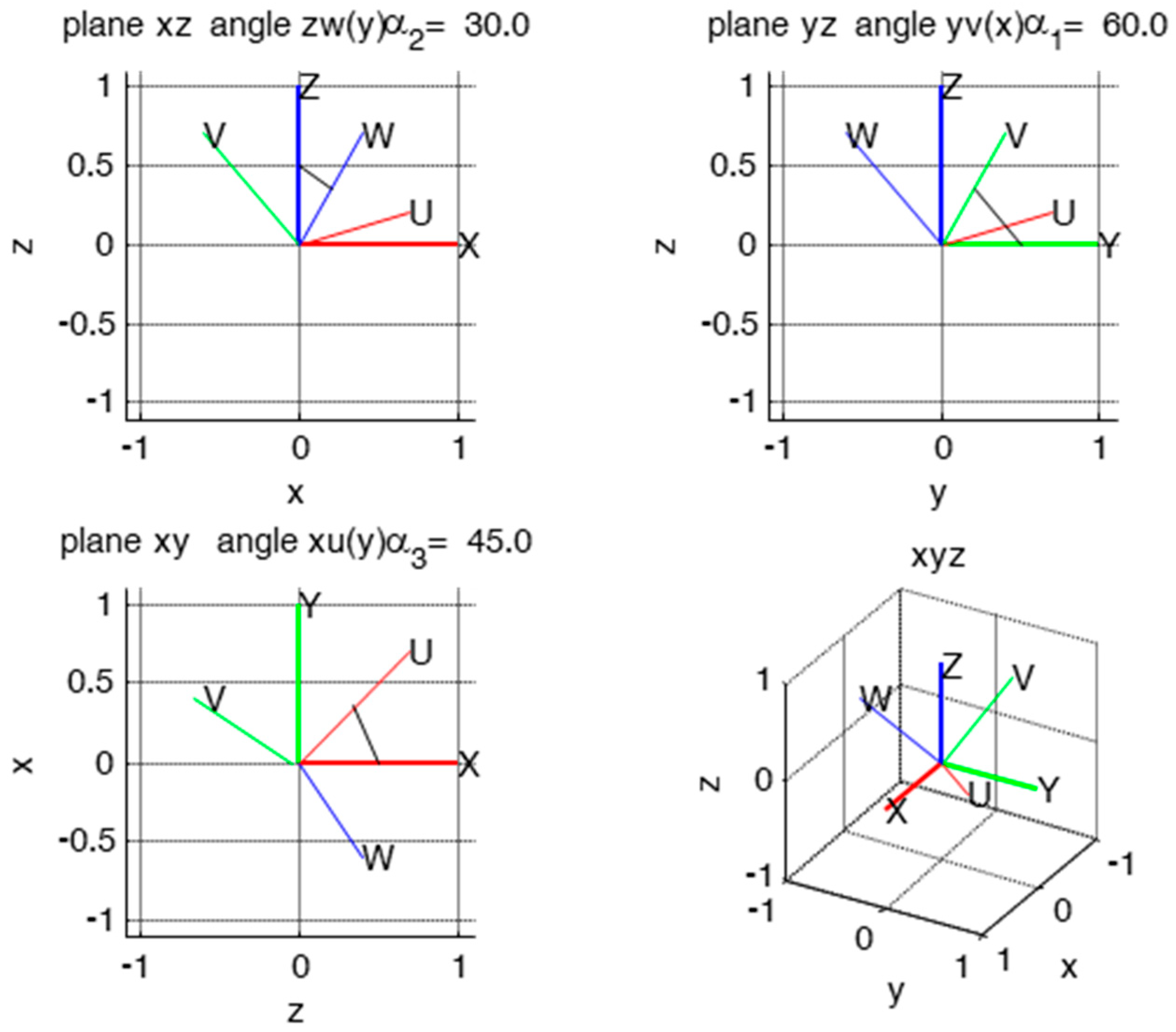
Figure 6.
Visualization of the projective angles on the xy, yz and xz plane; in this example, the projective angles assume the value: 60°, 30°, 45°.
- project the unit vector v of V on plane YZ obtaining vector v”, α1 is the angle between v” and Y;
- project the unit vector w of W on plane XZ obtaining vector w”, α2 is the angle between w” and Z;
- project the unit vector u of U on plane XY obtaining vector u”, α3 is the angle between u” and X.
The definition of the following auxiliary angles β1, β2 and β3 is also necessary for the discussion (Figure 4).
- β1 is the angle between V and the plane YZ
- β2 is the angle between W and the plane XZ
- β3 is the angle between U and the plane XY
and so, the angular position of the mobile frame is:
It is important to note that, by construction, cos(βi) > 0.
The projective angles of the mobile frame may by extracted from the rotation matrix R as:
where atan2(a,b) is the four quadrant extension of the arctangent function atan(a/b). The possibility of using atan2 rather than other inverse trigonometric function (e.g., atan) eliminates the ambiguity of the identification of the correct quadrant and the risk of division by 0.
Therefore, knowing the angular position of the mobile frame (i.e., the rotation matrix R), the projective angles may be easily evaluated. The inverse operation (i.e., determining R when the projective angles are known) will be discussed further in this paper (Section 2.6).
2.3. Inverse Kinematics of the Spherical PKM
To study the mentioned spherical PKM, a fixed frame and a mobile frame were established, as shown in Figure 1, Figure 2 and Figure 3. To simplify the analysis, the coordinate axes are chosen coincidently to the rotation axis of some revolute joints. The XYZ axis of the fixed base frame are parallel with the axes of the actuated joints, while the UVW axes of the mobile frame are parallel with the axis of the joints γi of the mobile frame. The inverse kinematics of the considered spherical PKM can be solved by realizing that the joints of each leg constitute a Cardanic sequence. With reference to Figure 3 and Figure 4, we get:
- leg 1:
- rotations α1β1γ1 around the following axis sequence XZY,
- leg 2:
- rotations α2β2γ2 around YXZ,
- leg 3:
- rotations α3β3γ3 around ZYX.
The rotation matrix R expressing the attitude of the mobile platform can easily be evaluated by considering each different leg. For leg 1, we got:
and similar equations may be written for legs 2 and 3, which lead to the matrices R2 and R3. By indicating the rotation matrix as:
the joint rotations can easily be determined, obtaining two solutions for each leg.
For leg 1 we got:
and similar equations may be written for legs 2 and 3. The relations between the two solutions for the i-th leg is:
and the inverse kinematics is therefore solved by selecting the equations that were associated with the first joint of each leg:
A total of 8 possible solutions were found. Kinematic singularities are present for the configurations for which the atan2 function is not defined, i.e., atan2(0,0) which happens when the second joint angle of one leg is ±90 degrees and so cos(βi) = 0.
2.4. Direct Kinematics
To solve the direct kinematics (find the matrix R when the joint coordinates αi are known), we can write the rotation matrix of the mobile platform by choosing one column for each of the matrix of each leg (Equation (5) for leg 1 and similar equations for the other legs). More precisely, we can bring the second column from R1, the third column from R2 and the first one from R3.
assuming cos(βi) ≠ 0 and dividing each column by the corresponding cos(βi), we got:
with a’ = tgβ1, b’ = tgβ2 and c’ = tgβ3.
Since we are considering the direct kinematics, the angles αi are given, while a’, b’ and c’ can be computed by the conditions of orthogonality of the three columns:
that can be expressed as:
that in matrix form is:
which is a linear system with respect to a’, b’ and c’, of which the solution is:
where , which is the determinant of the linear system that must not be zero for the invertibility of the matrix. Moreover, the determinant must be positive () because the mobile frame is right (for we get a left frame, while results in a singular configuration).
From Equation (15), the value of the angles βi is immediately found:
with ki = 0, 1 and so the direct kinematics has 8 different solutions and matrix R (Equation (10)) is determined.
By only considering the right frames, the singular configurations happened for the following angular position of the mobile platform:
which happens for cos(βi) = 0 and sin(βi) = ±1. For these configurations, the actuated joint angles αi may assume any value.
2.5. Projective Angles and Spherical PKM
An analysis of the definition of the projective angles and of the kinematics of the considered spherical PKM highlights several analogies.
It is worth noting that Equations (4) and (9) are very similar and that they coincide for ki = 0. It is therefore possible to conclude that if for the PKM we choose the solution with cos(βi) > 0, the joint coordinates of the PKM coincide with the projective angles of the mobile platform.
Similarly, the procedure that was adopted to solve the direct kinematics of the PKM can be adopted to compute the angular position of one frame which corresponds to an assigned value of the projective angles αi. In this case, however, we must always assume cos(βi) > 0, and so the solution is unique.
Finally, if we describe the angular position of the mobile platform using the projective angles A, their relation to the joint coordinates Q is:
and so
According to the above equations, and adopting the projective angle convention, the PKM can be considered ‘decoupled’, in the sense that each actuator influences just one of the end-effector coordinates [37]. Therefore, for ki = 0, the joint coordinates of the PKM coincide with the projective angles of the mobile frame and also the angle βi that was used in the description of the projective angles and in the spherical PKM (2nd joint of each leg) have the same values. If the 2nd solution is chosen for the PKM, its angles αi and βi differ from those of the projective angles by 180° (see Equation (21) for analogy). Of course, due to the non-integrability of the angular velocity vector Ω it is:
because it is impossible to define a set of angular coordinates representing a 3D orientation of one body which has a time derivative that coincides with its angular velocity Ω [37,38,39].
A broader analysis of velocity and acceleration is found in the next sections. The analysis will be performed with reference to the abovementioned PKMs; by remembering Equation (21), the results are immediately extended to the projective angles.
We may conclude that the projective angles are a sort of “intrinsic” notation to study the considered spherical PKMs.
2.6. From Projective Angle to Rotation Matrix
Considering the analogies between the kinematic of the spherical PKM and the projective angles, the rotation matrix R that is associated with a set of projective angles A is found by Equations (10) and (16) assuming k1 = k2 = k3 = 0 since, by definition of the projective angles, the cosine of the angles βi are positive.
2.7. Velocity Analysis
Since the legs of the PKM form a Cardanic sequence, the velocity analysis is easily developed. The solution proposed in the following can be applied both to the spherical PKM under study and to the projective angles.
By considering the different legs, we have a first rotation α around one Cartesian axis, a second β rotation around an axis rotated by α and, finally, a third rotation γ around one axis which depends on α and β. For instance, for leg 1, the three rotation axes are defined by the following unit vectors a11 = [1 0 0]t, a12 = [0 − sinα1 cosα1]t and a13 = [−sinβi cosα1 cosβi sinα1 cosβi]t; therefore, for the three legs, and representing the angular velocity of the frame by , we obtain the following results
And so, for leg 1, it is:
and similar equations may be written for legs 2 and 3. The above presented equations may be inverted as:
By considering the first row of the matrix of Equation (26) and the analogous equations for leg 2 and 3, the velocity of the actuated joints is then obtained by the angular velocity of the mobile platform:
while the angular velocity of the end-effector is obtained by the angular velocity of the actuators by inverting the equation:
where .
Equations (27) and (28) are defined for all of the non-singular configurations (for direct or inverse kinematics), which implies:
2.8. Acceleration Analysis
The acceleration analysis may be developed by starting from the velocity relation Equation (27) which synthetically reads:
by a derivation with respect to the time, we found that the joint actuators acceleration was necessary to give an angular acceleration to the end-effector:
and inversely, the angular acceleration of the mobile platform is:
With
where Ca and Cb are:
The time derivatives of the angles βi to be inserted in Cb are easily obtained from Equation (26) and those for legs 2 and 3 as:
The proposed solution can be applied both to the spherical PKM under study and to the projective angles.
3. Results
This paper has presented a methodology for the full kinematics analysis of a class of spherical PKMs. This methodology takes advantage of the properties of the projective angles for which the analysis is extended to velocity and acceleration. All of the solutions are found and the singular cases are discussed.
4. Discussion
The properties of the projective angles can be used to describe the 3D rotation motion of any rigid body and, in this sense, this notation is general. It is a particular angular convention with pros and cons, as with any other convention (Euler angles, quaternions…). The application to PKM is particularly convenient to the class of spherical manipulators based on rotational joints forming cardan sequences because, in this case, the angles of the angular convention coincide with the joint angles of the PKM. In this context, the paper highlights the numerous analogies between the direct and inverse kinematics of the PKM and the relations between the rotation matrix describing the orientation of the end-effector and the projective angles of the frame that were associated with it. We may conclude that the projective angles are a sort of “intrinsic” notation to study the considered spherical PKMs.
The paper solves this relation for angular position, velocity and acceleration.
The proposed methodology is an alternative solution to those that were proposed by classical papers.
The inverse kinematics analysis of the agile eye, as reported in [1], results, for any actuated joint, in a quadratic equation of the tangent of the angle of the corresponding joint rotation. With the proposed methodology, if we adopt the projection angles as angular convention, we do not need to perform calculations because the actuated joint rotation coincides with the projective angles of the mobile frame, therefore there is no need to perform calculations.
The direct analysis of the agile eye is reported in [2] and results in a polynomial of degree 8 which leads to 8 real solutions. When adopting the methodology that was proposed in this paper, it is necessary to solve a 3 × 3 linear system instead and optionally to add ±180° to the angles to generate the different solutions.
The problem that was addressed in the paper has multiple solutions, both for direct and inverse kinematics. The chosen solution can be selected according to common robotic practice: each solution corresponds to a different assembly configuration. Different configurations can be reached by crossing a singular configuration. Since this operation may create control problems in the execution of trajectories generally, at each time, the “most close” configuration with respect to the current configuration is chosen. So, for direct kinematics, if R is the actual configuration at time T and R1’, R2’,… are the different solutions for t = T + dT, the i-th solution chosen is the one that minimizes . A similar approach can be applied to the inverse kinematics minimizing the rotation of the motors to reach the next pose. This also ensures the absence of discontinuity in the joint motion.
If the angular position of the end-effector is represented by projective angles, the Jacobian matrix is the identity matrix and therefore, in the domain of the projective angles, the PKM can be defined as decoupled.
Author Contributions
Conceptualization, G.L. and I.F.; Writing—Original Draft Preparation, G.L. and I.F., Writing-Review & Editing G.L., Project Administration, I.F.
Funding
Project Evolut and UniBS ex 60%.
Acknowledgments
The 3D model of Figure 5 was designed and fabricated by Giulio Spagnuolo (ITIA-CNR). His cooperation is greatly appreciated.
Conflicts of Interest
The authors declare no conflict of interest. The funders had no role in the design of the study; in the collection, analyses, or interpretation of data; in the writing of the manuscript, and in the decision to publish the results.
References
- Gosselin, C.; Angeles, J. The Optimum Kinematic Design of a Spherical Three-Degrees-of-Freedom Parallel Manipulator. ASME J. Mech. Trans. Autom. Des. 1989, 111, 202–207. [Google Scholar] [CrossRef]
- Gosselin, C.M.; Sefrioui, J.; Richard, M.J. On the direct kinematics of spherical three-degree-of-freedom parallel manipulators of general architecture. ASME J. Mech. Des. 1994, 116, 594–598. [Google Scholar] [CrossRef]
- Gosselin, C.M.; Lavoie, E. On the kinematic design of spherical three-degree-of-freedom parallel manipulators. Int. J. Robot. Res. 1993, 12, 394–402. [Google Scholar] [CrossRef]
- Kong, X.; Gosselin, C.M. A formula that produces a unique solution to the forward displacement analysis of a quadratic spherical parallel manipulator: The Agile Eye. ASME J. Mech. Robot. 2010, 2, 044501. [Google Scholar] [CrossRef]
- Malosio, M.; Pio Negri, S.; Pedrocchi, N.; Vicentini, F.; Caimmi, M.; Molinari Tosatti, L. A Spherical Parallel Three Degrees-of-Freedom Robot for Ankle-Foot Neuro-Rehabilitation. In Proceedings of the 34th Annual International Conference of the IEEE EMBS, San Diego, CA, USA, 28 August–1 September 2012. [Google Scholar]
- Malosio, M.; Caimmi, M.; Ometto, M.; Molinari Tosatti, L. Ergonomics and kinematic compatibility of PKankle, a fully-parallel spherical robot for ankle-foot rehabilitation. In Proceedings of the 5th IEEE RAS & EMBS International Conference on Biomedical Robotics and Biomechatronics (BioRob), São Paulo, Brazil, 12–15 August 2014. [Google Scholar]
- Gosselin, C.M.; St. Pierre, E.; Gagné, M. On the development of the Agile Eye. IEEE Robot. Autom. Mag. 1996, 3, 29–37. [Google Scholar] [CrossRef]
- Innocenti, C.; Parenti-Castelli, V. Echelon Form Solution of Direct Kinematics for the General Fully-Parallel Spherical Wrist. Mech. Mach. Theory 1993, 28, 553–561. [Google Scholar] [CrossRef]
- Wohlhart, K. Displacement Analysis of the General Spherical Stewart Platform. Mech. Mach. Theory 1994, 29, 581–589. [Google Scholar] [CrossRef]
- Huang, Z.; Yao, Y.L. A New Closed-Form Kinematics of the Generalized 3-DOF Spherical Parallel Manipulator. Robotica 1999, 17, 475–485. [Google Scholar] [CrossRef]
- Alici, G.; Shirinzadeh, B. Topology Optimisation and Singularity Analysis of a 3-SPS Parallel Manipulator with a Passive Constraining Spherical Joint. Mech. Mach. Theory 2004, 39, 215–235. [Google Scholar] [CrossRef]
- Kuo, C.-H.; Dai, J.S.; Legnani, G. A non-overconstrained variant of the Agile Eye with a special decoupled kinematics. Robotica 2014, 32, 889–905. [Google Scholar] [CrossRef]
- Legnani, G.; Fassi, I. Representation of 3D Motion by Projective Angles. In Proceedings of the ASME IDETC2015, Boston, MA, USA, 2–5 August 2015. [Google Scholar]
- Legnani, G.; Casolo, F.; Righettini, P.; Zappa, B. A homogeneous matrix approach to 3D kinematics and dynamics—I. Theory. Mech. Mach. Theory 1996, 31, 573–587. [Google Scholar] [CrossRef]
- Legnani, G.; Casolo, F.; Righettini, P.; Zappa, B. A homogeneous matrix approach to 3D kinematics and dynamics—II. Applications to chain of rigid bodies and serial manipulators. Mech. Mach. Theory 1996, 31, 589–605. [Google Scholar] [CrossRef]
- Kong, X.; Gosselin, C.M. Type Synthesis of Three-Degree-of-Freedom Spherical Parallel Manipulators. Int. J. Robot. Res. 2004, 23, 237–245. [Google Scholar] [CrossRef]
- Kong, X.; Gosselin, C.M. Type Synthesis of 3-DOF Spherical Parallel Manipulators Based on Screw Theory. ASME J. Mech. Des. 2004, 126, 101–126. [Google Scholar] [CrossRef]
- Fang, Y.; Tsai, L.-W. Structure Synthesis of a Class of 3-DOF Rotational Parallel Manipulators. IEEE Trans. Robot. Autom. 2004, 20, 117–121. [Google Scholar] [CrossRef]
- Karouia, M.; Hervé, J.M. Asymmetrical 3-Dof Spherical Parallel Mechanisms. Eur. J. Mech. A Solids 2005, 24, 47–57. [Google Scholar] [CrossRef]
- Hess-Coelho, T.A. Topological Synthesis of a Parallel Wrist Mechanism. ASME J. Mech. Des. 2006, 128, 230–235. [Google Scholar] [CrossRef]
- Karouia, M.; Hervé, J.M. A Three-DOF Tripod for Generating Spherical Rotation. In Advances in Robot Kinematics; Lenarčić, J., Stanišić, M.M., Eds.; Springer: Basel, Switzerland, 2000; pp. 395–402. [Google Scholar]
- Di Gregorio, R. Kinematics of a New Spherical Parallel Manipulator with Three Equal Legs: The 3-URC Wrist. J. Robot. Syst. 2001, 18, 213–219. [Google Scholar] [CrossRef]
- Di Gregorio, R. A New Parallel Wrist Using Only Revolute Pairs: The 3-RUU Wrist. Robotica 2001, 19, 305–309. [Google Scholar] [CrossRef]
- Di Gregorio, R. A New Family of Spherical Parallel Manipulators. Robotica 2002, 20, 353–358. [Google Scholar] [CrossRef]
- Di Gregorio, R. Kinematics of the 3-UPU Wrist. Mech. Mach. Theory 2003, 38, 253–263. [Google Scholar] [CrossRef]
- Di Gregorio, R. The 3-RRS Wrist: A New, Simple and Non-Overconstrained Spherical Parallel Manipulator. ASME J. Mech. Des. 2004, 126, 850–855. [Google Scholar] [CrossRef]
- Di Gregorio, R. Kinematics of the 3-RSR wrist. IEEE Trans. Robot. 2004, 20, 750–753. [Google Scholar] [CrossRef]
- Karouia, M.; Hervé, J.M. Non-Overconstrained 3-Dof Spherical Parallel Manipulators of Type: 3-RCC, 3-CCR, 3-CRC. Robotica 2006, 24, 85–94. [Google Scholar] [CrossRef]
- Gogu, G. Fully-Isotropic Three-Degree-of-Freedom Parallel Wrists. In Proceedings of the IEEE International Conference on Robotics and Automation, Rome, Italy, 10–14 April 2007; pp. 895–900. [Google Scholar]
- Enferadi, J.; Tootoonchi, A.A. A Novel Spherical Parallel Manipulator: Forward Position Problem, Singularity Analysis, and Isotropy Design. Robotica 2009, 27, 663–676. [Google Scholar] [CrossRef]
- Baumann, R.; Maeder, W.; Glauser, D.; Clavel, R. The PantoScope: A Spherical Remote-Center-of-Motion Parallel Manipulator for Force Reflection. In Proceedings of the IEEE International Conference on Robotics and Automation, Albuquerque, NM, USA, 20–25 April 1997; pp. 718–723. [Google Scholar]
- Vischer, P.; Clavel, R. Argos: A Novel 3-DoF Parallel Wrist Mechanism. Int. J. Robot. Res. 2000, 19, 5–11. [Google Scholar] [CrossRef]
- Kuo, C.-H.; Dai, J.S. Kinematics of a Fully-Decoupled Remote Center-of-Motion Parallel Manipulator for Minimally Invasive Surgery. ASME J. Med. Devices 2012, 6, 021008. [Google Scholar] [CrossRef]
- Carricato, M.; Parenti-Castelli, V. A Novel Fully Decoupled Two-Degrees-of-Freedom Parallel Wrist. Int. J. Robot. Res. 2004, 23, 661–667. [Google Scholar] [CrossRef]
- Gallardo, J.; Rodríguez, R.; Caudillo, M.; Rico, J.M. A Family of Spherical Parallel Manipulators with Two Legs. Mech. Mach. Theory 2008, 43, 201–216. [Google Scholar] [CrossRef]
- Kuo, C.-H. Projective-Angle-Based Rotation Matrix and Its Applications. In Proceedings of the Second IFToMM Asian Conference on Mechanism and Machine Science, Tokyo, Japan, 7–10 November 2012. [Google Scholar]
- Legnani, G.; Fassi, I.; Giberti, H.; Cinquemani, S.; Tosi, D. A new isotropic and decoupled 6-DoF parallel manipulator. Mech. Mach. Theory 2012, 58, 64–81. [Google Scholar] [CrossRef]
- Angels, J. Rational Kinematics; Springer: London, UK, 1988. [Google Scholar]
- Nappo, F. On the absence of a general link between the angular velocity and the characterization of a rigid displacement. Rendiconti di Matematica 1970, 3. Series VI. [Google Scholar]
© 2018 by the authors. Licensee MDPI, Basel, Switzerland. This article is an open access article distributed under the terms and conditions of the Creative Commons Attribution (CC BY) license (http://creativecommons.org/licenses/by/4.0/).