Optimizing Path Planning for Automated Guided Vehicles in Constrained Warehouse Environments: Addressing the Challenges of Non-Rotary Platforms and Irregular Layouts

Abstract

Efficient path planning for Automated Guided Vehicles (AGVs) in warehouse automation is crucial yet challenging, particularly in environments with irregular structures and constrained spaces. This study addresses these challenges by focusing on AGVs without rotary platforms, which require the rotation of the entire robot-rack assembly for directional changes, demanding additional space and complex path planning. We have developed dedicated algorithms that integrate robotics and optimization principles to tackle these issues. Our methods take into account the spatial requirements for rack rotation, navigating through limited inter-rack clearance, and adapting to irregular warehouse layouts. Extensive simulations and real-world applications validate the proposed solutions, demonstrating significant improvements in traversal efficiency and collision risk mitigation. The results indicate that our algorithms effectively enhance the operational efficiency and reliability of AGV systems in complex warehouse environments. This research adapts AGV path planning by providing robust strategies to optimize navigation in challenging settings, ultimately improving warehouse productivity.

1. Introduction

1.1. Problem Background

The construction of multi-agent robotic systems is an actively developing field of science involving researchers from various specialties. Such systems are based on various architectural and algorithmic paradigms. Such systems can be characterized by varying degrees of centralization [1] and use different models to plan the activities of individual robots. One popular solution is the use of game theory [2,3] often connected with adaptive control techniques [4,5]. In less complex situations, following the famous “Planning is Just a Way of Avoiding Figuring Out What to Do Next” [6], a reactive approach is used [7]. The control of multi-robot systems can be subject to attacks and disruptions [8,9,10]. Such systems can also perform many tasks, from delivering pizzas (https://www.theguardian.com/technology/2016/mar/18/dominos-unveil-worlds-first-pizza-delivery-robot, accessed on 25 March 2025) and interacting in production systems [11] to supporting the operation of goods storage facilities—warehouses. In this article, we want to focus on the latter in the context of path planning in a centralized multi-robot system.

Warehouse automation is increasingly critical in today’s world. Millions of people are employed in warehouses globally, but with the rapid growth in global logistics demands, the need for workers could substantially increase in the coming years. Logistics companies are already facing a labor shortage. The global logistics market is valued at hundreds of billions of dollars, with warehouse automation and robot-assisted automation markets being significant subsets of this value. According to research, the warehouse automation market is expected to grow exponentially in the coming decades. Currently, only a tiny percentage of warehouses worldwide are automated, with the majority relying on human labor. Workers in warehouses often walk long distances daily, and the turnover rate is high, with many employees quitting within the first year. On average, it takes a human significantly more time to process one item in a fulfillment warehouse than robots, which can process items much faster. Robots significantly enhance human efficiency; under ideal conditions, they can substantially reduce the number of required workers as they handle the movement of goods and packages. The main barriers to robotics development are the complexity of implementation, maintenance costs, and the effectiveness of solutions. Each year, improvements are made in all these areas. It is crucial to note that the cost of robots, a key parameter for calculating project payback, is significantly lower for simpler robotic systems compared to more complex ones. It is also important to note that automation impacts both large warehouses designed explicitly for such needs and existing ones that were not initially intended for robotic operations. This research aims to address this gap in the vast field of robotics, providing solutions that can be applied to a broader range of warehouse environments.

1.2. Problem Definition

In warehouse environments, especially those not designed initially for robotic operations and later retrofitted for such use, space constraints and the absence of rotary platforms in robots create significant challenges for pathfinding and collision avoidance. Environmental factors, like narrow aisles or irregular layouts, and obstacles, such as columns or mezzanine structures, further complicate navigation. The inability of non-rotary robots to turn in place demands even more precise path planning, particularly in tightly packed storage areas with limited maneuvering space.

The problem of finding conflict-free paths for a group of agents, known as Multi-Agent Path Finding (MAPF), has received significant attention over the last decade [12,13,14]. Early MAPF algorithms were capable of building paths for a few agents [12] or producing low-quality solutions [15], but modern solutions can now control thousands of robots [16]. The MAPF problem is NP-hard [17], so all existing solutions rely on specific assumptions that trade solution quality for speed. In contrast, others focus on solving the problem for a smaller number of agents by incorporating some real-world characteristics of the agents. Unlike modern facilities optimized for robot usage, older warehouses present unique challenges due to their irregular and constrained spaces. While existing research has explored the challenges of large agents and irregular environments, our approach builds on these studies by modifying and integrating several specific concepts to develop a relatively simple yet highly efficient algorithm for the described problem.

1.3. Related Work

1.3.1. Classical Multi-Agent Path Finding Problem

Multi-Agent Path Finding (MAPF) involves constructing a collision-free path for a group of agents. Following the definition given by Stern et al. [17], let us consider a tuple $<G,s,t>$ for k agents, where $G=(V,E)$ is an undirected graph, $s:\left\{1,\dots ,k\right\}\to V$ maps an agent to a source vertex, and $t:\left\{1,\dots ,k\right\}\to V$ maps an agent to a target vertex. Time is assumed to be discrete and, at each time step, every agent occupies one of the graph vertices. At each time step, the agent can perform a single action. The action is a function $a:V\to V$ such that if $a\left(v\right)=v^{\prime }$ and an agent is at vertex v performing action a, then the agent will be at vertex $v^{\prime }$ at the next time step. Usually, there are two types of actions: wait and move. Wait means that the robot stays in the same vertex in the next time step, whereas move means changing the vertex to one of the adjacent vertices in the initial graph V.

For the sequence of actions $\pi =\left(a_1,a_2,...,a_n\right)$ and agent i, the position of the agent at time T is defined as ${\pi }_i\left(T\right)=a_T\left(a_{T-1}\left(\cdots a_1\left(s\left(i\right)\right)\right)\right)$. A sequence ${\pi }_i$ is a single-agent plan for agent i if ${\pi }_i\left(T\right)=t\left(i\right)$ for some time step T. A solution is a set of k single-agent plans, one for each agent.

1.3.2. Multi-Agent Path Finding for Large Agents (LA-MAPF)

With Multi-Agent Path Finding for Large Agents, Li et al. [18] extend the classical MAPF problem by addressing the complexities involved when agents occupy more than one vertex, unlike traditional MAPF, which assumes that each agent fits within a single cell. This extension is necessary for scenarios involving large robots, drones, or vehicles that may occupy multiple positions on a grid simultaneously, requiring the more sophisticated handling of movement and collision avoidance.

1.3.3. Search-Based Solvers

As noted in [19], the MAPF problem can be solved by various methods, including reduction to Boolean Satisfiability, Integer Linear Programming, and Answer Set Programming. Another class of MAPF algorithms consists of search-based solvers, which search through the solution in a coupled manner among agents. According to [17,20], search-based solvers can be divided into three main categories:

• $A^{*}$-based algorithms: Algorithms of this class include $A^{*}$ with k-agent search space, Operator Decomposition, Independence Detection, $M^{*}$, and others. The main drawback of this class of algorithms is a lack of scalability due to the large search space.
• CBS-based algorithms: Conflict-Based Search (CBS) algorithms form a class of two-level search strategies. The low-level search is used to find a path for a single agent, and the high-level search is used for conflict resolution for paths obtained during the low-level search. This class includes CBS that is complete and optimal [21], ECBS (Enhanced CBS), a bounded-suboptimal variant of CBS [22], and EECBS (Explicit Estimation CBS), yet another bounded-suboptimal variant of CBS [23].
• Prioritized algorithms: The main idea of prioritizing planning algorithms is to select random agent ordering and find a minimum cost path for each agent according to the chosen priority [12]. If, at some moment, the path for agent $a_i$ cannot be constructed in such a way that it has no collisions with the path of agents with higher priority, then new ordering is selected, and the search is restarted. The adaptation of CBS to prioritized planning, named Conflict-Based Search with Priorities (CBSwP), and Priority-Based Search (PBS) are proposed in [24].

1.3.4. Multi-Label $A^{*}$

When dealing with agents’ behavior at the target locations, classical MAPF usually considers two cases: staying at the target location or disappearing. In the case of lifelong MAPF, both cases add additional constraints on task assignment.

• The ‘stay at the target’ approach prohibits other agents from entering the target location, which limits the number of simultaneously processed orders with the same destination to one.
• Disappearing at the target avoids the first problem, but some agents can block the path for the agent that leaves the target location. In both cases, additional heuristics or modifications should be added to algorithms.

To avoid the problems described above, a multi-label extension of the $A^{*}$ algorithm was proposed in [25]. This algorithm combines the search for a path to the pickup location with the search for paths to the delivery location or an ordered sequence of delivery locations.

1.3.5. Windowed Approach

As MAPF problems are not solvable in the polynomial time, Silver [12] proposed building partial routes for each agent by limiting the cooperative search depth to the fixed depth while the abstract search is executed in full. He empirically showed that his algorithm ${\mathrm{WHCA}}^{*}$ runs faster as the agents conflict with each other during the limited time interval. Later, Li et al. [26] applied this idea to lifelong MAPF and other MAPF solvers. A new framework named Rolling-Horizon Collision Resolution (RHCR) showed the ability to produce high-quality solutions for up to 1000 agents.

1.3.6. MAPF Extensions

• Kinematic constraints: In the classical case, all agents in MAPF occupy a single vertex of the graph, but in real-world scenarios, each vertex of the graph has Euclidean coordinates, and agents may be prohibited from being in some pair of vertices due to their geometrical shapes or shapes of the attached loads. Any-angle SIPP was proposed by Yakovlev et al. [27] to deal with multiple agents of identical circular shape. Further research in this direction includes MC-CBS [18], a generalized version of CBS, and TP-SIPPwRT [28], an adaptation of Token Passing [19] that uses SIPPwRT as low-level search and takes kinematic constraints into account. MAPF-POST [29] adds a post-processing step where robot kinematics are considered.
• Rotations as separate actions: Standard MAPF operates only with graph vertices, and robot direction is not considered. Honig et al. [30] proposed an execution framework where robot rotations are used to model the rotation time and explicitly achieve more accurate plans. This approach also allows the consideration of kinematic constraints and finding collisions when the robot is planned to make a rotation near another robot or obstacle. However, this increases the search space because each robot’s position is now encoded with location and direction. On the other hand, as discovered in [20], rotations as separate actions can improve the throughput of ECBS-T and PP.
• k-Robustness: To deal with unexpected events that delay plan execution, Artzmon et al. [31] proposed the k-robust MAPF plan: a plan that can be executed even if a limited number $\left(k\right)$ of delays occur and adopted some MAPF solvers to use the k-Robustness constraint. This is achieved by redefining vertex conflict in such a way that if the agents share the same cell in within fewer than $k-1$ time steps, then these agents conflict with each other. This approach increases computational time compared to non-robust $(k=0)$ variants and increases the failure rate for prioritized planning algorithms but can produce higher throughput for some instances [20]. In addition, we should point out that k-Robustness implies that there are no edge conflicts.

1.3.7. Lifelong MAPF

Classical MAPF formulation deals with cases when all initial and final configurations are fixed. After reaching the goal vertex, agents can wait indefinitely or disappear at their final locations [17]. In real-world scenarios, such as warehouses or sorting centers, where robots move some loads from one location to another, not all the tasks are known in advance and can appear from time to time. The latter is referred to as lifelong MAPF [19]. Lifelong MAPF extends the classical MAPF problem to scenarios where tasks appear dynamically in real time. Agents must continuously adapt their plans to accommodate newly introduced tasks while maintaining efficiency and avoiding conflicts. This dynamic nature introduces additional complexities, requiring algorithms capable of online planning and replanning to handle changing task demands effectively.

Sometimes, lifelong MAPF with task assignments is considered. This variant of the problem is called multi-agent pickup and delivery (MAPD) [19]. In the MAPD problem, the tasks appear in an online setting and must be assigned to the agents along with the construction of collision-free paths.

There are a variety of different techniques to solve the problem. Next, we provide a short description of some of them:

• Reducing the problem to one-shot MAPF: If all the tasks are known beforehand, optimal or near-optimal solvers can generate a complete solution considering all tasks and agent interactions. Once a new navigation task is assigned, the new problem should be solved again in an offline setting. A further extension of this idea is replicating agents that receive new tasks (Online Independence Detection [32]) or reusing the previous search results.
• Decoupled (single-agent) frameworks: The idea is not new and quite simple. Agents plan their paths one after another, avoiding collision with already planned paths. Examples of such an approach are Cooperative $A^{*}$ [12], Token Passing (TP) and Token Passing with Tasks Swaps (TPTS) [19], and Token Passing using SIPP (TP-SIPPwRT) [28]. For this purpose, paths are stored in a global reservation system consisting of space-time cells. Each agent needs to reserve a cell at some time step to be available to move there and every cell can be reserved at most by one agent.
• Windowed solvers (Bounded-Horizon Planning): Another approach is based on constructing collision-free paths only for a limited number of steps w using any of the MAPF algorithms. Replanning is triggered after $h<w$ steps or when some new tasks are added to the system. Windowed solvers are faster than their complete version but generate longer paths. Examples of algorithms in this category are Windowed Hierarchical Cooperative $A^{*}$ (${\mathrm{WHCA}}^{*}$) [12], and Rolling-Horizon Collision Resolution (RHCR) [26]. Varambally et al. [20] presented an execution framework called Rolling-Horizon Collision-Resolution and Execution (RHCRE), which combines RHCR with an Action-Dependency Graph. In this way, they achieved the same robustness guarantees as single-agent frameworks. They overcame the inaccuracies in the general assumptions of the MAPF problem, such as one-step actions and unpredictable delays. The ADG also allows for replanning during execution, which means that agents do not need to wait during replanning.

1.3.8. Action Dependency Graph

During MAPF solving, researchers try to balance the number of agents and solution quality. More robust schemes require additional assumptions like k-Robustness [31], considering rotations and pick-drop actions [30], using kinematic constraints [18,19,27,28], or continuous time [33].

To avoid additional assumptions on the MAPF instance, Hoenig et al. [29] proposed a Temporal Plan Graph to decode events corresponding to agents entering locations. This algorithm, called MAPF-POST, converts the MAPF plan to plan-execution policies that can be executed on robots. This idea was continued in [30] where the authors defined an Action Dependency Graph (ADG), in which dependencies between states from MAPF-POST are replaced with dependencies on robots actions. Berndt et al. [34] proposed a way to modify ADG in an online setting when considerable delays occur, where agents should wait for an unknown period. Varambally et al. [20] further improved the ADG framework by integrating the Rolling-Horizon Collision-Resolution framework to solve the MAPF problem with a persistent stream of online tasks.

2. Materials and Methods

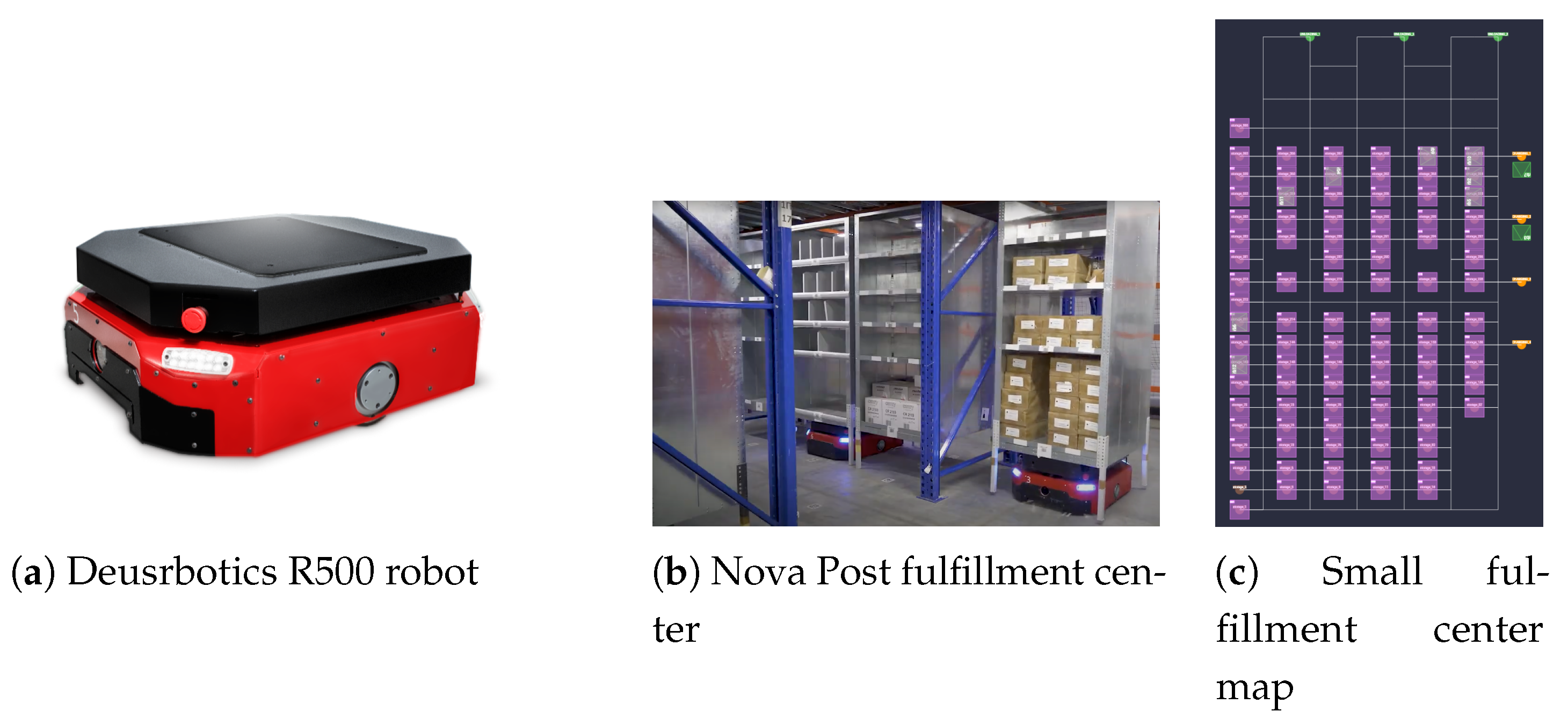
2.1. Environment and Equipment

Automating small warehouse spaces requires paying careful attention to the unique constraints and specifications of the environment and the equipment used, as we cannot drastically alter the warehouse structure to make it more robot friendly. Driven by market demands, we focused on automating small warehouses and postal facilities, where space limitations and budget constraints are critical. One of our earliest robot models was designed without a rotary platform. This choice significantly reduced the product’s cost but added complexity to the algorithmic design and imposed certain operational limitations. This lack of rotational capability meant that every turn required additional space, necessitating strict collision checking during path planning to avoid collisions and ensure efficient navigation in constrained areas.

The specific conditions we worked with are as follows:

• Robot Dimensions: Each robot measures 798 mm in length and 666 mm in width and has a turning diameter of 872 mm. These dimensions are critical for navigating tight spaces and performing precise maneuvers.
• Lack of Rotary Platform: The robots are not equipped with a rotary platform, meaning that rotations require additional space and careful path planning to avoid collisions, especially when the load is attached to the robot.
• Safety sensors at the front: The robot has a 3-D camera, meaning forward movement is preferred, but backward movement is also possible.
• Shelf Dimensions: The shelves used in the warehouse measure 800 mm by 800 mm. Their size must be considered when planning paths and rotations, particularly in constrained areas.
• Storage Point Spacing: The distance between shelf storage points is 900 mm. This spacing affects how robots navigate between shelves and pick up or drop off loads.
• External Obstacles: The warehouse environment includes various external obstacles, such as columns, barriers, and walls. These obstacles prevent an even distribution of storage locations and necessitate flexible path planning to accommodate narrow passages, sometimes as small as 20–30 cm.
• Turn Restrictions: In specific locations, external obstacles prohibit the robot from turning with a shelf, requiring alternative strategies for maneuvering in these areas.
• Flexible Shelf Pickup: The system must accommodate the ability to pick up shelves at designated storage points and any arbitrary location within the warehouse map. This flexibility is crucial for efficient operation and recovery scenarios.

These conditions form the basis for the subsequent formulation of the MAPF problem, where we address the challenges posed by the environment and equipment constraints.

All robots used in the experiments conducted for the purposes of the article were built in the Ukrainian branch of Deus Robotics. The control software was written in C and C++ using the current versions of the CLion IDE from JetBrains, Czech Republic, released in 2023–2025.

2.2. MAPF Problem Setup

This paper addresses the MAPF problem in constrained environments and robots without rotary platforms. We formalize the problem similarly to Li et al. [18] as follows:

Let $L=\{l_1,l_2,...,l_n\}$ be the set of n locations in 2-dimensional Euclidean space, and $D_i=\{d_{i,1},..,d_{i,k_i}\}$ be the set of heading directions assigned to location $l_i$, where $i=\overline{1,n}$. We define an agent’s state s as a pair $\left(l_i,d_{i,j}\right)$, for some $i\in \{1,\dots ,n\}$ and $j\in \{1,\dots ,k_i\}$.

Consider graphs $G_t=\left(V,E_t\right)$, where V is the set of vertices corresponding to all possible agent states defined above, and $E_t$ represents the edges connecting vertices (states) that are reachable in a one-time step. In our setup, we used $k_i=4$ and set $d_{i,j}$ to one of the cardinal directions, i.e., directions parallel to the coordinate axes. However, constructing all states from pairs of connected locations can easily extend this to any non-cardinal agent moves. For example, if we have locations $l_1=\{1,1\}$, $l_2=\{2,2\}$, and $l_3=\{1,2\}$ with available moves $l_1\to l_2$ and $l_2\to l_3$, then states might be $s_1=(l_1,{45}^{\circ })$, $s_2=(l_2,{45}^{\circ })$, $s_3=(l_2,{180}^{\circ })$, and $s_4=(l_3,{180}^{\circ })$ or $s_1=(l_1,{45}^{\circ })$, $s_2=(l_2,{45}^{\circ })$, $s_3=(l_2,0^{\circ })$, and $s_4=(l_3,0^{\circ })$, if the agents are allowed to move backward.

We also have a set of k agents $\left\{a_1,\dots ,a_k\right\}$, and their start states $\left\{s_1,\dots ,s_k\right\}$. For each agent $a_i$, we have a sequence of goal states $g_{i,1},...,g_{i,m_i}$, a sequence of graphs $G_{i,1},...,G_{i,m_i}$ for path searching, and a sequence of load descriptions $R_{i,1},...,R_{i,m_i}$ that the agent carries while moving to the corresponding goal location. The latter subgraphs are called configuration space of agents $a_i$. Different agents may have different configuration spaces due to varying shapes, and we may also need different configuration spaces for the same agent depending on the load it carries. We assume that states $g_{i,j-1}$ and $g_{i,j}$ are connected in the configuration space $G_{i,j}$ (here we set $g_{i,0}=s_i$). Additionally, we assume that the start states, along with the last goal states, do not collide with each other.

When moving to the j-th goal, at each time step t, agent $a_i$ can wait or turn at its current vertex $v\in V$, or move to an adjacent vertex u, where $\left(u,v\right)\in E_{i,j}$. All three actions have a unit cost unless $a_i$ stays at the last goal vertex after completely traversing the goal sequence, in which case the wait action cost is zero. The primary motivation for considering rotation as a separate action is the scenario where two agents are in nearby locations and both need to change their direction, but there is not enough space to rotate them simultaneously (Figure 1a). Under certain circumstances, we cannot prohibit any agents from being in their locations, so we need to rotate one of them, then move it out of its location and only after this can we perform any actions with another agent (Figure 1b). There can also be situations where two agents are not allowed to rotate while staying in some nearby locations, like D and F in Figure 1c. In the latter case, agent $R2$ must enter location D in a horizontal direction to prevent deadlock.

Let us call move m the triplet $\left(a,s_1,s_2\right)$, where a is an action (wait, rotate, move), and $s_1$ and $s_2$ are the start and final states of the agent. We define a conflict by a five-element tuple $\left(a_i,a_j,m_i,m_j,t\right)$, where the shapes of $a_i$ and $a_j$ overlap at time step t if they simultaneously perform actions according to their moves, $m_i$ and $m_j$, respectively. Our definition generalizes the conflicts given by Li et al. [18] and Hoenig et al. [35] by adding direction to the state and combining all possible collisions in the definition by including the action type. Additionally, we introduce an environment conflict, represented by the three-element tuple $\left(a_i,m_i,t\right)$, where all variables are defined as before. Environment conflicts arise when an agent or the load attached to the agent collides with another load. The task is to find a set of paths with the minimum sum of costs for all paths so that any two paths have no conflicts and move agents from their start states to the final goal states, traversing all intermediate goals in the given order.

2.3. Adaptation of MAPF Algorithms to the Problem

Let us describe the adaptation of Conflict-Based Search to the problem described above. In each high-level node, the classical version of CBS maintains the set of constraints. Every constraint is either a vertex constraint $\left(a_i,v,t\right)$, which prohibits agent $a_i$ from being in vertex v at time step t, or edge conflict $\left(a_i,v_1,v_2,t\right)$, which forbids agent $a_i$ from moving from $v_1$ to $v_2$ at time step t. In our CBS modification, we define the constraint as a tuple $\left(a_i,m,t\right)$, where agent $a_i$ is prohibited from making move m at time step t.

When the high-level search of CBS expands a node, it checks whether conflicts exist between some agents. If there are no conflicts, the solution is found. Otherwise, one of the conflicts is chosen, and two child nodes, $N_1$ and $N_2$, are created. Both nodes inherit parent constraints and parent paths. Then, the high-level search adds new constraints to each node that prevent the chosen conflict, and the low-level search is rerun. In our case, alongside agent conflicts, we consider conflicts with the environment. To deal with this, we first incorporate all the environment constraints, excluding racks, into movement graphs: for each agent $a_i$ and goal $g_{i,j}$, we build a graph $G_{i,j}$ in such a way that every move described by $G_{i,j}$ does not conflict with the environment except racks. We require the movement graphs for unloaded robots and the environment setup to be built so that unloaded robots do not collide with racks in the warehouse and can move under them.

For static racks, those which are not moved by the robots, specific constraints can be added to each graph for loaded robots before the first high-level search starts. Alternatively, some moves can be removed from the graphs.

The conflict detection function identifies conflicts with unloaded robots, loaded robots, and temporarily static racks (racks that will be picked up by robots or racks that will be dropped). By the assumption above, unloaded robots do not collide with temporarily static racks, so we can have possible conflicts between robots or between loaded robots and temporarily static racks. In the case of a robot–robot conflict $\left(a_i,a_j,m_i,m_j,t\right)$, we add the constraints $\left(a_i,m_i,t\right)$ to $N_1$ and $\left(a_j,m_j,t\right)$ to $N_2$, respectively. In the case of a robot–temporarily static rack conflict $\left(a_i,m_i,t\right)$, we add the constraint $\left(a_i,m_i,t\right)$ to $N_1$. Depending on whether the rack has not been picked up yet, we add a constraint to complete the pickup goal before time step t or complete the drop-off goal after time step t.

As a low-level search, we use the ideas of Grenouilleau et al. [25] and applied them to the SIPP algorithm to receive Multi-Label SIPP. As shown in [36], a multi-label approach improves the quality of the solution and allows us to avoid blockages due to kinematic constraints. While the LA-MAPF problem considers an agent of a regular size, we allow an agent to change its footprint depending on the presence of a rack on it by using different movement graphs for other goals in the goal sequence in Multi-Label SIPP. Since all targets are known from the start, all heuristics can be computed before the low-level search begins. Another option is to use Reverse Resumable A* [12] for the targets present in target sequences for some of the agents. In the latter case, some heuristics can be retained from the previous high-level search because the target set does not change much between two consecutive calls to the MAPF solver.

Having sequences of goals allows us to implement additional concepts to a high-level search. Firstly, while using prioritized planning algorithms, they sometimes lead to very inaccurate plans. For example, consider the case where agent 1 moves to a specific target, and agent 2 moves after agent 1 without visiting this goal. Obviously, agent 1 will have a higher priority if there is a conflict somewhere, which means all subsequent conflicts will be resolved in favor of agent 1. This can lead to delays in the execution of the actions of agent 2. To avoid such cases, we propose replacing agent-based prioritization with prioritization based on parts of paths. Such a modification allows us to increase the set of possible solutions and their quality and handle the cases with significant delays when one agent is waiting while another agent visits a goal location and again intersects the path from the first agent.

Secondly, the entire paths can be ended at the rack storage locations, allowing agents to wait indefinitely at the final locations. This may block some agents without a load from moving under the racks, but this can also be solved at the task assignment level, as in this case, there will be an agent closer to the rack location than the one currently assigned. The structure of the modified version of the CBSwP algorithm is shown as (Algorithm 1).

Algorithm 1 Modified windowed CBSwP

Input: Start states, goals sequences, loads, movement graphs, window T Result: MAPF joint plan  1: $Root.constraints\leftarrow \varnothing ,Root.priorities\leftarrow \varnothing$  2: $Root.plan\leftarrow$ path for each agent found by low-level search  3: $Root.cost\leftarrow$ sum of paths costs  4: $OPEN\leftarrow Root$  5: while$OPEN\ne \varnothing$do  6:     $N\leftarrow {argmin}_{N^{\prime }\in OPEN}{N}^{\prime }.cost$  7:     $OPEN\leftarrow OPEN\setminus N$  8:     $C\leftarrow CreateConstraints(N.plan,T)$  9:     if $C=\varnothing$ then  10:         return N.plan  11:   end if  12:   for Constraint c in C do  13:         if $c.priority\_extension$ is consistent with $N.priorities$ then  14:            $N^{\prime }\leftarrow newnode$  15:            $N^{\prime }.plan\leftarrow N.plan$  16:            $N^{\prime }.constraints\leftarrow N.constraints\cup c.constraint$  17:            if c is an agent-agent constraint then  18:                $N^{\prime }.priorities\leftarrow N.priorities\cup c.priorities\_extension$  19:            else           ▹c is agent-environment constraint  20:                $N^{\prime }.priorities\leftarrow N.priorities$  21:            end if  22:            $UpdatePlan(N^{\prime }.plan,c)$  23:         end if  24:   end for  25: end while  26: return No solution

2.4. MAPF-POST Adaptation for Problem Conditions

The second algorithm (Algorithm 2) represents a general scheme of alternating planning and execution (Figure 2). It consists of three main blocks: task assignment (Line 2), plan update (Lines 3–7), and plan execution (Line 8).

The task assignment block is responsible for algorithms assigning tasks to specific agents at a given time. In our system, we can highlight three main functions of this block:

• Task Assignment: Assigning tasks to robots considering the workload at picking stations.
• Task Sequence Optimization: Optimizing the order of task execution, e.g., reordering tasks during execution or assigning additional newly arrived tasks.
• Predicting Future Tasks: Anticipating the next racks whose tasks can be taken up.

Algorithm 2 General scheme of pathfinding and motion planning using MAPF-POST

1: while True do 2:     $UpdateTaskAssignment\left(\right)$ 3:     if $PlanUpdateRequired\left(\right)$ then 4:         $commit\_cut\leftarrow ConstructCommitCut\left(\right)$ 5:         $plan\leftarrow FindPaths(commit\_cut)$ 6:         $IntegratePlan\left(plan\right)$ 7:     end if 8:     $ExecuteActions\left(\right)$ 9: end while

The first two functions are common to most robotic systems. However, in our case, due to the limited space near picking stations, it is necessary to limit the number of robots in the operator zone to avoid congestion and situations where robots cannot move. Additionally, using a sequence of locations that a robot must visit imposes further conditions on task assignment, as all robots cannot be sent to a single station simultaneously due to the conditions described above. Consequently, the third function of the task assignment block arises: quickly reacting to the availability of a free slot at a particular picking station and sending a rack that has not yet been processed there. This prediction of upcoming tasks reduces the delivery time of the rack to the picking station by the time it takes for the robot to reach the rack at storage.

In the second block, there is a check to see if the conditions for calling path recalculation are met. This is usually a change in the set of tasks or a certain number of steps performed in the case of windowed MAPF solvers. If such conditions are met, then a set of initial positions of agents for the MAPF problem is built from the Action Dependency Graph (ADG). This set is called Commit Cut (Hoenig et al. [30]) and represents the robots’ actions before starting to execute newly constructed plans. A specific one-shot MAPF algorithm is called, and then the obtained result is again re-integrated into the ADG.

The third block constantly checks the ADG for new actions available for execution, sends information to robots about their next steps, and monitors their execution.

2.5. Dynamical Obstacle Handling

Dynamic obstacles are not explicitly considered in the typical lifecycle of the system due to the limited space and maneuverability of the robots. Unlike environments designed for autonomous mobile robots, where obstacles can be freely avoided, the warehouse layout imposes strict movement limitations. It makes real-time dynamic obstacle avoidance impractical in most cases.

To minimize unexpected interactions with dynamic obstacles, the warehouse layout is structured to separate robot-operated areas from human workspaces. This separation is achieved through designated zones where only AGVs operate, ensuring that external factors such as human workers or other moving objects do not interfere with robot navigation.

In rare situations where unexpected objects or temporary obstacles appear in the robot’s path, such as a misplaced item or maintenance equipment, the system responds by detecting the obstacle using onboard 3D cameras and safety sensors, which bring the robot to a stop and alert the operators about the unplanned stop. Once human workers remove the obstacle, the system resumes regular operation. While the current setup does not incorporate dynamic obstacle tracking into the MAPF algorithm, future improvements could involve path replanning to avoid blocked areas whenever possible.

3. Results

In this section, we provide experimental results for both the one-shot and lifelong versions of the MAPF problem and data from actual warehouse operations. All experiments were conducted on a laptop with an AMD Ryzen 7 4700U 2GHz processor and 16GB RAM. The entire codebase was implemented in C++. The experiments were performed on one of the warehouse maps shown in Figure 3c.

3.1. Experiment 1: One-Shot MAPF

In this experiment, we evaluated path construction for the one-shot version of the problem. We examined 18 different sets of the form $\left(n,l,q\right)$, where n is the number of agents, $n\in \{8,10,12\}$, l is the maximum number of robots with assigned tasks, $l\in \{0,n/2,n\}$, and q is the maximum number of tasks for each drop-off location $q\in \{3,4\}$. For each triplet, we constructed 1000 different MAPF problems.

Each problem generation followed these steps:

• Every agent was randomly assigned to a rack, and with $50\%$ probability, the rack was chosen to be on the robot or at a location.
• The initial placement of the robots was generated to avoid collisions between robots and racks. However, this does not guarantee that the problem is solvable. For this experiment, we were only interested in the percentage of unsolvable configurations to show later that this number does not really matter in the lifelong version.
• Tasks were assigned to the first $min\{l,d*q\}$, where $d=3$, representing the number of drop-off locations.
• Sequences of goals were constructed:

  -

  If a robot had an assigned task and the rack was already on the robot, the sequence contained two goals: one for visiting the drop-off location and another for moving the rack to its storage location.

  -

  If a robot had an assigned task and the rack was not already on the robot, the sequence contained three goals: picking up the rack from the storage location, moving the rack to the drop-off location, and returning the rack to its storage location.

  -

  If a robot had no assigned task, the sequence contained one goal for moving the rack to its storage location or parking the robot on the assigned rack’s storage location.

After constructing the MAPF problem, we ran a windowed solver for window sizes $w\in \{10,20,50,1000\}$. The last value of $w=1000$ is semantically equivalent to a non-windowed solver.

Table 1. Average runtime data, $q=3$.

		$\mathit{w}=10$	$\mathit{w}=20$	$\mathit{w}=50$	$\mathit{w}=1000$
$n=8$	Success Avg. time Avg. CT nodes Avg. sum of costs Solution not found Search timeout	96.4% 2 ms 10 282 3.6% -	96.4% 3 ms 32 284 3.6% -	96.4% 9 ms 132 286 3.6% -	96.4% 34 ms 391 286 3.6% 0.03%
$n=10$	Success Avg. time Avg. CT nodes Avg. sum of costs Solution not found Search timeout	94% 3 ms 20 339 6% -	94% 5 ms 78 341 6% -	94% 36 ms 533 345 6% -	93.9% 126 ms 1441 345 6% 0.1%
$n=12$	Success Avg. time Avg. CT nodes Avg. sum of costs Solution not found Search timeout	91.4% 4 ms 42 386 8.6% -	91.4% 14 ms 253 390 8.6% -	91.4% 109 ms 1682 393 8.6% 0.7%	91.1% 324 ms 4009 394 8.6% 3.3%

and

Table 2. Average runtime data, $q=4$.

		$\mathit{w}=10$	$\mathit{w}=20$	$\mathit{w}=50$	$\mathit{w}=1000$
$n=8$	Success Avg. time Avg. CT nodes Avg. sum of costs Solution not found Search timeout	95.9% 2 ms 10 282 4.1% -	95.9% 3 ms 29 284 4.1% -	95.9% 10 ms 138 286 4.1% -	95.8% 22 ms 278 287 4.2% 0.06%
$n=10$	Success Avg. time Avg. CT nodes Avg. sum of costs Solution not found Search timeout	93.9% 3 ms 20 351 6.1% -	93.9% 6 ms 89 354 6.1% -	93.9% 106 ms 1513 358 6.1% -	93.5% 288 ms 3435 358 6.1% 0.4%
$n=12$	Success Avg. time Avg. CT nodes Avg. sum of costs Solution not found Search timeout	91.1% 4 ms 42 419 8.9% -	91.1% 22 ms 350 424 8.9% -	90.5% 579 ms 7806 427 8.9% 0.63%	87.7% 914 ms 11160 420 8.9% 3.43%

present the algorithm performance evaluation results for $q=3$ and $q=4$, respectively. As can be seen, the algorithms are quite sensitive to input configuration. It is not explicitly mentioned, but, on average, expanding 4–5 nodes is sufficient to detect whether the configuration is unsolvable, either using prioritized planning or in general. Nonetheless, these high rates are acceptable for the entire system because the system maintains valid configuration between searches as shown in the following experiment.

Based on the results in Table 1 and Table 2, it can be concluded that windowed solvers with time horizons $w=10$ and $w=20$ exhibit good runtime performance and can be used in online settings.

3.2. Experiment 2: Lifelong MAPF

In the second experiment, we considered the lifelong version of the problem. For each experiment, we generated n agent positions, where $n\in \{8,12,16,20\}$, ensuring that no two agents mutually collided with each other. We then randomly generated $m=500$ tasks of the form “move rack r to the drop-off location l by the side s” and added one to the list of tasks available for execution every k-th time step.

At each time step, we followed this procedure:

• Increment the step and update agents’ positions according to the previously constructed plan.
• Add a new task.
• Remove completed tasks and attach containers from robots if necessary.
• Update task queues for the agents. Tasks were processed in the order they were added:

  -

  If the task shares a goal location with at least $q=3$ other tasks assigned to robots, skip this task and process the next one.

  -

  If the rack is already assigned to a robot and the robot has no tasks, add this task to the robot’s task queue and continue to the next task.

  -

  If the rack is already assigned to a robot and the robot has tasks for this rack, add this task if the rack is already on the robot and the robot has only one task. Otherwise, ignore this task.

  -

  If the rack is not yet assigned, choose the nearest robot without an assigned rack and add this task to that robot.

• Regenerate goal sequences. At this point, each robot with an assigned rack will have one of the following goal sequences:

  -

  Pick-up location → Drop-off location → Storage location (if the assigned rack was not already on the robot and the robot had one task in the queue);

  -

  Drop-off location → Drop-off location → Storage location (if the assigned rack was on the robot and the robot had two tasks in the queue);

  -

  Drop-off location → storage location (if the assigned rack was on the robot and the robot had one task in the queue);

  -

  Storage location (if the assigned rack was on the robot and the robot had no tasks);

• Paths were replanned if a new task was added or if h steps had passed since the last replanning step.
• If a solution was found, the paths were updated. Otherwise, the previously constructed paths were executed, and the execution was terminated if there had been w steps without successful replanning.

The value of q equal to 3 was chosen based on the map, as increasing this value would lead to unnecessary delays caused by robots waiting near the drop-off location. The value of w was set to 10. For each value of n, we ran 19 experiments for $k\in 2,3,4,5,6$, excluding cases where the initial problem instance had no solution.

Table 3. Average makespan, average service time, and average runtime (in seconds) for different numbers of agents and task frequencies.

		$\mathit{k}=2$	$\mathit{k}=3$	$\mathit{k}=4$	$\mathit{k}=5$	$\mathit{k}=6$
$n=8$	Makespan Service Time Runtime (s)	3221 1098 1.32	3225 852 2.05	3229 607 1.68	3234 364 1.53	3248 126 1.68
$n=12$	Makespan Service Time Runtime (s)	2215 584 2.29	2215 337 2.65	2247 111 2.12	2567 34 1.82	3058 30 1.82
$n=16$	Makespan Service Time Runtime (s)	1859 385 4.18	1864 152 3.0	2074 38 3.41	2557 30 2.06	3056 27 1.82
$n=20$	Makespan Service Time Runtime (s)	1736 318 3.88	1958 99 3.12	2067 34 2.62	2559 28 2.25	3059 27 3.12

shows the results of our second experiment. Each pair of $\left(n,w\right)$ during the experiment has between 16 and 19 successful configurations. The high makespan values are mainly due to the time when the last task is added; for example, for a frequency of one task every 6 steps, the last task is added around 3000 time steps. High values of service times indicate that the system throughput is less than $1/frequency$.

From Table 1, Table 2 and Table 3, we can conclude that the runtime of each iteration is acceptable for real-world scenarios, and with 12 agents, a throughput of $0.2$ items per time step can be achieved.

To evaluate the effect of window size on the system’s performance, we conducted a series of experiments varying w across the values $\{6,8,10,12,16,20,50\}$. Each configuration was tested for multiple combinations of robot count ($n=8,12,16,20$) and task addition rates ($k=2,3,4,5,6$), with 10 randomized trials for each combination. The evaluation criteria included the number of completed tasks, makespan, service time, successful/failed low-level planning calls, and steps before the system became unmovable.

The results in

Table 4. Successful runs of the lifelong experiment.

	$\mathit{w}=6$	$\mathit{w}=8$	$\mathit{w}=10$	$\mathit{w}=12$	$\mathit{w}=16$	$\mathit{w}=20$	$\mathit{w}=50$
Initially solvable instances (out of 200)	183	189	190	191	193	194	200
Successful runs	2%	95%	100%	100%	100%	100%	100%

show that very small values of w, such as 6, often led to unsolvable configurations of the agents and a high rate of planning failures, indicating the planner’s inability to construct feasible solutions in a limited horizon. Also, low values of w can lead to deadlocks on bidirectional roads. In contrast, values of w between 10 and 20 consistently achieved balanced performance, maintaining good task completion rates and reasonable planning times. Notably, increasing w to 50 did not yield further improvements and sometimes resulted in slightly worse performance (e.g., increased makespan and service times). This is likely due to the algorithm “overthinking” current configurations—replanning with a large horizon can lead to frequent full invalidations of earlier plans when the active task set changes.

Therefore, based on quantitative results and practical system behavior, we consider $w=10$ a robust default setting that achieves a desirable trade-off between computational efficiency, plan feasibility, and system responsiveness. It is large enough to produce viable multi-agent plans while enabling real-time replanning under dynamic task assignments.

3.3. Real Warehouse Evaluation

As validation of the performance of the path-planning algorithm in a practical setting, we conducted a real-world evaluation in a retrofitted warehouse facility. The environment posed significant challenges, including narrow aisles and small distances between shelves due to the original design intended for manual picking of goods, irregular layouts, and a mix of static and dynamic obstacles, replicating typical scenarios faced in small- to medium-sized logistics centers.

The evaluation was carried out in a 250 ${\mathrm{m}}^2$ warehouse (Figure 3b) containing 8 AGVs without rotary platforms. Each AGV performed a series of tasks, including rack pick-up, transportation to designated drop-off points, and return to storage. Performance metrics, such as average task execution time (time from the agent assigned to the task to rack arrived to the operator) and average delivery time (time from agent picked rack to rack arrived to the operator), are presented in

Table 5. Real-time experiment evaluation. Task execution time: time from the moment the robot is assigned a task to the moment the rack is available for interaction with the operator. Delivery time: time from when the robot picks the rack to when the rack is available for interaction with the operator.

	Avg. Task Execution Time	Avg. Delivery Time	Avg. Operator Interaction Time
One operator experiment	91.25 s	62.375 s	10.420 s
Retrospective data	137.649 s	61.670 s	36.698 s

, while the average algorithm runtime, average high-level nodes explored, and average solution cost were calculated for the one operator experiment. The relationship between delivery time and number of tasks is shown in Figure 4a,b. The facility layout included 92 storage racks with dimensions $780\times 780$ mm spaced with 70–90 mm distances between them. The evaluation result is provided in the first row of Table 5. The success rate of the MAPF algorithm is 100%, the average algorithm runtime is 1.2 ms, the average number of nodes explored is $4.48$, and the average solution cost is $108.65$. The 100 success rate shows that even if some configurations are unsolvable for the MAPF solver, the lifetime version of the algorithm successfully avoids such situations. Of course, this case cannot be ignored in real-world applications. Thus, it is better to have a simple and maybe not efficient fallback strategy for the unpredictable situations.

The second row of Table 5 demonstrates the retrospective data for the same warehouse equipped with 8–12 AGVs and 1–3 operators for 2 months. Due to small warehouse instances, the operator works with the single rack relatively high, which neglects the robots’ low speed (up to 1 m/s and up to $0.4$ m/s under the racks).

4. Discussion

While adapting algorithms to real-world scenarios, meeting the assumptions made during their development is not always possible. For example, although most warehouse applications operate within a well-defined and structured environment, there are instances where space limitations and irregular layouts prevent the use of general algorithms. In such cases, the spatial constraints may exceed the designed capabilities of the algorithm, necessitating customized solutions.

Handling non-rotary platforms in warehouse environments presents another significant challenge. Firstly, each rotation requires additional space, complicating path planning in already constrained areas. Secondly, ensuring collision-free navigation becomes more complex, as robots must maneuver with their own dimensions and loads in mind. Maintaining operational efficiency while avoiding congestion and minimizing delays during rotations also demands sophisticated planning and coordination algorithms.

Our work demonstrates that the proposed path-planning algorithm can efficiently handle robots without rotary platforms operating in dense environments, addressing challenges such as limited maneuverability and irregular layouts. These findings can guide the deployment of AGVs in small- to medium-sized warehouses, especially in industries where retrofitting existing facilities is more cost effective than constructing new ones. Another significant point is that robots without rotary platforms may be cheaper and can be deployed to facilities that allow for some space overhead.

The proposed framework incorporates previous studies in the MAPF field. It provides new ideas for managing different configuration spaces, combined with sequences of goals and the ability to change the robot’s footprint. Real-world experiments show that modifications of CBS can be used in irregular warehouse layouts, which are commonly found in retrofitted facilities. While the one-shot version of the MAPF solver does not appear fast or reliable based on Experiment 1, Experiment 2 and real-world data show that the windowed version can handle 10–20 robots, which is usually sufficient for small warehouses. This observation aligns with the conclusions made by Varambally et al. [20] that windowed solvers can be efficiently used for lifelong MAPF while preserving the quality of solutions. On the other hand, the proposed algorithm does not scale well with increasing agents due to the nature of CBS. To address this, faster high-level search methods, such as PBS, could be used to speed up the pathfinding step.

Future research can focus on incorporating any-angle moves to allow for a wider range of operating environments. Another direction is scaling and speeding up the search algorithms: different types of high-level searches could be substituted for CBS. While the speed achieved in our warehouse configurations was acceptable and the time limit for high-level search was set to 0.1 s in real-world applications, others may aim for faster execution times.

References

1. Mas, I.; Kitts, C. Centralized and decentralized multi-robot control methods using the cluster space control framework. In Proceedings of the 2010 IEEE/ASME International Conference on Advanced Intelligent Mechatronics, Montreal, QC, Canada, 6–9 July 2010; pp. 115–122. [Google Scholar] [CrossRef]
2. Wu, W.; Tong, S. Adaptive Fuzzy Distributed Optimal FTC for Nonlinear Multiagent Systems Based Multiplayer Differential Game. IEEE Trans. Fuzzy Syst. 2025, 33, 657–668. [Google Scholar] [CrossRef]
3. Kaminka, G.A.; Erusalimchik, D.; Kraus, S. Adaptive multi-robot coordination: A game-theoretic perspective. In Proceedings of the 2010 IEEE International Conference on Robotics and Automation, Anchorage, AK, USA, 3–7 May 2010; pp. 328–334. [Google Scholar] [CrossRef]
4. Manko, S.V.; Diane, S.A.K.; Krivoshatskiy, A.E.; Margolin, I.D.; Slepynina, E.A. Adaptive control of a multi-robot system for transportation of large-sized objects based on reinforcement learning. In Proceedings of the 2018 IEEE Conference of Russian Young Researchers in Electrical and Electronic Engineering (EIConRus), Moscow and St. Petersburg, Russia, 29 January–1 February 2018; pp. 923–927. [Google Scholar] [CrossRef]
5. Sui, S.; Chen, C.L.P.; Tong, S. Command Filter-Based Predefined Time Adaptive Control for Nonlinear Systems. IEEE Trans. Autom. Control 2024, 69, 7863–7870. [Google Scholar] [CrossRef]
6. Brooks, R. Planning Is Just a Way of Avoiding Figuring out What to Do Next; Technical Report; MIT Artificial Intelligence Laboratory: Cambridge, MA, USA, 1987. [Google Scholar]
7. Sun, D.; Liao, Q. A Reactive Approach to Handling Multirobot Collision Based on p-Norm Approximation. IEEE Trans. Ind. Electron. 2024, 71, 9265–9275. [Google Scholar] [CrossRef]
8. Garg, K.; Zhang, S.; So, O.; Dawson, C.; Fan, C. Learning safe control for multi-robot systems: Methods, verification, and open challenges. Annu. Rev. Control 2024, 57, 100948. [Google Scholar] [CrossRef]
9. Cui, Y.; Zhang, Z.; Min, B.; Zheng, C.; Shen, J.; Huang, T. Byzantine-Resilient Impulsive Control for Bipartite Consensus of Heterogeneous Multiagent Systems. IEEE Trans. Circuits Syst. Regul. Pap. 2024, 1–13. [Google Scholar] [CrossRef]
10. Ballotta, L.; Talak, R. Safe Distributed Control of Multi-Robot Systems With Communication Delays. IEEE Trans. Veh. Technol. 2025, 1–14. [Google Scholar] [CrossRef]
11. Huang, Y.; Zhang, Y.; Xiao, H. Multi-robot system task allocation mechanism for smart factory. In Proceedings of the 2019 IEEE 8th Joint International Information Technology and Artificial Intelligence Conference (ITAIC), Chongqing, China, 24–26 May 2019; pp. 587–591. [Google Scholar] [CrossRef]
12. Silver, D. Cooperative Pathfinding. In Proceedings of the AAAI Conference on Artificial Intelligence and Interactive Digital Entertainment, Online, 11–15 October 2021; Volume 1, pp. 117–122. [Google Scholar] [CrossRef]
13. Cui, Y.; Chen, J.; Lin, H.; Shu, Z.; Huang, T. Cooperative Multi-AAV Path Planning for Discovering and Tracking Multiple Radio-Tagged Targets. IEEE Trans. Syst. Man Cybern. Syst. 2025, 55, 2463–2475. [Google Scholar] [CrossRef]
14. Barták, R.; Švancara, J.; Vlk, M. A Scheduling-Based Approach to Multi-Agent Path Finding with Weighted and Capacitated Arcs. In Proceedings of the 17th International Conference on Autonomous Agents and MultiAgent Systems, Stockholm, Sweden, 10–15 July 2018; pp. 748–756. [Google Scholar]
15. Wilde, B.D.; Ter Mors, A.W.; Witteveen, C. Push and Rotate: A Complete Multi-agent Pathfinding Algorithm. J. Artif. Intell. Res. 2014, 51, 443–492. [Google Scholar] [CrossRef]
16. Chan, S.H.; Stern, R.; Felner, A.; Koenig, S. Greedy Priority-Based Search for Suboptimal Multi-Agent Path Finding. In Proceedings of the International Symposium on Combinatorial Search, Prague, Czech Republic, 14–16 July 2023; Volume 16, pp. 11–19. [Google Scholar] [CrossRef]
17. Stern, R.; Sturtevant, N.; Felner, A.; Koenig, S.; Ma, H.; Walker, T.; Li, J.; Atzmon, D.; Cohen, L.; Kumar, T.K.; et al. Multi-Agent Pathfinding: Definitions, Variants, and Benchmarks. In Proceedings of the International Symposium on Combinatorial Search, Guangzhou, China, 26–30 July 2021; Volume 10, pp. 151–158. [Google Scholar] [CrossRef]
18. Li, J.; Surynek, P.; Felner, A.; Ma, H.; Kumar, T.K.S.; Koenig, S. Multi-Agent Path Finding for Large Agents. In Proceedings of the AAAI Conference on Artificial Intelligence, Honolulu, HI, USA, 27 January–February 2019; Volume 33, pp. 7627–7634. [Google Scholar] [CrossRef]
19. Ma, H.; Li, J.; Kumar, T.K.S.; Koenig, S. Lifelong Multi-Agent Path Finding for Online Pickup and Delivery Tasks. arXiv 2017, arXiv:1705.10868. [Google Scholar] [CrossRef]
20. Varambally, S.; Li, J.; Koenig, S. Which MAPF Model Works Best for Automated Warehousing? In Proceedings of the International Symposium on Combinatorial Search, Vienna, Austria, 21–23 July 2022; Volume 15, pp. 190–198. [Google Scholar] [CrossRef]
21. Sharon, G.; Stern, R.; Felner, A.; Sturtevant, N. Conflict-Based Search For Optimal Multi-Agent Path Finding. In Proceedings of the AAAI Conference on Artificial Intelligence, Virtual, 19–21 May 2021; Volume 26, pp. 563–569. [Google Scholar] [CrossRef]
22. Barer, M.; Sharon, G.; Stern, R.; Felner, A. Suboptimal Variants of the Conflict-Based Search Algorithm for the Multi-Agent Pathfinding Problem. In Proceedings of the International Symposium on Combinatorial Search, Gugangzhou, China, 26–30 July 2021; Volume 5, pp. 19–27. [Google Scholar] [CrossRef]
23. Li, J.; Ruml, W.; Koenig, S. EECBS: A Bounded-Suboptimal Search for Multi-Agent Path Finding. In Proceedings of the AAAI Conference on Artificial Intelligence, New York, NY, USA, 7–12 February 2020; Volume 35, pp. 12353–12362. [Google Scholar] [CrossRef]
24. Ma, H.; Harabor, D.; Stuckey, P.J.; Li, J.; Koenig, S. Searching with Consistent Prioritization for Multi-Agent Path Finding. In Proceedings of the AAAI Conference on Artificial Intelligence, Honolulu, HI, USA, 27 January–1 February 2019; Volume 33, pp. 7643–7650. [Google Scholar] [CrossRef]
25. Grenouilleau, F.; Hoeve, W.J.V.; Hooker, J.N. A Multi-Label A* Algorithm for Multi-Agent Pathfinding. In Proceedings of the International Conference on Automated Planning and Scheduling, Guangzhou, China, 7–12 June 2021; Volume 29, pp. 181–185. [Google Scholar] [CrossRef]
26. Li, J.; Tinka, A.; Kiesel, S.; Durham, J.W.; Kumar, T.K.S.; Koenig, S. Lifelong Multi-Agent Path Finding in Large-Scale Warehouses. In Proceedings of the AAAI Conference on Artificial Intelligence, New York, NY, USA, 7–12 February 2020; Volume 35, pp. 11272–11281. [Google Scholar] [CrossRef]
27. Yakovlev, K.; Andreychuk, A. Any-Angle Pathfinding for Multiple Agents Based on SIPP Algorithm. In Proceedings of the International Conference on Automated Planning and Scheduling, Pittsburgh, PA, USA, 18–23 June 2017; Volume 27, pp. 586–594. [Google Scholar] [CrossRef]
28. Ma, H.; Hönig, W.; Kumar, T.K.S.; Ayanian, N.; Koenig, S. Lifelong Path Planning with Kinematic Constraints for Multi-Agent Pickup and Delivery. In Proceedings of the AAAI Conference on Artificial Intelligence, Honolulu, HI, USA, 27 January–1 February 2019; Volume 33, pp. 7651–7658. [Google Scholar] [CrossRef]
29. Hoenig, W.; Kumar, T.K.; Cohen, L.; Ma, H.; Xu, H.; Ayanian, N.; Koenig, S. Multi-Agent Path Finding with Kinematic Constraints. In Proceedings of the International Conference on Automated Planning and Scheduling, London, UK, 12–17 June 2016; Volume 26, pp. 477–485. [Google Scholar] [CrossRef]
30. Honig, W.; Kiesel, S.; Tinka, A.; Durham, J.W.; Ayanian, N. Persistent and Robust Execution of MAPF Schedules in Warehouses. IEEE Robot. Autom. Lett. 2019, 4, 1125–1131. [Google Scholar] [CrossRef]
31. Atzmon, D.; Stern, R.; Felner, A.; Wagner, G.; Barták, R.; Zhou, N.F. Robust Multi-Agent Path Finding and Executing. J. Artif. Intell. Res. 2020, 67, 549–579. [Google Scholar] [CrossRef]
32. Švancara, J.; Vlk, M.; Stern, R.; Atzmon, D.; Barták, R. Online Multi-Agent Pathfinding. In Proceedings of the AAAI Conference on Artificial Intelligence, Honolulu, HI, USA, 27 January–1 February 2019; Volume 33, pp. 7732–7739. [Google Scholar] [CrossRef]
33. Andreychuk, A.; Yakovlev, K.; Atzmon, D.; Stern, R. Multi-Agent Pathfinding with Continuous Time. Artif. Intell. 2019, 305, 103662. [Google Scholar] [CrossRef]
34. Berndt, A.; Van Duijkeren, N.; Palmieri, L.; Keviczky, T. A Feedback Scheme to Reorder a Multi-Agent Execution Schedule by Persistently Optimizing a Switchable Action Dependency Graph. arXiv 2020, arXiv:2010.05254. [Google Scholar] [CrossRef]
35. Honig, W.; Preiss, J.A.; Kumar, T.K.S.; Sukhatme, G.S.; Ayanian, N. Trajectory Planning for Quadrotor Swarms. IEEE Trans. Robot. 2018, 34, 856–869. [Google Scholar] [CrossRef]
36. Phillips, M.; Likhachev, M. SIPP: Safe interval path planning for dynamic environments. In Proceedings of the 2011 IEEE International Conference on Robotics and Automation, Shanghai, China, 9–13 May 2011; pp. 5628–5635. [Google Scholar] [CrossRef]
Figure 1. (a) Two robots, R1 and R2, on the nearby locations cannot rotate simultaneously. (b) Robot R1 must move from its current location to allow the rotation of robot R2. (c) R2 moving from location A to location E. Rotation at location D is not allowed due to possible collision with R1.
Robotics 14 00039 g001
Figure 2. Pathfinding and motion planning.
Robotics 14 00039 g002
Figure 3. Real-world automated venue example.
Robotics 14 00039 g003
Figure 4. Task execution time.
Robotics 14 00039 g004