Matrix-Guided Safe Motion Planning for Smart Parking Systems

Abstract

This paper presents a matrix-based approach for motion planning of autonomous vehicles in structured parking environments under Temporal Logic (TL) constraints. Instead of relying solely on traditional automaton models, we construct a product automaton matrix by fusing environment connectivity with task-specific logical requirements. This formulation captures both spatial feasibility and temporal logic within a unified matrix representation, enabling efficient synthesis of feasible trajectories via graph-based search algorithms. The method supports task updates and traffic-aware replanning by dynamically updating the underlying matrix structures. We demonstrate the approach using representative parking scenarios with realistic constraints, including one-way lanes, static and dynamic obstacles, and mid-mission task changes. The proposed matrix fusion strategy offers a scalable and rigorous framework for mission-critical autonomous navigation.

1. Introduction

The rapid increase in vehicle ownership has intensified the demand for safe and efficient parking systems [1,2], particularly in urban areas with limited space and frequent accidents. In the U.S., drivers spend an average of 17 h annually searching for parking, leading to an economic impact of $72.7 billion across major cities [3], which includes wasted time [4], fuel, and increased CO₂ emissions [3]. Parking lots are not just congested but hazardous; they account for 20% of all vehicle accidents, with significant risks to pedestrians, and children [5,6], including about 500 fatalities and 60,000 injuries each year in the U.S. alone [5,7,8,9]. This urgency is further underscored by the projected rise in urban populations, from 55% today to an expected 68% by 2050 [10]. As a result, autonomous parking systems have gained attention as a solution to reduce traffic congestion, enhance safety, and optimize the parking experience [11,12].

Numerous methods have been explored to improve autonomous parking, primarily by addressing challenges in skill-based control, feasible motion planning, and formal verification of complex behaviors. Learning-based approaches, for example, aim to solve the problem of skill acquisition for vehicles in complex, nonlinear environments. Some approaches target specific driving maneuvers central to autonomous parking: executing parallel parking [13], backing a truck-and-trailer into a dock from diverse initial poses [14], performing visual-parking tasks for car-like robots [15], and parking a model car from arbitrary starts [16]. Related studies examine the truck backer-upper benchmark [17], guiding vehicles into parking bays from measured start positions [18], and completing autonomous parallel-parking for mobile robots [19]. Research in this area has also targeted the underlying control design challenges, such as automatically generating optimal rule sets for autonomous parking maneuvers [20,21,22] and ensuring these controllers remain effective despite sensor inaccuracies (e.g. localization errors) [23]. Concurrently, motion planning studies have developed search-based methods to compute kinematically feasible, collision-free paths for car-like vehicles in cluttered parking facilities and depots [24,25]. A persistent issue has been the high computation time of the initial planners, so later works improved efficiency by guiding the search with a pre-computed coarse path, using a fast grid-based planner [26] or a Voronoi-based roadmap [27] to outline a route before fine planning. Other efforts tackled especially difficult scenarios: for instance, breaking the planning task into successive stages to navigate extremely tight parking spaces [28], or even beginning the search from the goal parking spot in a cluttered area so that dead-end paths are pruned early in the process [29]. A further challenge has been to improve path quality and Smoothness. For better path quality [30], initial trajectories are refined to smooth out curvature discontinuities [31], which in turn improves passenger comfort [32]. Another focus is on complex missions such as automated valet parking, where planners coordinate the multi-step maneuvers required to complete these tasks [33,34,35]. To bridge high-level mission goals with the vehicle’s continuous dynamics, researchers ensure that discrete plans translate into feasible motions [36,37]. Additionally, robust safety is emphasized: some approaches guarantee that planned trajectories avoid unsafe states even in the presence of moving obstacles [38]. Finally, systematic worst-case scenario testing exposes conditions that could cause a mission to fail, thereby revealing potential system vulnerabilities before deployment [39].

This paper proposes a novel Safe-Parking-Temporal-Logic (SPTL) algorithm designed to enhance the safety and efficiency of path planning in dynamic and complex parking environments. By integrating Linear Temporal Logic (LTL) with motion-planning algorithms, the approach decomposes high-level tasks into manageable subtasks, allowing for precise temporal sequencing and adaptability in real time. LTL enables the specification of mission goals (e.g., ensuring the vehicle avoids unsafe areas or follows a specific sequence of parking actions), while the motion-planning algorithm executes optimal pathfinding for local subtasks. This combination addresses both spatial and temporal constraints, offering a robust framework capable of navigating intricate parking environments and reducing accident risks. Through this framework, the paper aims to advance autonomous parking solutions by introducing a scalable and reconfigurable planning approach. The proposed method is validated through simulation-based experiments that showcase its effectiveness in dynamic task handling, compliance with traffic constraints, and adaptability to environmental changes.

1.1. Literature Review

The literature presents various approaches and challenges in traffic management, parking systems, optimization, and path planning. One of the most promising sector is Machine Learning which plays a significant role in addressing nonlinear control, self-learning, and system adaptability [13,14,15,16,40,41,42]. For example, radial basis function (RBF) neural networks are used for trajectory generation in automated parking, while learning frameworks aim to mimic expert driver behaviors [14,40]. Despite their success, these methods face issues like high computational demands, limited real-time application, and scalability to complex environments [19,22,43,44]. Fuzzy control systems offer human-like decision-making capabilities and have been implemented in various ways, including sensor-based navigation and hybrid approaches integrating genetic algorithms and Petri nets [17,18,20,21,22,23,43,45,46,47,48]. These systems improve adaptability and efficiency but encounter limitations such as extensive parameter fine-tuning and reduced robustness in dynamic environments [19,44,49].

The Hybrid A* algorithm has been extensively applied for efficient path planning, integrating techniques like temporal logic and collision avoidance [24,25,26,27,28,29,30,31,32,33,39,50,51,52,53,54,55]. Variants such as Voronoi-guided paths and Jump Point Search have shown success, but issues like local minima, computational overhead, and validation challenges in dense environments remain unresolved [25,27,28,29,31,32,53,54]. While temporal logic approaches provide formal correctness guarantees, they often face challenges with the state-space explosion inherent in automaton-based synthesis and rely on discrete, deterministic models that are ill-suited for dynamic, real-world environments [33,38,39,51,56,57,58,59,60]. Other optimization-based methods focus on continuous curvature path generation and dynamic optimization, emphasizing collision-free trajectories but struggling with computational efficiency and real-world adaptability [61,62,63,64,65,66,67,68,69,70,71,72,73,74,75,76,77,78].

Control strategies, particularly Model Predictive Control (MPC), are widely used due to their ability to handle constraints and optimize performance [79,80,81,82,83]. These methods have been combined with Bezier curves and trajectory tracking to improve parking accuracy but require high computational resources and precise parameter tuning [83]. Sliding Mode Control (SMC) and other hybrid control systems also contribute significantly to vehicle maneuverability but face scalability issues in complex scenarios [80,81,82].

Sensor technologies, including LiDAR, ultrasonic sensors, and vision-based systems, including those that simulate sensor data using photorealistic environments such as video games [84], improve environmental perception and obstacle detection [85,86,87,88,89,90,91,92,93,94,95,96,97,98]. Sensor fusion enhances reliability, but high deployment costs and data accuracy issues persist. Real-time adaptability remains a challenge, especially in dynamic or unstructured environments, where localization inaccuracies often limit system robustness [90,97]. Algorithmic approaches like RRT and Fast Marching optimize parking in cluttered environments but require significant computational power and fine-tuning [99,100,101,102,103,104,105,106,107]. These methods effectively address specific parking challenges but often lack consistency across diverse scenarios. While sophisticated planners exist for generating smooth and safe paths in unstructured environments, they do not inherently address complex, high-level mission specifications with rich temporal and logical constraints [108].

In direct comparison, machine learning–based parking methods can learn complex driving behaviors but typically rely on large training datasets and incur heavy computational overhead, which limits their ability to adapt in real time [42]. By contrast, classical path-planning algorithms (e.g., A*, RRT, optimization methods) provide deterministic, collision-free trajectories given a known map, but they tend to be rigid when the environment changes [55,84]. The proposed method seeks to combine the strengths of both paradigms by using an efficient search-based planner and incorporating dynamic replanning. By optimizing for low computational load and enabling on-the-fly adaptation to new obstacles or conditions, the approach directly addresses the computational and adaptability challenges identified in prior work [109], ensuring robust, real-time parking performance.

1.2. Contributions

Building upon the challenges identified in the literature—principally, high computational demands and the difficulty of integrating formal mission planning with dynamic, path-level safety, a challenge that within dynamic parking environments remains largely unaddressed—this work introduces a novel framework to address these gaps. Our approach is designed to deliver a robust, real-time, and formally correct solution for autonomous parking. Key Contributions of the work are as follows:

• Modular LTL-Based Planning Framework:
  We propose a modular SPTL framework for LTL-based applications that enables seamless integration with automated test environments. The framework can be tested and validated in a high-fidelity simulation environment, supporting dynamic updates, traffic rules, and plug-and-play agent orchestration.
• Matrix-Based Abstraction for Automaton Composition:
  We present a matrix-centric product automaton composition that replaces conventional automata-theoretic operations with algebraic formulations. This allows for scalable and efficient computation using structured matrix operations rather than explicit state-space exploration.
• Conditional Block Product Operator:
  We introduce a novel binary operator, termed the Conditional Block Product, enabling the structured construction of “product matrices” conditioned on logical formulas—facilitating more compact and logically expressive representations.
• Agility of the SPTL:
  The proposed framework supports on-the-fly replanning in response to dynamic task updates or environmental changes, enabling adaptive and reactive decision-making under evolving mission specifications.

This framework directly addresses the key literature weaknesses of high computational complexity and the challenge of integrating formal planning with path-level safety. By introducing a modular, matrix-based abstraction, our approach makes it computationally tractable to find an optimal solution that co-manages conflicting objectives. As demonstrated in our simulations, this facilitates the co-management of time (e.g., finding the shortest path to the closest parking spot), safety (e.g., embedding traffic rules and obstacle avoidance into the plan), and cost (e.g., minimizing fuel/energy consumption by optimizing the path) within the intersection (Figure 1) of social and technical domains.

The rest of the paper is organized as follows: We discuss the mathematical preliminaries in Section 2; we formulate the problem in Section 3, and discuss our SPTL framework in Section 4; and the simulation results are discussed in Section 5; finally, we conclude the work with some future directions in Section 6.

2. Preliminaries

In this section, we provide a concise introduction to the core mathematical and algorithmic concepts that will be used through out this paper for the development of our safety-aware parking algorithm. To this end, we will first discuss the concept of an automaton—a tool that enables decision-making in a discrete space and then discuss the basics of Linear Temporal Logic.

2.1. Automaton

Definition 1.

An automaton $\mathcal{A}$ is described by a quintuple, $\mathcal{A}:=(Q^{\mathcal{A}},{\Sigma }^{\mathcal{A}},{\delta }^{\mathcal{A}},q_0^{\mathcal{A}},F^{\mathcal{A}})$, where:

• $Q^{\mathcal{A}}$ is a finite set containing the states.
• ${\Sigma }^{\mathcal{A}}$ is a finite set called the alphabet or the action/input set.
• ${\delta }^{\mathcal{A}}$ is the transition relation: ${\delta }^{\mathcal{A}}:Q^{\mathcal{A}}\times {\Sigma }^{\mathcal{A}}\to Q^{\mathcal{A}}$, which dictates how one states move to another upon applying an input.
• $q_0^{\mathcal{A}}$ is the start state, where $q_0^{\mathcal{A}}\in Q^{\mathcal{A}}$.
• $F^{\mathcal{A}}$ is the set of final states / accepted states, $F^{\mathcal{A}}\subseteq Q^{\mathcal{A}}$.

An automaton operates by progressing through a series of state transitions, which are determined by the transition function $\delta$ in response to a sequence of input symbols. For example, upon applying an input symbol $a\in {\Sigma }^{\mathcal{A}}$, the automaton moves from state $q^{\mathcal{A}}$ to $q^{{\prime }^{\mathcal{A}}}$ if and only if $q^{{\prime }^{\mathcal{A}}}=\delta (q^{\mathcal{A}},a)$. For a given state $q_1^{\mathcal{A}}$ and a sequence of inputs $a_1,a_2,\dots ,a_n$, the automaton produces a state trajectory $q_1^{\mathcal{A}},q_2^{\mathcal{A}},\dots ,q_{n+1}^{\mathcal{A}}$, where $q_{i+1}^{\mathcal{A}}=\delta (q_i^{\mathcal{A}},a_i)$ for all $i=1,\dots ,n$:

$$\begin{array}{c}\hfill q_1^{\mathcal{A}}\stackrel{a_1}{⟶}{q}_2^{\mathcal{A}}\stackrel{a_2}{⟶}{q}_3^{\mathcal{A}}\cdots q_i^{\mathcal{A}}\stackrel{a_i}{⟶}{q}_{i+1}^{\mathcal{A}}\stackrel{a_{i+1}}{⟶}\cdots q_{n+1}.\end{array}$$

The initial state of the automaton is fixed at $q_0^{\mathcal{A}}$.

Definition 2.

A run of an automaton $\mathcal{A}$ over an input string $w=a_1{a}_2\cdots a_n\in {\Sigma }^{\mathcal{A}}$ is a sequence of states $q_0^{\mathcal{A}},q_1^{\mathcal{A}},\dots ,q_n^{\mathcal{A}}$ such that for each $i=0,1,\dots ,n-1$, the transition relation satisfies:

$$q_{i+1}^{\mathcal{A}}\in {\delta }^{\mathcal{A}}(q_i^{\mathcal{A}},a_{i+1}).$$

The run begins at the initial state $q_0^{\mathcal{A}}$, and progresses through successive states according to the input symbols and transition function ${\delta }^{\mathcal{A}}$. For illustration, an input string $w=a_1{a}_2\dots a_n$ may yield the following transition path:

$$q_0^{\mathcal{A}}\stackrel{a_1}{\to }{q}_1^{\mathcal{A}}\stackrel{a_2}{\to }{q}_2^{\mathcal{A}}\stackrel{a_3}{\to }\cdots \stackrel{a_n}{\to }{q}_n^{\mathcal{A}}.$$

A run is said to be accepted if the final state $q_n^{\mathcal{A}}\in F^{\mathcal{A}}$, where $F^{\mathcal{A}}\subseteq Q^{\mathcal{A}}$ is the set of accepting (final) states.

Tasks can also be represented as an automaton, in which case the actions act as input to the system, and the accepting run denotes the completion of a task [110]. In the context of task automaton, the accepting run is also known as task scheduling because this shows the action that needs to be taken in a particular sequence to complete the task.

Given two automata, their ‘intersection’ can be determined by constructing a new automaton known as the product automaton. In essence, the product automaton represents the combined behavior required to satisfy both original tasks simultaneously.

Definition 3

(Product Automaton (Definition-5.5) [111]). Let ${\mathcal{A}}_1:=(Q^1,{\Sigma }^1,$${\delta }^1,q_0^1,F^1)$ and ${\mathcal{A}}_2:=(Q^2,{\Sigma }^2,{\delta }^2,q_0^2,F^2)$ are two automata where alphabets are same (i.e., ${\Sigma }^1={\Sigma }^2={\Sigma }^{\mathcal{P}}$). Their product is also an automaton, called the product automaton ${\mathcal{P}}_{{\mathcal{A}}_1,{\mathcal{A}}_2}=\{Q^{\mathcal{P}},{\Sigma }^{\mathcal{P}},{\delta }^{\mathcal{P}},q_0^{\mathcal{P}},F^{\mathcal{P}}\}$ is detailed as follows:

• $Q^{\mathcal{P}}=Q^1\times Q^2$.
• ${\Sigma }^{\mathcal{P}}$ = a finite set called the alphabet/action/input.
• $\delta ((q^1,q^2),\sigma )=({\delta }^1(q^1,\sigma ),{\delta }^2(q^2,\sigma ))$.
• $q_0^{\mathcal{P}}=(q_0^1,q_0^2)$.
• $(q^1,q^2)\in F^{\mathcal{P}}$ iff $q^1\in F^1$ and $q^2\in F^2$.

2.2. Atomic Proposition, Labeling Function, and Linear Temporal Logic (LTL)

In temporal logic formalisms such as LTL, atomic propositions are used to describe Boolean properties of system states. An atomic proposition is a basic statement about the system or environment that can be either true or false in a given state. For example, consider an atomic proposition ${\pi }_1$ that indicates whether a state of automaton $\mathcal{A}$ is an accepting (final) state. By definition, ${\pi }_1$ evaluates to true for every state $q\in F^{\mathcal{A}}$ (i.e., every accepting state of $\mathcal{A}$) and is false for all other states. Atomic propositions like ${\pi }_1$ serve as the fundamental building blocks for specifying logical conditions on states in temporal logic.

To formally link atomic propositions with the states of an automaton, we define a labeling function. The labeling function $L:Q^{\mathcal{A}}\to 2^{\Pi }$ maps each state of the automaton $\mathcal{A}$ to the set of atomic propositions from $\Pi$ that hold true at that state. Here $Q^{\mathcal{A}}$ is the set of states of $\mathcal{A}$, $\Pi$ is the finite set of all atomic propositions under consideration, $2^{\Pi }$ denotes the power set of $\Pi$, and $\pi \in \Pi$ denotes an individual atomic proposition. In other words, for each state $q\in Q^{\mathcal{A}}$, $L\left(q\right)\subseteq \Pi$ is the set of atomic propositions that are true in state q. This labeling function provides a bridge between the system’s state-space model and the propositions used in logic-based specifications, by annotating each state with the relevant properties it satisfies.

We next review the syntax and semantics of LTL, following standard formulations and maintaining consistency with the automata notation above.

Definition 4

(LTL (Section 5.1-LTL, Page-229) [112]). LTL is a formal logic for specifying temporal properties of systems that evolve over time. It is interpreted over a sequence of states, also known as a trace, and enables the expression of temporal relationships among events or conditions. LTL extends propositional logic with temporal operators, allowing one to specify constraints such as safety and liveness over execution paths.

LTL formulas are built using atomic propositions from the set Π, which defines the propositions that may hold in each state. These formulas are constructed using logical and temporal operators. The syntax of LTL is defined as follows:

$$\psi ::=true\left|\pi \right|\neg \psi |{\psi }_1\wedge {\psi }_2\left|\mathsf{X}\psi \right|\mathsf{F}\psi \left|\mathsf{G}\psi \right|{\psi }_1\mathsf{U}{\psi }_2$$

where:

• true is a logical constant representing a condition that is always true,
• π represents an atomic proposition,
• ¬, ∧ are classical logic operators (negation and conjunction, respectively),
• $\mathsf{X}$ (next), $\mathsf{F}$ (eventually), $\mathsf{G}$ (globally) are temporal operators,
• $\mathsf{U}$ (until) is a binary temporal operator.

Definition 5

(LTL Semantics (Definition-5.6) [112]). For an LTL formula ψ, an infinite path $\tau =q_0{q}_1{q}_2\dots$, and a position $i\ge 0$, the satisfaction of ψ at position i on path τ, denoted $(\tau ,i)\vDash \psi$, is defined recursively as follows:

• $(\tau ,i)\vDash true$ is always certained.
• $(\tau ,i)\vDash \pi \mathit{iff}\pi \mathit{is}true\mathit{in}\mathit{state}{s}_i,\mathit{i}.\mathit{e}.,\pi \in L\left(s_i\right)$
• $(\tau ,i)\vDash \neg \psi$ iff it is not the case that $(\tau ,i)\vDash \psi$.
• $(\tau ,i)\vDash {\psi }_1\wedge {\psi }_2$ iff $(\tau ,i)\vDash {\psi }_1$ and $(\tau ,i)\vDash {\psi }_2$.
• $(\tau ,i)\vDash \mathsf{X}\psi$ iff $(\tau ,i+1)\vDash \psi$.
• $(\tau ,i)\vDash \mathsf{F}\psi$ iff there exists a $j\ge i$ such that $(\tau ,j)\vDash \psi$.
• $(\tau ,i)\vDash \mathsf{G}\psi$ iff for all $j\ge i$, $(\tau ,j)\vDash \psi$.
• $(\tau ,i)\vDash {\psi }_1\mathsf{U}{\psi }_2$ iff there exists a $j\ge i$ such that $(\tau ,j)\vDash {\psi }_2$ and for all $k,i\le k<j$, $(\tau ,k)\vDash {\psi }_1$.

Definition 6.

Model checking for an LTL formula ψ is the process of determining whether ψ is satisfied across all possible execution paths within a model M, which typically represents a system design. Formally, $M\vDash \psi$ if and only if $(\tau ,0)\vDash \psi$ holds true for every path τ in M.

LTL enables the specification and verification of dynamic properties of systems, such as:

• Safety properties: Something bad never happens.
• Liveness properties: Something good eventually happens.
• Fairness conditions: If some conditions are repeatedly met, then something good eventually happens.

These properties–safety, liveness, and fairness can be formally verified using model checking, where the system model and LTL specification are both encoded as automaton. In practice, constructing an automaton can be complex and is often done using specialized tools or software, especially for large and complex automata. Tools like PRISM [113], Spin [114], SPOT [115], or UPPAAL [116] can be used to model and analyze automata and their products. In this work, we use used SPOT to create the task automaton.

3. Problem Formulation

To represent our navigation problem and encode traffic rules (one-way traffic, allowed turns, reserved/no-entry zones, stop-and-wait) explicitly, we model the parking lot (Figure 2) as a finite-state automaton defined over a $w\times h$ grid $\mathcal{G}=\{Q^{\mathcal{G}},{\Sigma }^{\mathcal{G}},{\delta }^{\mathcal{G}},q_0^{\mathcal{G}},F^{\mathcal{G}}\}$, where

$$\begin{array}{c}\hfill Q^{\mathcal{G}}=\left\{(x,y)\right|x=1,\dots ,w;y=1,\dots ,h\}\end{array}$$

denotes the set of locations the vehicle can occupy. The alphabet ${\Sigma }^{\mathcal{G}}=\{\mathsf{u},\mathsf{d},\mathsf{l},\mathsf{r}\}$ denotes the actions—up, down, left and right—available to the vehicle.

For a state $(x,y)\in Q^{\mathcal{G}}$, the transition functions are defined as

$$\begin{array}{c}\hfill {\delta }^{\mathcal{G}}\left((x,y),\mathsf{u}\right)=\left\{\begin{array}{cc}(x,y+1)\hfill & \mathrm{if}y<h\hfill \\ (x,y),\hfill & \mathrm{otherwise}.\hfill \end{array}\right.\end{array}$$

The initial state $q_0^{\mathcal{G}}\in Q^{\mathcal{G}}$ represents the starting position of the vehicle within the grid environment. The set of accepting states $F^{\mathcal{G}}\subseteq Q^{\mathcal{G}}$ corresponds to the goal locations that the vehicle aims to reach. These states indicate successful completion of the navigation task (e.g., reaching the parking exit, or picking up passengers).

Now, to enforce one-way traffic rule within the parking grid, the transition function ${\delta }^{\mathcal{G}}$ is selectively restricted at certain states. For instance, consider the state $(3,2)\in Q^{\mathcal{G}}$ in Figure 2, where vehicle movement is permitted only in the upward direction. Here, the coordinate system follows the standard convention where the x-axis increases to the right and the y-axis increases upward. In this case, we explicitly redefine the transition for the downward action such that

$${\delta }^G\left((x,y),\mathsf{d}\right)=(x,y),$$

indicating that a downward action issued at this state results in no change of position. Alternatively, one may explicitly prohibit taking such actions by enforcing a state-dependent action set ${\Sigma }^{\mathcal{G}}\left(q\right)\subseteq {\Sigma }^{\mathcal{G}}$ where only a subset of actions are available to a given state q. This modification to ${\delta }^{\mathcal{G}}$ effectively prohibits downward motion while preserving other permissible actions. Such constrained transitions allow modeling of unidirectional flows and localized traffic rules directly within the automaton framework.

To incorporate motion cost within this automaton framework, we define a cost function

$$\kappa :Q^{\mathcal{G}}\times {\Sigma }^{\mathcal{G}}\to {\mathbb{R}}_{\ge 0},$$

(1)

which assigns a non-negative traversal cost to each admissible state-action pair. This formulation associates cost directly with transitions—analogous to weighted edges in a graph—by evaluating the cost incurred when executing action $\sigma \in {\Sigma }^{\mathcal{G}}$ at state $q\in Q^{\mathcal{G}}$. Such a definition maintains homogeneity with the transition function ${\delta }^{\mathcal{G}}$, enabling a unified representation of both structural connectivity and motion cost. For actions that are prohibited at a given state (e.g., action $\mathsf{d}$ in state (3,2) of Figure 2), we may assign a very high cost (e.g., $\kappa \left(\right(3,2),\mathsf{d})=+\infty$) to further discourage taking such actions.

The set $O_s=\{o_1,o_2,\dots ,o_n\}\subset Q^{\mathcal{G}}$ denotes the collection of static obstacles within the environment. To prevent running into obstacles, we assign a high cost for going to and from an obstacle cell, i.e., for all actions $\sigma \in {\Sigma }^{\mathcal{G}}$,

$$\begin{array}{cc}\hfill \kappa (q,\sigma )=+\infty & \mathrm{if}q\in O_s\mathrm{or}{\delta }^{\mathcal{G}}(q,\sigma )\in O_s.\hfill \end{array}$$

Let $P=\{p_1,p_2,\dots ,p_k\}\subseteq Q^{\mathcal{G}}$ denote the set of potential pickup locations, and $D=\{d_1,d_2,\dots ,d_{\mathsf{\ell }}\}\subseteq Q^{\mathcal{G}}$ be the set of potential drop-off locations. These designated locations serve as intermediate or terminal goals for vehicle navigation. The automaton transitions governed by ${\delta }^{\mathcal{G}}$ must support navigation either from or toward any pickup location $p_i\in P$ or drop-off location $d_j\in D$, depending on the requirements of the specific task and any imposed temporal or cost constraints.

Let $O^d=\{o_1^d,o_2^d,\dots ,o_j^d\}$ denote the set of dynamic obstacles that may appear during execution. These obstacles can introduce unpredictable changes to the environment, potentially invalidating the current motion plan and requiring real-time replanning to ensure continued task feasibility and safety.

This automaton-based abstraction allows us to incorporate both physical layout and behavioral constraints (such as dynamic obstacles or one-way traffic lanes) within a compact, state-based model. It is particularly suitable for integration with formal methods, such as temporal logic planning or controller synthesis, allowing precise specification and enforcement of vehicle behaviors during navigation.

The core problem addressed in this work is defined as follows.

Problem: Given a parking environment, an LTL task specification $\phi$ defining a sequence of region-based objectives (e.g., pickup, drop-off, and exit clearance), compute a collision-free path that satisfies $\phi$. The solution must ensure correctness with respect to logical constraints, traffic rules, and safety rules. Additionally, if the specification $\phi$ is updated during execution, the system must dynamically replan to satisfy the revised specification while maintaining logical consistency and avoiding all obstacles.

In this work, the approach is evaluated using a representative LTL task illustrated by Example 1.

Example 1: Consider the scenario depicted in Figure 3, illustrating a parking environment. The ego vehicle, represented by the red car initially parked at the designated parking spot (grid coordinate (3,5)), must eventually reach the parking lot exit at location (8,1) with uncertain multiple dropoff or pickup (if necessary). Before exiting, the vehicle is required to stop at the exit gate at coordinate (8,2) for clearance. Thus, the LTL specification $\phi =\mathsf{F}\mathrm{goal}\wedge (\neg \mathrm{goal}\mathsf{U}\mathrm{clearance})$, involves sequentially visiting distinct points while adhering to explicit safety and temporal constraints.

The task specifically encompasses two primary aspects: firstly, sequential task execution—initial departure, intermediate stop for gate clearance, and final exit. Secondly, ensuring safety through avoidance of static and dynamic obstacles such as parked vehicles, reserved spots, and areas marked with no-entry signs. Additionally, the parking layout imposes one-way traffic constraints, indicated by directional arrows, that must be strictly followed.

In the presence of unforeseen dynamic obstacles during execution, our method will ensure dynamical replanning, consistently satisfying traffic rules and temporal constraints. This capability underscores the robustness and flexibility of the LTL-based planning method in realistic scenarios with dynamic uncertainties.

4. Methodology

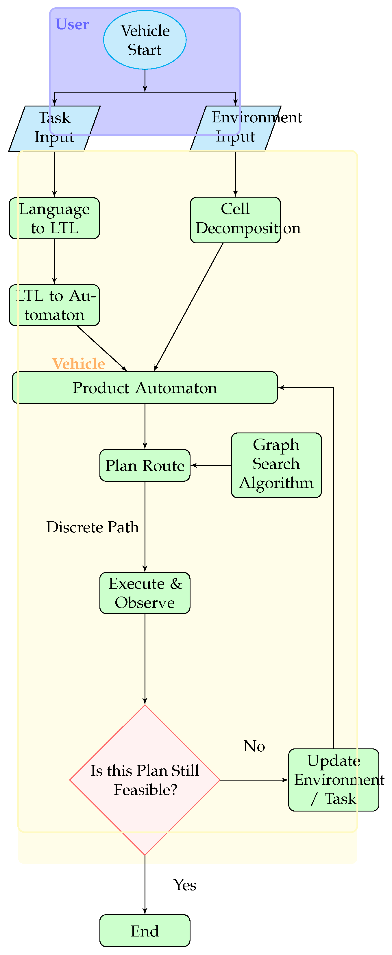
To navigate an autonomous vehicle from one location to another within a parking environment, a formal map and task specification must be provided. The task can be provided using a natural language description, which can be converted to LTL formulas using Large Language Models (LLMs). In this work, we assume that the user provides the LTL task. The task is formulated using LTL and converted into a finite automaton via tools such as SPOT [115]. Concurrently, the environment is decomposed into cells and represented as a separate automaton. These two automata, the task automaton and the environment automaton, are combined to form a product automaton that encapsulates both behavioral and spatial constraints.

Following the construction of the product automaton, a graph search algorithm such as A* or Dijkstra is applied to compute a route according to the cost function $\kappa$ defined in Equation (1). The resulting discrete path is then executed and continuously monitored. If the plan becomes infeasible due to dynamic changes in the environment or task conditions, the algorithm updates the environment and/or task and repeats the process. This iterative cycle continues until the goal is reached or a valid path becomes permanently infeasible. The complete procedural flow is illustrated in Figure 4 and described in detail in the remainder of this section.

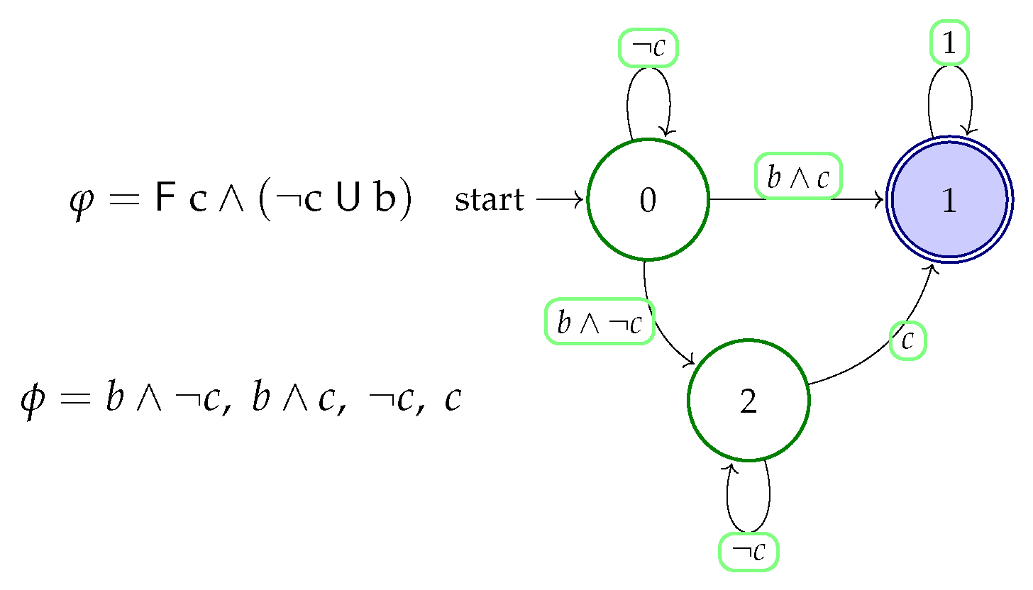
Throughout this section, we will use the example environment and the example LTL task defined in Figure 5 and Figure 6, respectively, to illustrate our key concepts.

4.1. Automaton to Matrix: A Computationally Efficient Environment and Task Representation

As mentioned in Section 2, the environment is modeled as an automaton, which is often not as efficient compared as a matrix-based representation of environments. A matrix-based representation allows efficient computation via certain matrix algebra, which significantly aids the development of our algorithm.

To that end, we first develop a connectivity matrix using the transition function ${\delta }^{\mathcal{G}}$ as follows. For a given grid environment $\mathcal{G}$ with N number of states, the connectivity matrix $M_C^{\mathcal{G}}\in {\{0,1\}}^{N\times N}$ is defined as

$$\begin{array}{c}\hfill {\left[M_C^{\mathcal{G}}\right]}_{i,j}=\left\{\begin{array}{cc}1,\hfill & \mathrm{if}\exists \sigma \in {\Sigma }^{\mathcal{G}}\mathrm{s}.\mathrm{t}.{\delta }^{\mathcal{G}}(i,\sigma )=j,\hfill \\ 0,\hfill & \mathrm{otherwise},\hfill \end{array}\right.\end{array}$$

for all states $i,j\in Q^{\mathcal{G}}$. Equivalently, $M_C^{\mathcal{G}}$ is the adjacency matrix of the directed graph underlying $\mathcal{G}$. A value of 1 at position $(i,j)$ means that from state i one can transition to state j under at least one action in ${\Sigma }^{\mathcal{G}}=\{\mathsf{u},\mathsf{d},\mathsf{l},\mathsf{r}\}$; a 0 indicates no direct transition. For example, the matrix corresponding to the 4 by 4 environment (Figure 5) would look like

Table 1. 4 by 4 Environment Matrix.

	a	c	d	b
a	1	1	0	1
c	1	1	1	0
d	0	1	1	1
b	1	0	1	1

:

Having the connectivity matrix defined, we now proceed to define the atomic proposition matrix, $M_{\pi }^{\mathcal{G}}$, for any given atomic proposition $\pi$. Recall that the Labeling function, L—as described in Section 2.2—assigns to each state $j\in Q^{\mathcal{G}}$ the set $L\left(j\right)\subseteq \Pi$ of atomic propositions true at state j. The atomic proposition matrix $M_{\pi }^{\mathcal{G}}\in {\{0,1\}}^{N\times N}$ for a proposition $\pi \in \Pi$ is constructed as follows:

For each pair of states $i,j\in Q^{\mathcal{G}}$, the $ij$-th entry of $M_{\pi }^{\mathcal{G}}$ is defined by

$${\left[M_{\pi }^{\mathcal{G}}\right]}_{i,j}={\left[M_C^{\mathcal{G}}\right]}_{i,j}\wedge {\mathbb{1}}_{[\pi \in L(j\left)\right]}$$

(2)

where ∧ denotes logical AND and ${\mathbb{1}}_{[·]}$ is the indicator function that equals 1 if $\pi$ is true at state j (i.e. $\pi \in L\left(j\right)$) and 0 otherwise. Specifically, ${\left[M_{\pi }^{\mathcal{G}}\right]}_{ij}=1$ if and only if there is an environment transition from i to j and $\pi$ holds at the destination state j. This means $M_{\pi }^{\mathcal{G}}$ retains exactly those transitions of $\mathcal{G}$ that lead into states satisfying $\pi$.

This procedure effectively filters the environment’s possible transitions, retaining only those that are compliant with a specific logical requirement. For example, one can construct matrices for atomic propositions such as $M_b^{\mathcal{G}}$ and $M_c^{\mathcal{G}}$, which will exclusively contain the environment transitions whose destination states satisfy the propositions b or c, respectively. Later, in Section 4.2.1, we will present a systematic method for constructing environment matrices corresponding to logical formulas involving multiple atomic propositions. In particular, we will illustrate the procedure with examples such as $M_{b\wedge c}$ and $M_{\neg c}$.

After defining the connectivity matrix and the atomic proposition matrix, we now proceed to define the task matrix $M^{\phi }$ obtained from the task automaton. Recall that, as mentioned at the beginning of this section, every LTL task can be converted into an automaton representation. For a given task $\phi$, let ${\mathcal{A}}^{\phi }=\{Q^{\phi },{\Sigma }^{\phi },{\delta }^{\phi },q_0^{\phi },F^{\phi }\}$ denote the automaton corresponding to the task $\phi$. For illustration, Figure 6 shows the task $\phi =\mathsf{F}\mathrm{c}\wedge (\neg \mathrm{c}\mathsf{U}\mathrm{b})$ converted into its equivalent automaton. Building on this representation, we denote its transition relation by ${\delta }^{\phi }$; specifically, ${\delta }^{\phi }(i,\varphi )=j$ if there is a transition from state $i\in Q^{\phi }$ to $j\in Q^{\phi }$ labeled by boolean formula $\varphi \in {\Sigma }^{\phi }$. As we notice, the alphabet (${\Sigma }^{\phi }$) of this automaton contains boolean functions constructed from atomic propositions. For example, for the task $\phi$ in Figure 6, the alphabet consists of $\{\neg c,b\wedge c,b\wedge \neg c,c\}$ where $b,c\in \Pi$. Formally stated, the alphabet ${\Sigma }^{\phi }$ of the task automaton ${\mathcal{A}}^{\phi }$ is the set of all Boolean formulas that can be constructed from the atomic propositions. Formally, for all states $i,j\in Q^{\phi }$, the task matrix is defined as:

$$\begin{array}{c}\hfill {\left[M^{\phi }\right]}_{i,j}=\left\{\begin{array}{cc}\varphi ,\hfill & \mathrm{if}{\delta }^{\phi }(i,\varphi )=j,\hfill \\ 1,\hfill & \mathrm{if}{\delta }^{\phi }(i,true)=j,\hfill \\ 0,\hfill & \mathrm{otherwise}.\hfill \end{array}\right.\end{array}$$

Each entry ${\left[M^{\phi }\right]}_{i,j}$ in the task matrix encodes the condition under which a transition from task automaton state i to j is allowed. The matrix is defined as follows:

• If there exists a transition ${\delta }^{\phi }(i,\varphi )=j$, where $\varphi$ is a logical formula over atomic propositions (e.g., $\neg c$, $b\wedge c$), then ${\left[M^{\phi }\right]}_{i,j}=\varphi$. This includes conditional self-loops when $i=j$.
• If there exists an unconditional self-loop, i.e., ${\delta }^{\phi }(i,true)=j$, then ${\left[M^{\phi }\right]}_{i,i}=1$. This indicates a transition that is always enabled.
• If no transition from i to j is defined in the task automaton, then ${\left[M^{\phi }\right]}_{i,j}=0$.

For instance, for task $\mathsf{F}\mathrm{c}\wedge (\neg \mathrm{c}\mathsf{U}\mathrm{b})$ described in Figure 6 results in the

Table 2. Task Matrix.

	0	1	2
0	$\neg c$	$b\wedge c$	$b\wedge \neg c$
1	0	1	0
2	0	c	$\neg c$

:

This construction formalizes how the task automaton encodes logical constraints on transitions and sets the stage for integrating it with the environment model during product automaton synthesis.

4.2. Product Automaton Matrix: Matrix Fusion for Integrated Planning

Following the definition of the environment connectivity matrix ($M_C^{\mathcal{G}}$) and the task automaton matrix, the next step is to combine them into a single structure suitable for integrated planning. This is achieved by constructing a product automaton matrix, which fuses the physical pathways of the environment with the logical constraints imposed by the task. This process is a crucial part of creating the product automaton shown in the overall system flowchart (Figure 4). Each transition in the task automaton is labeled with a Boolean formula, $\varphi$ (e.g., $\neg c$, $b\wedge c$, $b\wedge \neg c$, or c, etc. in Figure 6), which dictates the conditions required for that transition. These formulas appear as entries in the task matrix, $M^{\phi }$ (see Table 2), i.e., ${\left[M^{\phi }\right]}_{ij}$’s. To embed these rules into the environment, we already generated an atomic proposition matrix, $M_{\pi }^{\mathcal{G}}$ (Equation (2)), for each logical formula.

4.2.1. Boolean Operations on Atomic Matrices (For Formulas)

We now formalize the construction of the constraint matrix $M_{\varphi }^{\mathcal{G}}$ for any arbitrary Boolean formula $\varphi$. While the previous section demonstrated how to construct matrices for atomic propositions (e.g., $M_b^{\mathcal{G}}$ and $M_c^{\mathcal{G}}$; see Equation (2)), this section provides a recursive grammar that generalizes the method to all complex formulas built from these atoms. This ensures a systematic and computationally sound approach for embedding any logical task requirement into the environment matrix. Formally:

$$\begin{array}{cc}\hfill M_{\neg \varphi }^{\mathcal{G}}& =M_C^{\mathcal{G}}\wedge (\neg M_{\varphi }^{\mathcal{G}}),\hfill \end{array}$$

(3)

$$\begin{array}{cc}\hfill M_{{\varphi }_1\wedge {\varphi }_2}^{\mathcal{G}}& =M_{{\varphi }_1}^{\mathcal{G}}\wedge M_{{\varphi }_2}^{\mathcal{G}},\hfill \end{array}$$

(4)

$$\begin{array}{cc}\hfill M_{{\varphi }_1\vee {\varphi }_2}^{\mathcal{G}}& =M_{{\varphi }_1}^{\mathcal{G}}\vee M_{{\varphi }_2}^{\mathcal{G}}.\hfill \end{array}$$

(5)

The operators on the right-hand side represent element-wise logical operations:

• Conjunction (∧) and Disjunction (∨): These operations are performed as direct element-wise AND and OR on the operand matrices. For instance, ${\left[M_{{\varphi }_1\wedge {\varphi }_2}^{\mathcal{G}}\right]}_{ij}={\left[M_{{\varphi }_1}^{\mathcal{G}}\right]}_{ij}\wedge {\left[M_{{\varphi }_2}^{\mathcal{G}}\right]}_{ij}$. Because the base matrices are already filtered by the environment connectivity, the results of these operations are inherently valid paths.
• Negation (¬): The negation of a formula, $\neg \varphi$, represents all valid environment transitions where the condition $\varphi$ is not met. This is calculated by taking the element-wise complement of $M_{\varphi }^{\mathcal{G}}$ (which marks transitions where $\varphi$ is false) and then performing an element-wise AND with the environment connectivity matrix $M_C^{\mathcal{G}}$. This final AND operation ensures that the resulting matrix $M_{\neg \varphi }^{\mathcal{G}}$ only contains transitions that are physically possible in the environment.

This grammar provides a rigorous and scalable method for translating any task-level Boolean formula into a corresponding constraint matrix, directly embedding the logical requirements of the plan into the state-space of the environment.

To provide a concrete example of this grammar, let us apply Equation (4) to compute the constraint matrix for the formula $\varphi =b\wedge c$. We start with the atomic proposition matrices for b and c, which (based on our 4-state environment) are:

$$M_b^{\mathcal{G}}=\left[\begin{array}{cccc}0& 0& 0& 1\\ 0& 0& 0& 0\\ 0& 0& 0& 1\\ 0& 0& 0& 1\end{array}\right]M_c^{\mathcal{G}}=\left[\begin{array}{cccc}0& 1& 0& 0\\ 0& 1& 0& 0\\ 0& 1& 0& 0\\ 0& 0& 0& 0\end{array}\right].$$

The conjunction $M_{b\wedge c}^{\mathcal{G}}=M_b^{\mathcal{G}}\wedge M_c^{\mathcal{G}}$ is computed by applying an element-wise logical AND operation. This operation yields a 1 in an entry $(i,j)$ only if the entry is 1 in both $M_b^{\mathcal{G}}$ and $M_c^{\mathcal{G}}$. In this case, no single entry $(i,j)$ meets this condition. For instance, while $M_b^{\mathcal{G}}(a,b)=1$, $M_c^{\mathcal{G}}(a,b)=0$, so $(a,b)$ is 0 in the result. The resulting matrix is:

$$M_{b\wedge c}^{\mathcal{G}}=\left[\begin{array}{cccc}0& 0& 0& 0\\ 0& 0& 0& 0\\ 0& 0& 0& 0\\ 0& 0& 0& 0\end{array}\right].$$

This resultant matrix $M_{b\wedge c}^{\mathcal{G}}$ correctly identifies that there are no valid transitions in the environment that simultaneously satisfy both propositions b and c.

Remark 1

(Computational Efficiency of the Matrix-Based Approach). The grammatical approach to constructing constraint matrices offers significant computational advantages, particularly for systems with large state spaces or complex logical specifications. The primary source of this efficiency lies in a “compute-once, reuse-many” paradigm.

The most computationally intensive step is the initial evaluation of state transition conditions against the environment model. Our method isolates this task by performing it only once; once these foundational matrices are pre-computed, the matrix for any arbitrarily complex compound formula ϕ can be derived through a series of highly optimized, element-wise Boolean operations.

To illustrate, consider a naive approach where the matrix for a formula like $\varphi =({\varphi }_1\wedge {\varphi }_2)\vee \neg {\varphi }_3$ would be computed by re-evaluating the underlying conditions for ${\varphi }_1$, ${\varphi }_2$, and ${\varphi }_3$ across all state transitions. In contrast, our matrix-based method avoids this redundant processing entirely. It simply reuses the existing matrices $M_{{\varphi }_1}^{\mathcal{G}}$, $M_{{\varphi }_2}^{\mathcal{G}}$, and $M_{{\varphi }_3}^{\mathcal{G}}$ and computes the final matrix $M_{\varphi }^{\mathcal{G}}$ with inexpensive logical operations. This elimination of redundant computation makes the synthesis of complex constraint matrices highly scalable and efficient.

4.2.2. Building Product Automaton Matrix

To build the product automaton matrix, we substitute each logical formula $\varphi$ in the task matrix with the corresponding environment matrix $M_{\varphi }^{\mathcal{G}}$. The result is a block-structured adjacency matrix for the product, representing all combinations of task states and environment states. This composite matrix has dimensions $\left(N^{\phi }{N}^{\mathcal{G}}\right)\times \left(N^{\phi }{N}^{\mathcal{G}}\right)$, where $N^{\phi }=\left|Q^{\phi }\right|$ is the number of states in the task automaton and $N^{\mathcal{G}}$ is defined analogously for the environment automaton. Within this matrix, an entry corresponding to $((i^{\mathcal{G}},i^{\phi })\to (j^{\mathcal{G}},j^{\phi }))$ is 1 if and only if the environment allows $i^{\mathcal{G}}\to j^{\mathcal{G}}$ and the task formula on $i^{\phi }\to j^{\phi }$ is satisfied. In other words, a transition in the product automaton is enabled only when both spatial feasibility (from the environment) and logical validity (from the task) conditions hold simultaneously. More formally, the following conditions are hold:

• $\exists \sigma \in {\Sigma }^{\mathcal{G}}$ such that ${\delta }^{\mathcal{G}}(i^{\mathcal{G}},\sigma )=j^{\mathcal{G}}$, and
• ${\delta }^{\phi }(i^{\phi },L\left(j^{\mathcal{G}}\right))=j^{\phi }$.

4.2.3. Formalizing the Product via Conditional Block Operator

We introduce a novel binary operator, denoted by $\begin{array}{|c|}\hline \varphi \\ \hline\end{array}$ and referred to as the Conditional Block Product, which combines a base matrix $M^1$ with a label matrix $M^2$ to yield a structured block matrix. Let $M^1\in {\mathbb{R}}^{m\times n}$ and $M^2\in {\Lambda }^{p\times q}$, where $\Lambda$ denotes the set containing 0, 1, and logical formulas constructed from a fixed set of atomic propositions. The result is a Product Automaton matrix ($M^3$) of size $\left(pm\right)\times \left(qn\right)$, partitioned into $p\times q$ blocks of dimension $m\times n$:

$$M^1\begin{array}{|c|}\hline \varphi \\ \hline\end{array}{M}^2=M^3.$$

(6)

Each block $(i,j)$ in the output matrix $M^3$ is defined as follows:

• If ${\left[M^2\right]}_{i,j}=0$, the corresponding block is the $m\times n$ zero matrix.
• If ${\left[M^2\right]}_{i,j}=1$, the block is assigned the matrix $M^1$.
• If ${\left[M^2\right]}_{i,j}=\varphi$ is a logical formula, the block is also set to $M_{\varphi }^1$ (under the condition $\varphi$), where $M_{\varphi }^1$ computed using Equations (3)–(5).

Formally, the operator maps each entry of the label matrix to a block: non-zero entries (logical or Boolean) yield copies of $M^1$ or $M_{\varphi }^1$, while zero entries yield zero matrices. This operator generalizes structured matrix expansion based on symbolic logic and provides a flexible mechanism for constructing labeled matrix products. In our example (Table 1 and Table 2) $M_C^{\mathcal{G}}\in {\{0,1\}}^{4\times 4}$ and

$$\begin{array}{c}\hfill M^{\phi }=\left[\begin{array}{ccc}\neg c& b\wedge c& b\wedge \neg c\\ \mathbf{0}& 1& \mathbf{0}\\ \mathbf{0}& c& \neg c\end{array}\right].\end{array}$$

where b, c, and $\neg c$ are logical conditions. Then, $M_C^{\mathcal{G}}\begin{array}{|c|}\hline \varphi \\ \hline\end{array}{M}^{\phi }$ is a $12\times 12$ matrix (

Table 3. Product Automaton Matrix.

		Future State
		0a	0c	0d	0b	1a	1c	1d	1b	2a	2c	2d	2b
Present State	0a	1	0	0	1	0	0	0	0	0	0	0	1
	0c	1	0	1	0	0	0	0	0	0	0	0	0
	0d	0	0	1	1	0	0	0	0	0	0	0	1
	0b	1	0	1	1	0	0	0	0	0	0	0	1
	1a	0	0	0	0	1	1	0	1	0	0	0	0
	1c	0	0	0	0	1	1	1	0	0	0	0	0
	1d	0	0	0	0	0	1	1	1	0	0	0	0
	1b	0	0	0	0	1	0	1	1	0	0	0	0
	2a	0	0	0	0	0	1	0	0	1	0	0	1
	2c	0	0	0	0	0	1	0	0	1	0	1	0
	2d	0	0	0	0	0	0	0	0	0	0	1	1
	2b	0	0	0	0	0	0	0	0	1	0	1	1

) consisting of the following blocks:

$$\begin{array}{c}\hfill \left[\begin{array}{ccc}{M}_{\neg c}^{\mathcal{G}}& M_{b\wedge c}^{\mathcal{G}}& M_{b\wedge \neg c}^{\mathcal{G}}\\ \mathbf{0}& M_C^{\mathcal{G}}& \mathbf{0}\\ \mathbf{0}& M_c^{\mathcal{G}}& M_{\neg c}^{\mathcal{G}}\end{array}\right].\end{array}$$

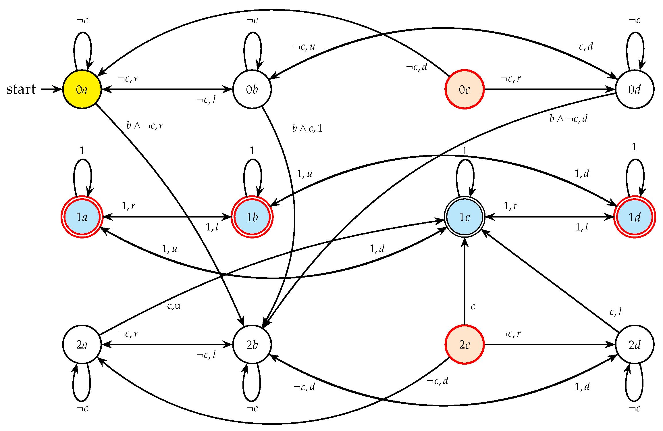
Note that some blocks in this matrix are conditioned on logical formulas. The product automaton according to Table 3 has been shown in Figure 7, where 0a is the starting state (colored by Yellow) and 1a, 1b, 1c, 1d are accepted states colored by blue. Appendix A provides additional details on constructing and validating the product automaton.

This approach remains general and adaptable: updates to the environment connectivity or task logic can be localized to the corresponding environment matrix or task automaton matrix. Once updated, the product automaton matrix can be efficiently reconstructed using the defined conditional-block-product operation, ensuring consistent integration of both physical and logical constraints.

Remark 2

(Motion Cost Encoding in Product Automaton Space). In the product automaton matrix $M^{\mathcal{P}}$, constructed from the environment connectivity matrix $M_C^{\mathcal{G}}$ representing spatial transitions and the task matrix $M^{\phi }$ of atomic propositions encoding logical constraints derived from an LTL specification, each non-zero entry represents a valid transition that satisfies both spatial and logical constraints. The cost associated with transitioning from a product state $(q_n^{\mathcal{G}},q_n^{\phi })$ to another product state $({q\prime }_n^{\mathcal{G}},{q\prime }_n^{\phi })$ directly inherits its transition cost from the underlying environment transition $q_n^{\mathcal{G}}\stackrel{\sigma }{\to }{q\prime }_n^{\mathcal{G}}$. This cost is determined by the environment’s transition cost function κ (introduced in Equation (1)). Specifically, the cost matrix for the product automaton, $C^{\mathcal{P}}$, is constructed by assigning the cost $\kappa (q_n^{\mathcal{G}},\sigma )$ to the entry in $C^{\mathcal{P}}$ corresponding to the valid product transition from $(q_n^{\mathcal{G}},q_n^{\phi })$ to $({q\prime }_n^{\mathcal{G}},{q\prime }_n^{\phi })$, where σ is the action that enables the transition $q_n^{\mathcal{G}}\stackrel{\sigma }{\to }{q\prime }_n^{\mathcal{G}}$.

This modeling naturally forms a Weighted Transition System (WTS), where κ assigns weights to transitions, and optimal paths minimize the total transition cost. This cost assignment ensures that the product automaton accurately represents both spatial and behavioral constraints within a unified weighted transition framework. Consequently, shortest-path algorithms such as Dijkstra’s algorithm may utilize this cost matrix to compute optimal paths.

4.3. Pruning of Product Automaton Matrix

To create a minimal and efficient automaton, the state space of the product automaton is optimized by pruning redundant states. A state is identified as redundant and removed if it meets any of the following three criteria.

Pruning Rule 1. Unreachable State Elimination (Column-wise Pruning): For each state $j_n$, if column $j_n$ of the product matrix $M^{\mathcal{P}}$ is a zero vector (i.e., $\forall i:{\left[M^{\mathcal{P}}\right]}_{i,j_n}=0$), then state $j_n$ is unreachable and should be removed. When pruning such a state, eliminate its column $j_n$ from $M^{\mathcal{P}}$ and also remove the corresponding row $j_n$ (the same state’s row in the matrix).

Pruning Rule 2. Redundant Accepting-State Pruning: If state $j_n$ is accepting ($j_n\in N_{\mathit{acc}}$ [here, $N_{\mathit{acc}}$ is set of accepted states]) and all incoming transitions to $j_n$ originate from other accepting states (i.e., $\forall i:{\left[M^{\mathcal{P}}\right]}_{i,j_n}=1$ implies $i\in N_{\mathit{acc}}$), then column $j_n$ and its corresponding row $j_n$ are redundant and can be eliminated. To compute $N_{acc}$, take the accepting set of the product automaton:

$$N_{acc}=F_{acc}=F^{{\mathcal{A}}^{\mathcal{G}}}\times F^{{\mathcal{A}}^{\phi }}.$$

Pruning Rule 3. Deadlock-State Elimination (Row-wise Pruning): For any state $i_n$, if its row in $M^{\mathcal{P}}$ has zeros in every column except the diagonal (i.e., ${\left[M^{\mathcal{P}}\right]}_{i_n,i_n}=1$ and $\forall j\ne i_n:{\left[M^{\mathcal{P}}\right]}_{i_n,j}=0$), then state $i_n$ is a self-loop (deadlock) state. Such a non-accepting state cannot reach any other state and is prunable.

Each rule is applied iteratively to the product automaton’s transition matrix to remove superfluous states. The result is a reduced automaton that preserves all reachable behavior relevant to the specification.

In practice, Rule 1 identifies states with no predecessors. For example,

Table 4. Product Automaton Matrix (Pruning Process). The state labels are color-coded by their properties: yellow indicates the initial state; blue indicates the set of accepting states; orange with a red border denotes states pruned by Rule-1 (column-wise); and blue with a red border denotes states pruned by Rule-2 (Redundant Accepting-state pruning).

		Future State
		0a		0d	0b					2a		2d	2b
Present State		1	0	0	1	0	0	0	0	0	0	0	1
		1	0	1	0	0	0	0	0	0	0	0	0
	0d	0	0	1	1	0	0	0	0	0	0	0	1
	0b	1	0	1	1	0	0	0	0	0	0	0	1
		0	0	0	0	1	1	0	1	0	0	0	0
		0	0	0	0	1	1	1	0	0	0	0	0
		0	0	0	0	0	1	1	1	0	0	0	0
		0	0	0	0	1	0	1	1	0	0	0	0
	2a	0	0	0	0	0	1	0	0	1	0	0	1
		0	0	0	0	0	1	0	0	1	0	1	0
	2d	0	0	0	0	0	0	0	0	0	0	1	1
	2b	0	0	0	0	0	0	0	0	1	0	1	1

(the original product automaton matrix) shows that the columns for states “0c” and “2c”—highlighted with red outlines—are entirely zero, meaning states 0c and 2c colored by orange in both Table 4 and Figure 7) have no incoming transitions. According to Rule 1, these states are unreachable and are removed. Pruning such unreachable states is standard in automaton minimization. Eliminating them ensures that the remaining matrix contains only states reachable from the start.

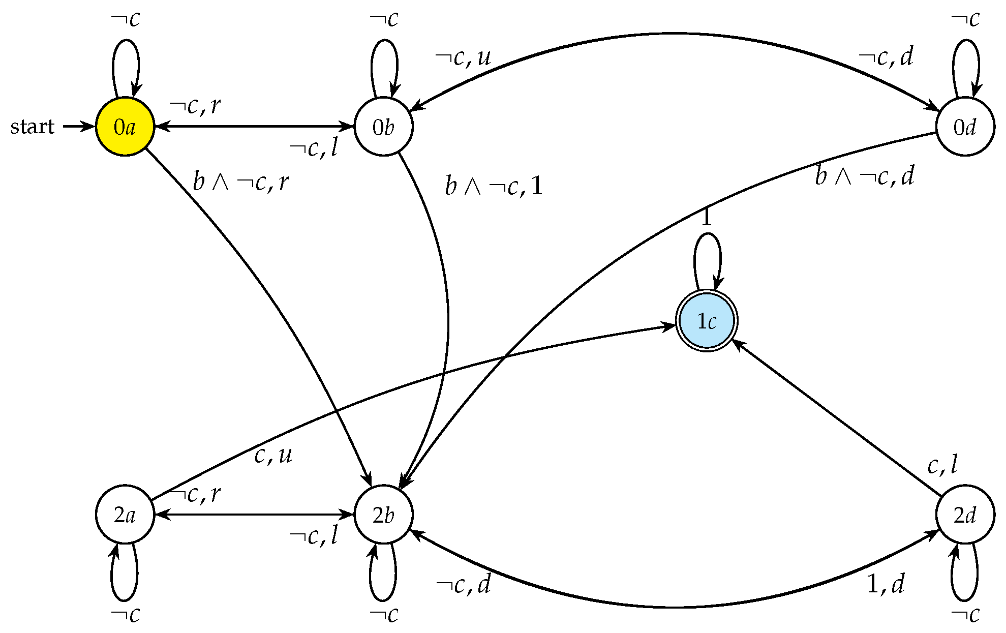
Rule 2 prunes accepting states that form a closed accepting subgraph, i.e., states whose incoming transitions all originate from accepting states. Since they introduce no paths to non-accepting states, removing these states and their outgoing edges does not change the accepted run. In Table 4, states 1a, 1d, and 1b meet this criterion (red outlines). The final pruned matrix has been shown in

Table 5. Pruned product Automaton Matrix.

		Future State
		0a	0d	0b	1c	2a	2d	2b
Present State	0a	1	0	1	0	0	0	1
	0d	0	1	1	0	0	1	1
	0b	1	1	1	0	0	0	1
	1c	0	0	0	1	0	0	0
	2a	0	0	0	1	1	0	1
	2d	0	0	0	0	0	1	1
	2b	0	0	0	0	1	1	1

and the pruned product automaton itself shown in Figure 8.

Rule 3 applies to an uncontrollable or deadlock condition, meaning once the automaton enters this state, it cannot transition to any other state. Consequently, if this state is not an accepting state, it is effectively redundant and should be eliminated to achieve a minimal and efficient automaton structure. In the current example, none of the states satisfy this rule. We can examine Figure 7 for illustration. States like 2a and 2b possess self-loops but also have transitions to other states (2b and 2d, respectively), so they are not true deadlock states under this definition. A state would be pruned by Rule 3 if it were a non-accepting state with only a self-loop (or no outgoing transitions at all), as it would represent a terminal, non-accepting condition.

The final, reduced product automaton matrix, containing only the essential states after applying these pruning procedures, is illustrated in Table 5.

4.4. Path Planning in Product Automaton Matrix

The Algorithm 1 begins by converting the high-level task specified in LTL into an equivalent finite-state automaton that captures the desired temporal behavior. Next, this automaton is synchronized with a weighted transition model of the environment (a graph of allowable moves and costs) to form a product automaton that encodes both the mission goals and the operational constraints. Once, the product automaton matrix is constructed, path planning becomes a graph search problem: the objective is to find a valid path starting from the initial product state $(q_0^{\mathcal{G}},q_0^{\phi })$ and ending at any accepting product state $(q_n^{\mathcal{G}},q_n^{\phi })$.

Algorithm 1: Path Planning with LTL Constraint
Input: Environment Connectivity Matrix $M_C^{\mathcal{G}}\in {\{0,1\}}^{N\times N}$, LTL Task $\phi$, Car Location $v_0\in \mathcal{N}$ Output: Final Path ${\mathbb{P}}_f$
1 $M^{\phi }\leftarrow \mathrm{LTL}2\mathrm{Matrix}\left(\phi \right)$; 2 $M^P\leftarrow \mathrm{ProductAutomatonMatrix}(M^{\phi },M_C^{\mathcal{G}})$ 3 $\widehat{M^P}\leftarrow \mathrm{Prune}\left(M^P\right)$ 4 $W_{\mathcal{G},\phi }\leftarrow \mathrm{WTS}\left(\widehat{M^P}\right)$; 5 ${\xi }_0\leftarrow (v_0,{\tau }_0)$; 6 $F\leftarrow \{(v,{\tau }_f):v\in F_{acc},{\tau }_f\in F^{{\mathcal{A}}^{\phi }}\}$ 7 ${\Pi }_f\leftarrow$PathPlanning$\left({\xi }_0,F\right)$ 8 ${\mathbb{P}}_f\leftarrow \mathrm{Project}\left({\Pi }_f\right)$	//Using available tool SPOT // Equation (6) //Remark 2 //${\tau }_0=q_0^{{\mathcal{A}}^{\phi }}$ (initial state of ${\mathcal{A}}^{\phi }$)$\phantom{(}$

Multiple such accepting states may exist. A valid path in the product space can be defined as a sequence of transitions:

$$(q_0^{\mathcal{G}},q_0^{\phi })\to (q_1^{\mathcal{G}},q_1^{\phi })\to \cdots \to (q_n^{\mathcal{G}},q_n^{\phi }),$$

(7)

Each product transition thus captures both a feasible physical move and a logically valid automaton progression. Therefore, planning in the product automaton reduces to finding a path from the initial product state to any accepting product state using standard graph search algorithms (e.g., Dijkstra’s, A*). Finally, because the goal is to execute the motion in the environment, the projection operation maps the product-space path in Equation (7) back to the original state space, producing the environment path $q_0^{\mathcal{G}}\to q_1^{\mathcal{G}}\to \cdots \to q_n^{\mathcal{G}}$ with the same accumulated cost. A valid example path in the constructed automaton (Table 4) is $\left(0a\right)\to \left(2b\right)\to \left(2a\right)\to \left(1c\right)$, where, the initial product state (yellow colored) is $\left(0a\right)$ and one of the accepting product state (blue colored) is $\left(1c\right)$. The first transition $\left(0a\right)$ to $\left(2b\right)$ signifies moving from cell “a” to “b” in the environment and from state 0 to 2 in the task automaton, adhering to the proposition $b\wedge \neg c$. Some generated trajectories have been shown in Section 5. This pipeline yields a trajectory that minimizes travel cost while rigorously satisfying the complex LTL specification, a combination ideally suited to mission-critical autonomous navigation.

While Algorithm 1 provides the high-level workflow, the specific algorithmic details for its core components are defined in the preceding sections. The formal procedure for the ProductAutomatonMatrix (Line 2) is detailed in Section 4.2.2 (Equation (4)). The Prune function (Line 3) is based on the three pruning rules detailed in Section 4.3. The WTS function (Line 4) applies the formal cost derivation from Equation (1) and Remark 2, and the PATHPLANNING function (Line 7) is an implementation of a standard complete graph search algorithm, such as Dijkstra’s.

5. Results & Discussions

A set of parking-lot environments was used across the experiments, with scale chosen to match each objective. Experiments 1–3 use the same compact, grid-based lot to isolate effects of task changes, traffic-rule enforcement, and goal replanning. Experiment 4 moves to a medium-size 17 × 8 layout, and Experiment 5 stress-tests scalability in a large 28 × 35 facility selected specifically for robustness and mission-planning evaluation. Experiment 6 then utilizes this same large-scale environment to benchmark computational performance, specifically comparing the replanning efficiency of our matrix-based method against the traditional automata-based approach. Across all environments, the lot includes marked parking stalls, entry/exit gates, one-way traffic lanes (yellow arrows), and static elements such as parked vehicles, reserved spots, and traffic signs (e.g., no-entry/restricted parking). In each experiment, the ego vehicle (red) starts from a designated entry and is guided by the SPTL planner to reach its target while respecting the applicable constraints of that scenario.

The six experiments conducted within this environment are summarized as follows:

• Experiment 1: Shortest-path planning with a change in task requirements.
• Experiment 2: Introduction of one-way traffic rules and a dynamic obstacle, testing rule enforcement and replanning.
• Experiment 3: Dynamic goal change mid-mission due to a road blockage, evaluating the agility of the planner.
• Experiment 4: Smart parking with real-time slot updates and dynamic goal reassignment.
• Experiment 5: Multi-stage autonomous mission integrating drop-off, pick-up, task cancellation, and obstacle avoidance in a large-scale parking environment.
• Experiment 6: A computational benchmark comparing the Product Automaton generation time of the proposed matrix-based method against a traditional iterative, automata-theoretic approach during a dynamic task change.

5.1. Experiment 1: Shortest-Path Planning with Task Modifications

The routing results for Experiment 1 are illustrated in Figure 9. In Case 1 (Figure 9a), the ego vehicle follows the shortest path from the entry point to the original exit goal. The SPTL algorithm computes a direct route that satisfies the task. In Case 2 (Figure 9b), the task specification is modified to include an intermediate pickup point. As a result, the planned path detours to the pickup location before proceeding to the exit, demonstrating the planner’s ability to incorporate sequential tasks. In Case 3 (Figure 9c), a static obstacle is introduced on the initially planned route. This blockage causes the original path to be infeasible, so the planner dynamically replans an alternate path around the obstruction. The new trajectory still satisfies the task (including the pickup) while avoiding the obstacle, illustrating the system’s replanning capability under LTL task constraints.

Experiment 1 primarily validated algorithmic correctness and logical task satisfaction under sequential and obstructed navigation conditions. Therefore, timing metrics were not collected. However, qualitative observations confirmed smooth trajectory reconstruction and consistent path feasibility across all test cases.

5.2. Experiment 2: Traffic Rules and Dynamic Obstacle Handling

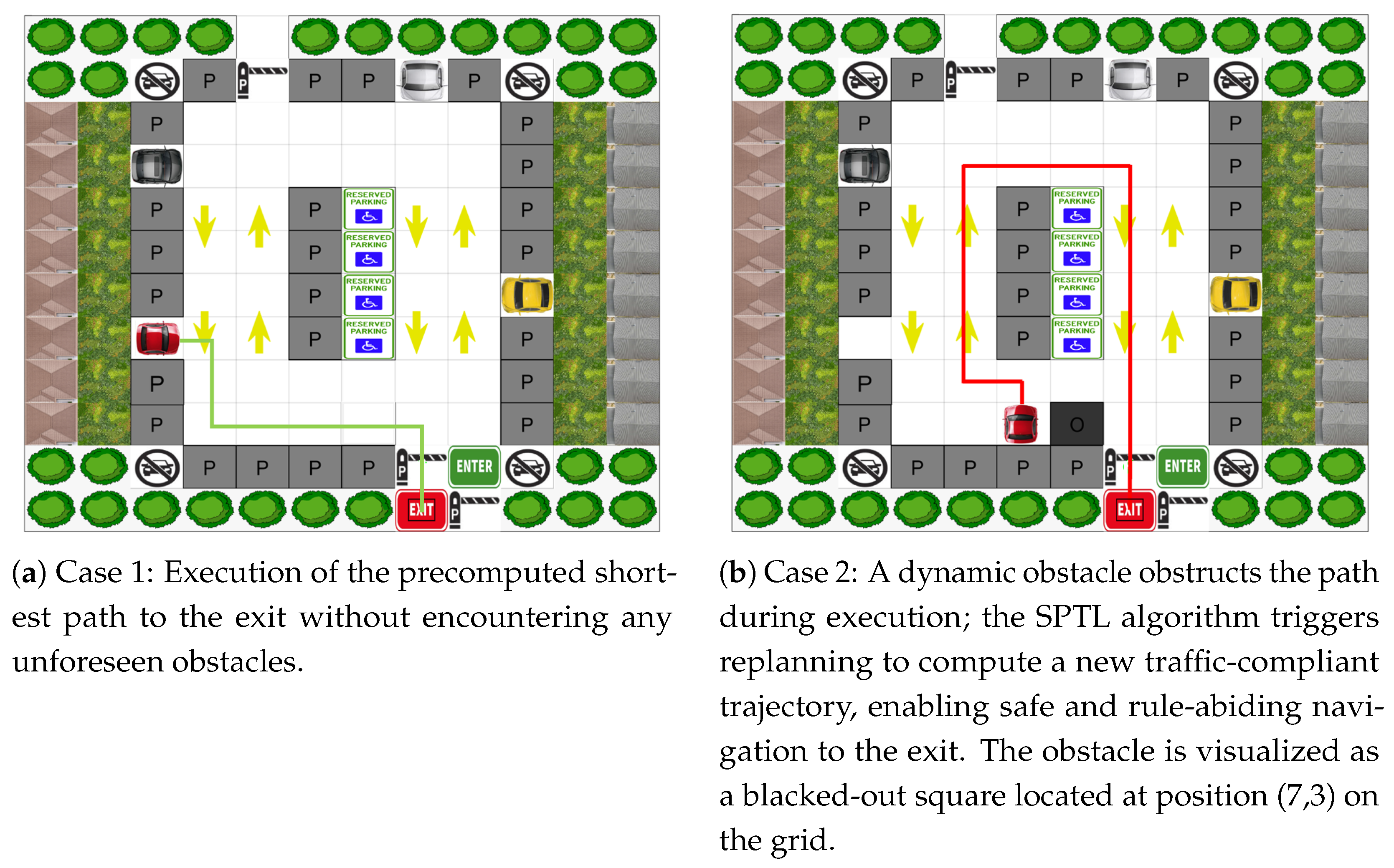
Experiment 2 (Figure 10) incorporates traffic rules by modifying the automaton to enforce one-way flow along the yellow-lane directions. In Case 1 (Figure 10a), the planned path in green strictly follows the designated arrows and avoids illegal turns; the ego vehicle travels along permitted lanes to reach its goal. This differs from Experiment 1, where such traffic constraints were not applied.

In Case 2 (Figure 10b), a pedestrian/obstacle (visualized in black) suddenly appears on the lane. The SPTL planner detects the obstacle and triggers replanning: it recomputes a new route that still respects the one-way rules. The result is a longer path that circumvents the blockage, demonstrating successful integration of dynamic replanning with traffic-rule compliance.

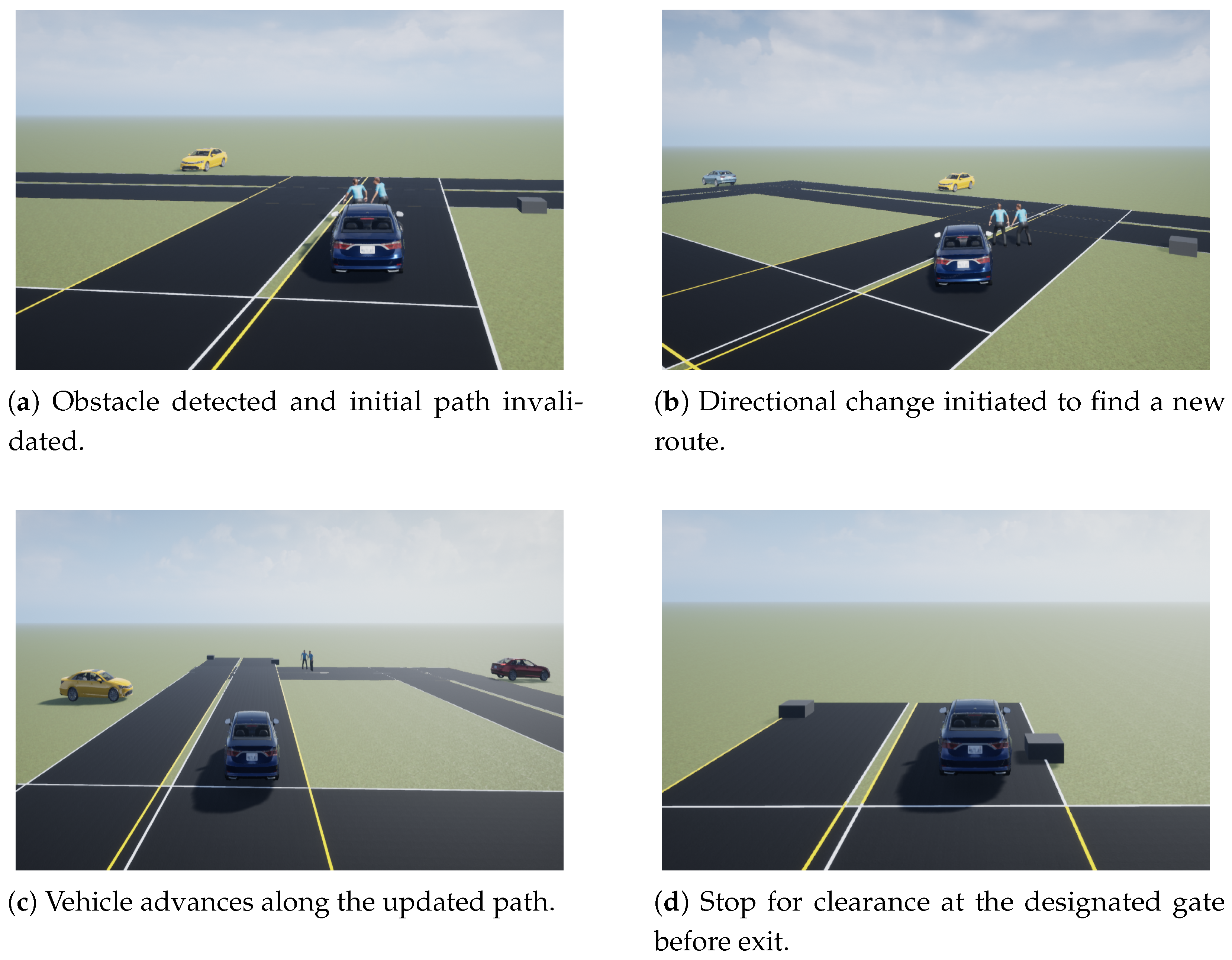
The simulation is further validated in a high-fidelity Driving Scenario Designer environment (Figure 11). Here, the computed trajectory is deployed on a realistic vehicle model (blue vehicle) in a 3D scene. The vehicle moves along the planned route toward the exit, with other traffic participants (yellow and red vehicles) present in the scene. When two pedestrians suddenly come in front of the vehicle (Figure 11a), it replans it’s path and goes to the exit. The vehicle comes to a safe stop at the exit gate when an obstacle is detected, ensuring clearance (Figure 11d). These results highlight that the SPTL-generated path can be executed on a realistic platform while maintaining obstacle avoidance and adherence to traffic rules.

Across 25 simulation runs, the mean total computation time was $0.5061\pm 0.0442$ s. The mean initial Product Automaton (PA) generation time was $0.4152\pm 0.0345$ s. The planner computed the first path segment before replanning in $0.0137\pm 0.0009$ s, while recomputation of the path after replanning was completed in $0.0023\pm 0.0020$ s. The PA rebuild during replanning took only $0.0077\pm 0.0012$ s. All metrics exhibited low variance across trials, confirming consistent real-time performance. The planner successfully executed dynamic obstacle handling and rule-compliant trajectory adaptation within milliseconds, validating the framework’s robustness, computational efficiency, and suitability for constrained traffic environments.

5.3. Experiment 3: Dynamic Goal Change and Replanning

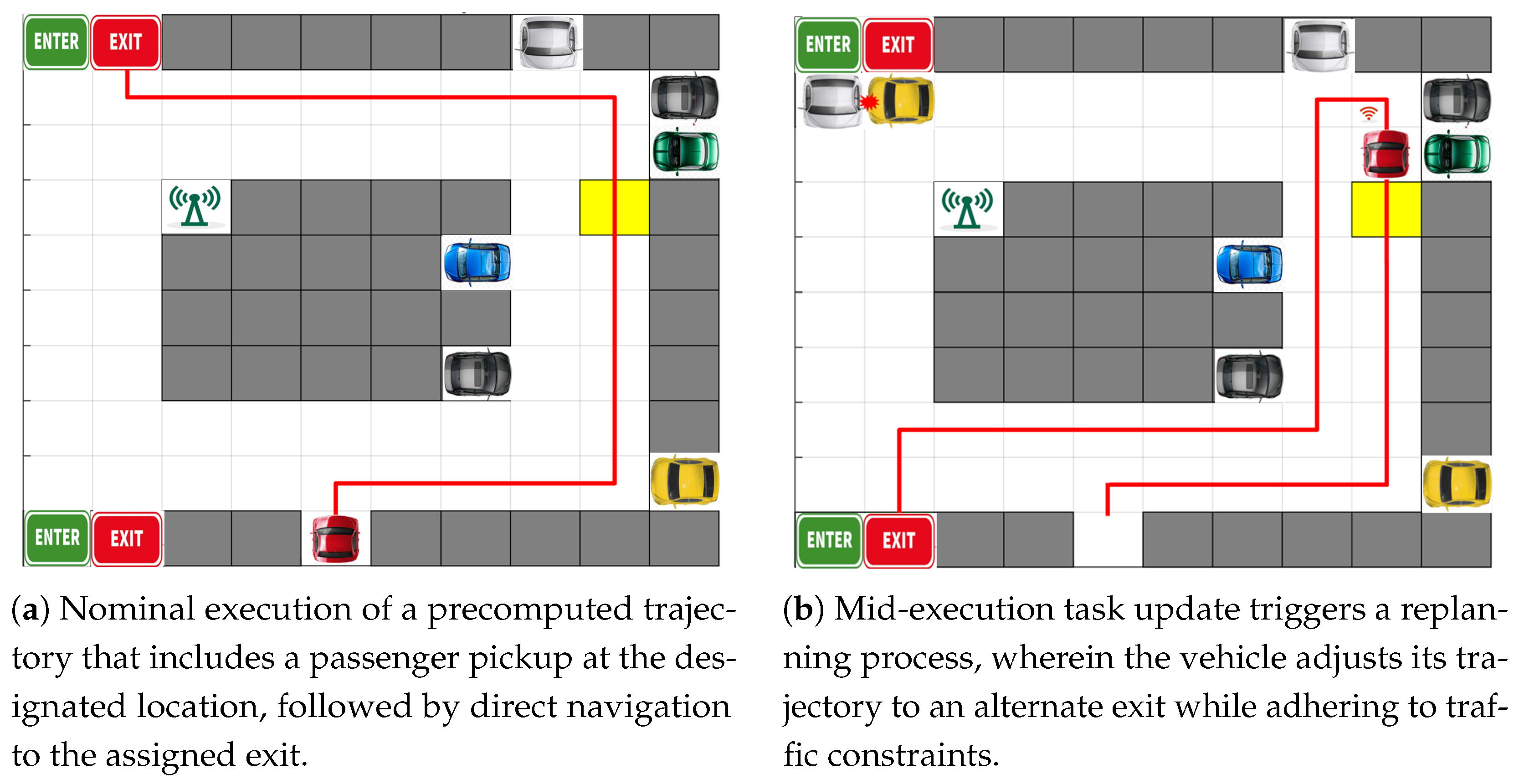
Experiment 3 demonstrates goal change and replanning. The scenario begins with the ego vehicle navigating toward an initial goal. In Case 1 (Figure 12a), the vehicle follows the planned path to the first goal as expected after picking up something from the yellow region. In Case 2 (Figure 12b), during execution, a road blockage is reported (indicated by the sensor symbol) that renders the original exit unreachable. In response, the task goal is changed dynamically after the pickup point. The planner immediately computes a new path to the updated goal. The resulting trajectory (red) guides the vehicle from its current location to the alternate exit, still respecting the traffic directionality constraints. These results demonstrate the system’s agility: it can re-synthesize a correct trajectory in real time when the goal changes, while continuing to obey the traffic rules.

The mean total computation time was $0.5231\pm 0.0886$ s, and the average replanning latency was $0.335\pm 0.011$ s. The initial PA generation required $0.4311\pm 0.0864$ s. Additionally, the planner computed the first path segment before replanning in $0.0136\pm 0.0007$ s and recomputed the updated path after replanning in just $0.0029\pm 0.0004$ s. The PA rebuild during replanning took only $0.0078\pm 0.0009$ s. Despite the increased complexity from mid-mission goal changes, the low variance across all metrics highlights the framework’s consistency and responsiveness. These findings reinforce the system’s agility and temporal stability, showing that it can seamlessly adapt to evolving mission objectives in real time while ensuring rule compliance.

5.4. Experiment 4: Smart Parking with Dynamic Goal Reassignment

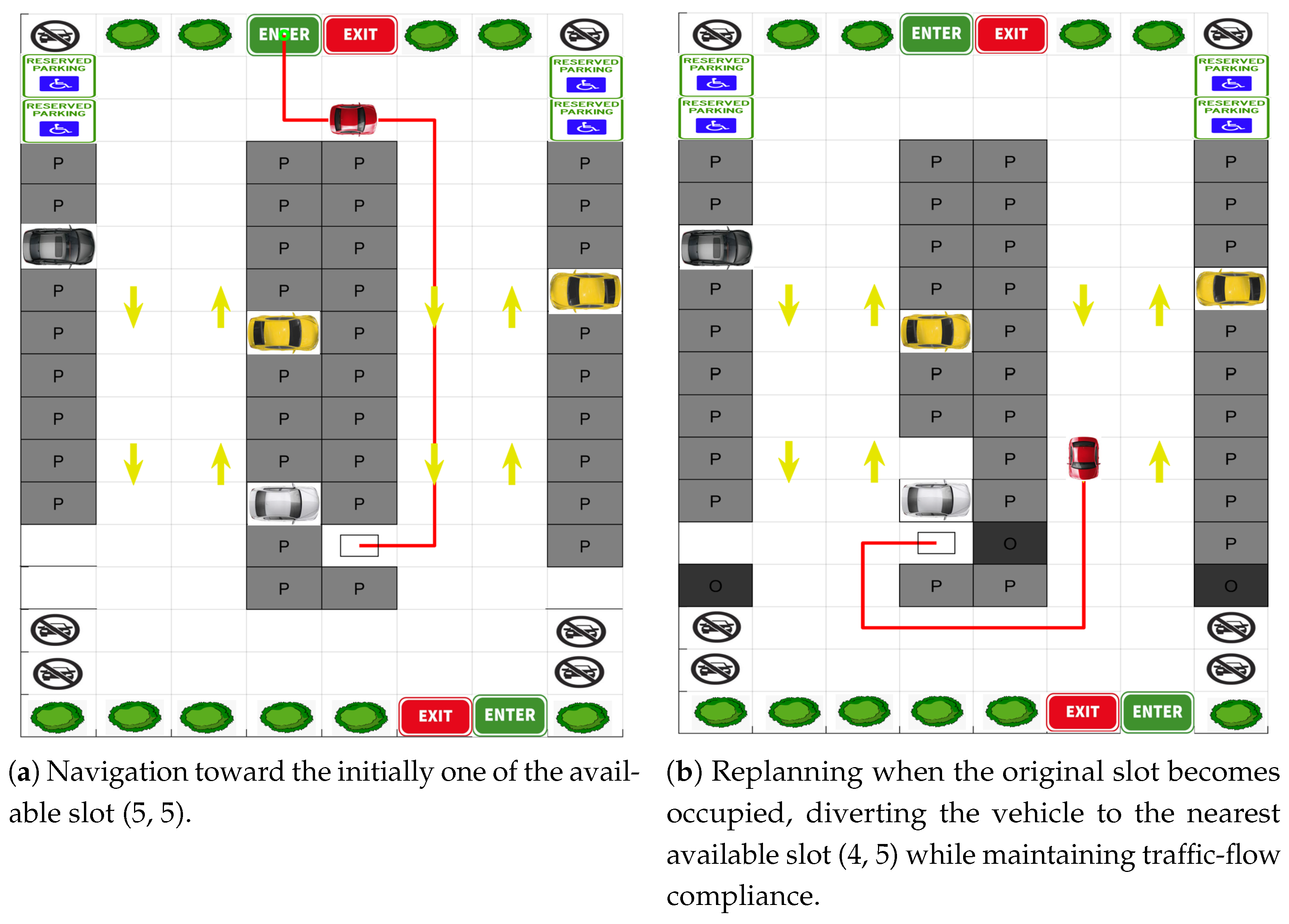
Experiment 4 (Figure 13a,b) explores the SPTL planner’s ability to handle real-time goal updates in a smart parking environment. The simulation takes place in a $17\times 8$ grid-based parking lot where one-way lanes and reserved parking zones are strictly enforced.

At the start (Figure 13a), the ego vehicle (red) enters through the designated gate and navigates toward the nearest available parking slot at coordinate $(5, 5)$. The route follows all traffic flow constraints while minimizing travel distance. However, as the vehicle approaches the target, the slot at $(5, 5)$ becomes suddenly occupied by another vehicle, represented by a black obstacle (O) in (Figure 13b). Simultaneously, new vacant slots appear at $(4, 5)$ and $(4, 7)$. Leveraging the SPTL framework’s dynamic replanning capability, the ego vehicle recomputes its trajectory to reach the nearest available slot $(4, 5)$ while continuing to obey the one-way directional constraints.

This experiment demonstrates the system’s ability to adapt instantly to environmental changes such as sudden slot occupancy or newly available spaces. The SPTL planner maintains lawful motion, traffic compliance, and a collision-free path while achieving an updated goal under temporal-logic task constraints.

The mean total computation time was $0.5061\pm 0.0116$ s. The mean initial PA generation time was $0.4107\pm 0.0074$ s. The planner computed the initial path segment before replanning in $0.0142\pm 0.0017$ s, and recomputed the trajectory after replanning in $0.0029\pm 0.0003$ s. The PA rebuild during replanning was completed in $0.0076\pm 0.0008$ s. All performance metrics exhibited low variance, underscoring the consistency and efficiency of the proposed approach. These results indicate that the framework introduces negligible computational burden during slot reassignment and preserves real-time responsiveness. The planner’s reliable performance under dynamically changing parking-slot availability confirms its suitability for deployment in smart parking systems requiring lawful motion, rapid adaptation, and collision-free goal reassignment under LTL constraints.

5.5. Experiment 5: Multi-Stage Task Execution with Dynamic Re-Planning

This final experiment evaluates the planner’s performance in a large-scale, complex logistics scenario within a $28\times 35$ grid environment. The ego vehicle is assigned a sequential, multi-stage mission involving both drop-off and pick-up operations.

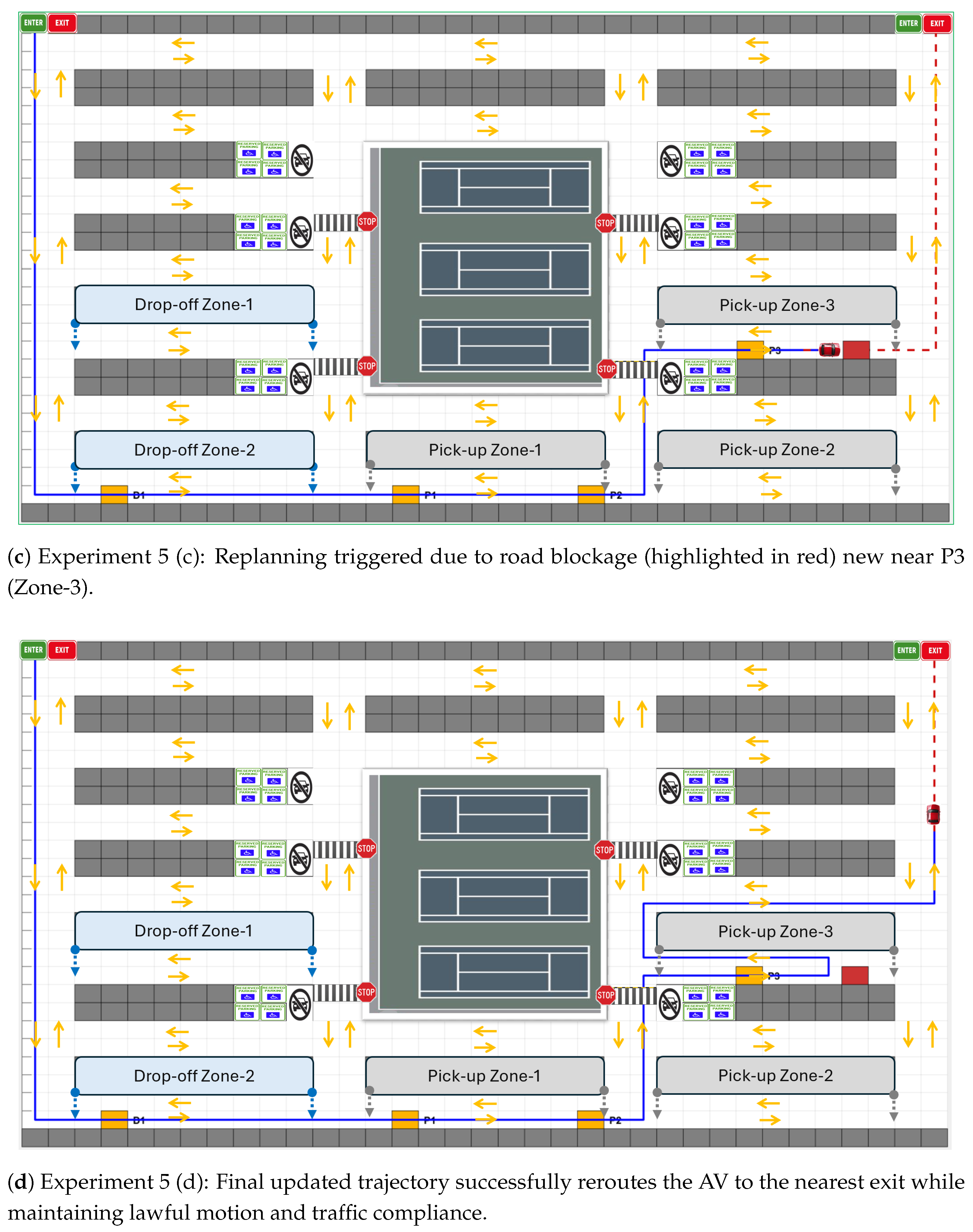
As illustrated in Figure 14a, the ego vehicle enters the facility and navigates to the first task, a drop-off at D1 $(4, 2)$. Upon completion, it proceeds to the first pick-up location, P1 $(15, 2)$, and then to the second, P2 $(22, 2)$. A dynamic task cancellation event is introduced in Figure 14b. While the ego vehicle is en route to the third pick-up, P3 $(32, 2)$, it receives a real-time update that this task has been canceled. The planner immediately invalidates the current path and re-evaluates the mission. It identifies the next pending task, originally designated P4 $(28, 10)$, re-assigns it as the new priority pick-up, and computes an optimal, traffic-compliant path to this new location. After servicing this task, the vehicle plans its route to the nearest exit. As shown in Figure 14c, it then encounters a sudden, long-term road blockage (visualized in red) at coordinate $(32, 10)$, rendering the initial exit path infeasible. In response, the system triggers a final replan. Figure 14d shows the new trajectory that successfully navigates the vehicle around the obstacle, adheres to all traffic-flow constraints, and directs it to the nearest available exit.

This scenario demonstrates the ego vehicle’s capability to execute complex, sequential logistics tasks in a large-scale environment while maintaining responsiveness to real-world uncertainties such as task cancellations and avoiding sudden obstacles. The test underscores the vehicle’s integration of logical task formulation, environmental awareness, and contributing to efficient and reliable operation in autonomous parking and mobility-on-demand systems.

The mean total computation time across 25 simulation runs was $4.1330\pm 0.1741$ s, with the initial PA generation time averaging $0.4266\pm 0.0084$ s. The planner computed the initial path segment in $0.0580\pm 0.0026$ s and, after each dynamic replanning event, recomputed updated trajectories in $0.0254\pm 0.0024$ s. The PA rebuilds triggered by runtime updates (e.g., task cancellations or obstacle appearances) were completed in $0.0284\pm 0.0024$ s. Although the total computation time increased due to the large-scale grid and multi-stage logistics complexity, all per-event replanning steps exhibited low standard deviation and tight latency bounds. These results confirm that the SPTL-based planner maintains consistent and deterministic responsiveness under dynamically evolving, real-world conditions—supporting reliable execution of complex mission sequences involving task cancellation, obstacle avoidance, and goal reassignment in structured parking environments.

5.6. Quantitative Comparison and Performance Trends

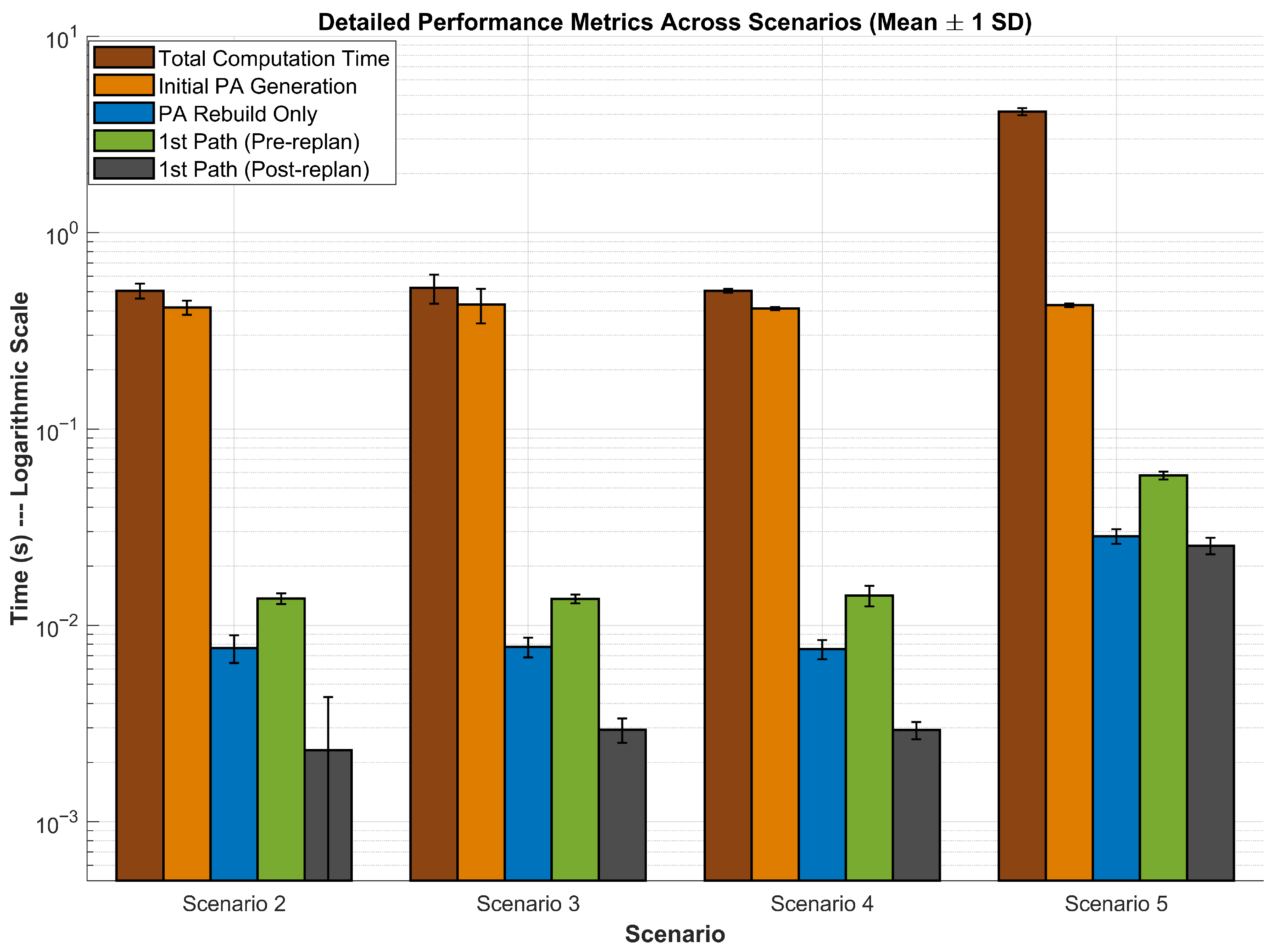
Figure 15 provides a detailed breakdown of five key computational components across four benchmark scenarios (Scenarios 2–5), with each bar depicting the mean value over 25 runs and corresponding standard deviation on a logarithmic Y-axis. This visualization highlights the scalability and efficiency of the SPTL planner across diverse operating conditions.

The total computation time (brown bars) captures the aggregate planning effort, inclusive of initial and replanning phases. Scenario 5 demonstrates the highest overall planning cost (∼4.13 s), driven by the compound complexity of dynamic replanning. In contrast, Scenarios 2 through 4 maintain significantly lower totals, around ∼0.51–0.52 s on average.

The initial PA generation time (orange bars) remains relatively stable across scenarios, averaging ∼0.41–0.43 s, and reflects the primary offline synthesis cost. The PA rebuild time during dynamic replanning (blue bars) is minimal in all cases (∼0.0076–0.028 s), showcasing the planner’s real-time adaptability under task or environment modifications.

Path computation times before and after replanning (green and black bars, respectively) further dissect planning responsiveness. Pre-replanning path synthesis consistently requires ∼0.013–0.058 s, while post-replanning path generation remains even faster (∼0.0023–0.025 s). Notably, both metrics show low variance, reinforcing temporal predictability.

A numerical summary of these timing metrics is presented in

Table 6. Summary of Quantitative Insights.

Scenario	Mean Total Computation Time (s)	Replanning Latency (s)
2	$0.5061\pm 0.0442$	$0.0023\pm 0.0020$ (post-replan),
		$0.0077\pm 0.0012$ (PA rebuild)
3	$0.5231\pm 0.0886$	$0.0029\pm 0.0004$ (post-replan),
		$0.0078\pm 0.0009$ (PA rebuild)
4	$0.5061\pm 0.0116$	$0.0029\pm 0.0003$ (post-replan),
		$0.0076\pm 0.0008$ (PA rebuild)
5	$4.1330\pm 0.1741$	$0.0254\pm 0.0024$ (post-replan),
		$0.0284\pm 0.0024$ (PA rebuild)

, which consolidates the mean and standard deviation values for total computation and key replanning latencies. The table substantiates the graphical trends with precise numerical evidence, further validating the framework’s consistent low-latency performance across heterogeneous planning conditions.

5.7. Experiment 6: Comparative Benchmark of Replanning Computation

To directly quantify the computational advantages of our proposed framework—a key contribution highlighted in the Abstract—this experiment provides a direct performance comparison between our matrix-based method and a traditional automata-theoretic approach. While Experiments 1–5 validate the planner’s correctness and agility in dynamic scenarios, this experiment is designed to isolate and measure the computational gain of its underlying construction, particularly in a dynamic replanning scenario where the LTL task itself changes.

We compare two methods for generating a Product Automaton for the $35\times 28$ environment:

• Our Proposed Matrix-Based Method: This method first computes the atomic proposition matrices (e.g., $M_b^{\mathcal{G}}$, $M_c^{\mathcal{G}}$) once. It then constructs the final Product Automaton matrix ($P{A}_{\mathrm{Auto}1}$) using Boolean operations. When a new task ($LT{L}_2$) is given, it reuses the atomic matrices and only re-runs the Boolean operations to build $P{A}_{\mathrm{Auto}2}$.
• Traditional Automata-Based Method: This method iterates through every environment state and task state to build the product automaton “from scratch” for $LT{L}_1$. When the task changes to $LT{L}_2$, it must discard its previous work and re-run the entire “from-scratch” iterative process.

We timed both methods for two distinct LTL tasks:

• Task 1: “$\mathsf{F}\mathrm{goal}\wedge (\neg \mathrm{goal}\mathsf{U}\mathrm{pick})$”
• Task 2: “$\mathsf{F}(\mathrm{pick}\wedge \mathsf{F}\mathrm{goal})$”

Table 7. Benchmark results comparing matrix-based vs. traditional automata-based Product Automaton computation.

Method	Task 1 (Initial Build)	Task 2 (Replanning)	Total Time
Our Matrix-Based Method	$0.4302\pm 0.0081$ s	$0.3952\pm 0.0019$ s	$0.8254\pm 0.0094$ s
Traditional Method	$0.8316\pm 0.0151$ s	$0.7935\pm 0.0123$ s	$2.4248\pm 0.0238$ s

summarizes the benchmark comparison between our matrix-based and the traditional automata-based product automaton computation methods across two tasks: initial build and replanning. The results yield three critical insights.

• Initial Computation Speed: Our matrix-based method demonstrates a significant performance advantage, completing the initial build in $0.4302$ s compared to $0.8316$ s for the traditional method. This represents a 1.93× speedup, attributable to the efficient vectorized matrix operations utilized in our framework.
• Replanning Efficiency (Key Contribution): For the replanning phase, our method completes Task 2 in $0.3952$ s, whereas the traditional method requires $0.7935$ s. This reflects a 2.01× speedup, highlighting the matrix-based method’s architectural efficiency for dynamic replanning. Notably, our approach avoids full reconstruction of the product automaton during replanning, in contrast to the traditional method which re-executes the entire computation pipeline. Optionally, this also explains why our Task 2 is faster than even our Task 1 (by ∼1.09×), due to the reuse of atomic propositions instead of recomputation.
• Total Computation Time: When combining both tasks, the matrix-based method completes planning in $0.8254$ s on average—over 2.94× faster than the traditional method’s $2.4248$ s. This underscores the method’s suitability for time-critical applications requiring both initial and reactive planning responsiveness.

This experiment confirms that our matrix-based construction is not only significantly faster for initial planning but is also architected for efficient, real-time replanning, directly addressing the scalability and dynamic adaptability challenges present in the state-of-the-art.

Collectively, Experiments 1–6 validate the robustness, agility, and real-world readiness of the SPTL-based planning architecture across diverse autonomous-driving scenarios. The framework demonstrated adaptability to task modifications, compliance with traffic-flow rules, and seamless goal-oriented replanning under varying constraints (Experiments 1–4). It effectively managed dynamic environmental changes such as occupied parking slots and unexpected obstacles, while scaling efficiently to multi-stage missions involving drop-offs, cancellations, and rerouting (Experiment 5). Quantitatively, total computation time scaled with scenario complexity, whereas replanning latency remained consistently low and stable.

Furthermore, Experiment 6 provided updated empirical evidence demonstrating that the proposed matrix-based construction is over 1.9× faster for initial product automaton computation compared to traditional methods (0.4302 s vs. 0.8316 s). More critically, our approach achieves approximately 2.0× faster performance in replanning (0.3952 s vs. 0.7935 s), highlighting its architectural advantage in reusing atomic propositions rather than reconstructing them from scratch. This reuse leads not only to significantly reduced computation time but also to improved responsiveness under dynamic conditions. Together, these results affirm that the proposed SPTL framework offers a unified, logically grounded, computationally efficient, and real-time capable solution for safe, rule-compliant, and adaptive navigation in parking environments.

6. Conclusions

This paper addressed the complex challenge of autonomous vehicle navigation in a parking environments under LTL constraints. The proposed matrix-based framework unified spatial connectivity and behavioral constraints into a single product automaton representation, enabling efficient path planning using Dijkstra’s algorithm. Through five progressively complex experiments, the results substantiated the framework’s robustness, adaptability, and computational efficiency.

The experiments demonstrated that the SPTL-based planner could dynamically adapt to environmental changes such as obstacles, one-way rule enforcement, slot occupancy, and cancellations while maintaining strict compliance with LTL constraints. Quantitatively, the planner sustained low and consistent replanning latencies (0.016–0.034 s), despite total computation times scaling with scenario complexity—from 0.04 s to 4.13 s. Additionally, a direct benchmark (Experiment 6) confirmed that the matrix-based method achieves over 2.1× faster initial product automaton generation and ∼2× faster replanning than traditional iterative methods, owing to atomic reuse. These findings validate the planner’s responsiveness, goal-oriented performance, and scalability under both static and dynamic planning contexts.

Future work will focus on extending this architecture to multi-vehicle unparking coordination for larger fleets. Additionally, the focus will include backing maneuvers during unparking, addressing critical safety concerns associated with pedestrian fatalities. Ultimately, this research underscores the viability of formal verification methods in enhancing the safety, reliability, and adaptability of autonomous navigation systems.

References

1. Miao, X.; Duan, M. A Study on Parking Problems and Countermeasures of Urban Central Commercial District. In Proceedings of the International Conference on Electrical and Information Technologies for Rail Transportation-Volume II; Springer: Berlin/Heidelberg, Germany, 2014; pp. 601–608. [Google Scholar]
2. Wang, D.; Liang, H.; Mei, T.; Zhu, H. Research on self-parking path planning algorithms. In Proceedings of the IEEE International Conference on Vehicular Electronics and Safety, Beijing, China, 10–12 July 2011; pp. 258–262. [Google Scholar] [CrossRef]
3. Cookson, G.; Pishue, B. The Impact of Parking Pain in the US, UK and Germany. Available online: https://www2.inrix.com/research-parking-2017 (accessed on 10 June 2024).
4. Shoup, D.C. Cruising for parking. Transp. Policy 2006, 13, 479–486. [Google Scholar] [CrossRef]
5. Transline. Parking Lot Accident Statistics–Making Parking Lots Safer. 2023. Available online: https://translineinc.com/parking-lot-accident-statistics/ (accessed on 11 June 2024).
6. National Highway Traffic Safety Administration. Traffic Safety Facts 2020: A Compilation of Motor Vehicle Crash Data; Technical Report; National Highway Traffic Safety Administration, U.S. Department of Transportation: Washington, DC, USA, 2020. [Google Scholar]
7. GITNUX. Parking Lot Accident Statistics [Fresh Research]. 2024. Available online: https://gitnux.org/parking-lot-accident-statistics/#content (accessed on 11 June 2024).
8. National Highway Traffic Safety Administration. Non-Traffic Surveillance (NTS). 2024. Available online: https://www.nhtsa.gov/crash-data-systems/non-traffic-surveillance (accessed on 12 June 2024).
9. National Safety Council. Pedestrians: Data Details. 2024. Available online: https://injuryfacts.nsc.org/motor-vehicle/road-users/pedestrians/data-details/ (accessed on 12 June 2024).
10. Nations, U. 68% of the World Population Projected to Live in Urban Areas by 2050, Says UN. 2023. Available online: https://www.un.org/development/desa/en/news/population/2018-revision-of-world-urbanization-prospects.html (accessed on 11 June 2024).
11. Rupareliya, P.K. IOT in Smart Parking System—Problems, Solutions, Applications. 2022. Available online: https://www.intuz.com/blog/iot-in-smart-parking-management-benefits-challenges (accessed on 11 June 2024).
12. Mulloy, R. Solving Parking Challenges with Smart Solutions and Innovations. 2023. Available online: https://operationscommander.com/blog/parking-management-challenges/ (accessed on 11 June 2024).
13. Daxwanger, W.; Schmidt, G. Skill-based visual parking control using neural and fuzzy networks. In Proceedings of the IEEE International Conference on Systems, Man and Cybernetics. Intelligent Systems for the 21st Century, Vancouver, BC, Canada, 22–25 October 1995; Volume 2, pp. 1659–1664. [Google Scholar] [CrossRef]
14. Gorinevsky, D.; Kapitanovsky, A.; Goldenberg, A. Neural network architecture for trajectory generation and control of automated car parking. IEEE Trans. Control Syst. Technol. 1996, 4, 50–56. [Google Scholar] [CrossRef]
15. Nguyen, D.; Widrow, B. Neural networks for self-learning control systems. IEEE Control Syst. Mag. 1990, 10, 18–23. [Google Scholar] [CrossRef]
16. Shirazi, B.; Yih, S. Learning to control: A heterogeneous approach. In Proceedings of the IEEE International Symposium on Intelligent Control, Albany, NY, USA, 25–26 September 1989; pp. 320–325. [Google Scholar] [CrossRef]
17. Sugeno, M.; Murakami, K. Fuzzy parking control of model car. In Proceedings of the 23rd IEEE Conference on Decision and Control, Las Vegas, NV, USA, 12–14 December 1984; pp. 902–903. [Google Scholar]
18. Li, T.H.S.; Chang, S.J.; Chen, Y.X. Implementation of human-like driving skills by autonomous fuzzy behavior control on an FPGA-based car-like mobile robot. IEEE Trans. Ind. Electron. 2003, 50, 867–880. [Google Scholar] [CrossRef]
19. Li, T.H.S.; Chang, S.J. Autonomous Fuzzy Parking Control of a Car-Like Mobile Robot. IEEE Trans. Syst. Man Cybern. Part A Syst. Hum. 2003, 33, 451–465. [Google Scholar] [CrossRef]
20. Leitch, D.; Probert, P. New techniques for genetic development of a class of fuzzy controllers. IEEE Trans. Syst. Man Cybern. Part C Appl. Rev. 1998, 28, 112–123. [Google Scholar] [CrossRef]
21. Zhao, Y.; Collins, E.G. Robust automatic parallel parking in tight spaces via fuzzy logic. Robot. Auton. Syst. 2005, 51, 111–127. [Google Scholar] [CrossRef]
22. Lee, J.Y.; Lee, J.J. Multiple Designs of Fuzzy Controllers for Car Parking Using Evolutionary Algorithm. In Proceedings of the IEEE International Conference on Mechatronics, Harbin, China, 5–9 May 2007; pp. 1–6. [Google Scholar]
23. Ryu, Y.W.; Oh, S.Y.; Kim, S. Robust Automatic Parking without Odometry Using Enhanced Fuzzy Logic Controller. In Proceedings of the IEEE International Conference on Fuzzy Systems, Vancouver, BC, Canada, 16–21 July 2006; pp. 521–527. [Google Scholar] [CrossRef]
24. Dolgov, D.; Thrun, S.; Montemerlo, M.; Diebel, J. Practical Search Techniques in Path Planning for Autonomous Driving. In Proceedings of the Eighteenth International Conference on Automated Planning and Scheduling, Sydney, Australia, 14–18 September 2008. [Google Scholar]
25. Montemerlo, M.; Becker, J.; Bhat, S.; Dahlkamp, H.; Dolgov, D.; Ettinger, S.; Haehnel, D.; Hilden, T.; Hoffmann, G.; Huhnke, B.; et al. Junior: The Stanford Entry in the Urban Challenge. J. Field Robot. 2008, 25, 569–597. [Google Scholar] [CrossRef]
26. Qin, Z.; Chen, X.; Hu, M.; Chen, L.; Fan, J. A novel path planning methodology for automated valet parking based on directional graph search and geometry curve. Robot. Auton. Syst. 2020, 132, 103606. [Google Scholar] [CrossRef]
27. Sedighi, S.; Nguyen, D.V.; Kapsalas, P.; Kuhnert, K.D. Implementing Voronoi-based Guided Hybrid A* in Global Path Planning for Autonomous Vehicles. In Proceedings of the IEEE Intelligent Transportation Systems Conference, Auckland, New Zealand, 27–30 October 2019; pp. 3845–3852. [Google Scholar]
28. Sheng, W.; Li, B.; Zhong, X. Autonomous Parking Trajectory Planning With Tiny Passages: A Combination of Multistage Hybrid A-Star Algorithm and Numerical Optimal Control. IEEE Access 2021, 9, 102801–102810. [Google Scholar] [CrossRef]
29. Pang, J.; Zhang, S.; Fu, J.; Liu, J.; Zheng, N. Curvature Continuous Path Planning with Reverse Searching for Efficient and Precise Autonomous Parking. In Proceedings of the IEEE 25th International Conference on Intelligent Transportation Systems, Macau, China, 8–12 October 2022; pp. 2798–2805. [Google Scholar] [CrossRef]
30. Zhang, X.; Liniger, A.; Sakai, A.; Borrelli, F. Autonomous Parking Using Optimization-Based Collision Avoidance. In Proceedings of the IEEE Conference on Decision and Control, Miami Beach, FL, USA, 17–19 December 2018; pp. 4327–4332. [Google Scholar] [CrossRef]
31. Wu, Y.; Li, X.; Gao, J.; Yang, X. Research on Automatic Vertical Parking Path-Planning Algorithms for Narrow Parking Spaces. Electronics 2023, 12, 4203. [Google Scholar] [CrossRef]
32. Esposto, F.; Goos, J.; Teerhuis, A.; Alirezaei, M. Hybrid path planning for non-holonomic autonomous vehicles: An experimental evaluation. In Proceedings of the 5th IEEE International Conference on Models and Technologies for Intelligent Transportation Systems, Naples, Italy, 26–28 June 2017; pp. 25–30. [Google Scholar]
33. Conner, D.C.; Kress-Gazit, H.; Choset, H.; Rizzi, A.A.; Pappas, G.J. Valet parking without a valet. In Proceedings of the IEEE/RSJ International Conference on Intelligent Robots and Systems, San Diego, CA, USA, 29 October–2 November 2007; pp. 572–577. [Google Scholar] [CrossRef]
34. Antoniotti, M.; Mishra, B. Discrete event models+temporal logic=supervisory controller: Automatic synthesis of locomotion controllers. In Proceedings of the IEEE International Conference on Robotics and Automation, Nagoya, Japan, 21–27 May 1995; Volume 2, pp. 1441–1446. [Google Scholar] [CrossRef]
35. Fainekos, G.; Kress-Gazit, H.; Pappas, G. Temporal Logic Motion Planning for Mobile Robots. In Proceedings of the IEEE International Conference on Robotics and Automation, Barcelona, Spain, 18–22 April 2005; pp. 2020–2025. [Google Scholar] [CrossRef]
36. Belta, C.; Isler, V.; Pappas, G. Discrete abstractions for robot motion planning and control in polygonal environments. IEEE Trans. Robot. 2005, 21, 864–874. [Google Scholar] [CrossRef]
37. Wongpiromsarn, T.; Topcu, U.; Murray, R.M. Receding horizon temporal logic planning for dynamical systems. In Proceedings of the 48h IEEE Conference on Decision and Control Held Jointly with 28th Chinese Control Conference, Shanghai, China, 16–18 December 2009; pp. 5997–6004. [Google Scholar] [CrossRef]
38. Jiang, F.J.; Gao, Y.; Xie, L.; Johansson, K.H. Ensuring safety for vehicle parking tasks using Hamilton-Jacobi reachability analysis. In Proceedings of the 59th IEEE Conference on Decision and Control, Jeju Island, Republic of Korea, 14–18 December 2020; pp. 1416–1421. [Google Scholar] [CrossRef]
39. Badithela, A.; Graebener, J.; Murray, R.M. Minimally Constrained Testing for Autonomy with Temporal Logic Specifications. In Proceedings of the RSS Workshop on Envisioning an Infrastructure for Multi-Robot and Collaborative Autonomy Testing and Evaluation, New York, NY, USA, 26–27 June 2022; Robotics: Science and Systems Foundation: New York, NY, USA, 2022. [Google Scholar]
40. Lee, S.H.; Seo, S.W. A Learning-Based Framework for Handling Dilemmas in Urban Automated Driving. In Proceedings of the IEEE International Conference on Robotics and Automation, Singapore, 29 May–3 June 2017; pp. 1436–1442. [Google Scholar]
41. Abbeel, P.; Dolgov, D.; Ng, A.Y.; Thrun, S. Apprenticeship Learning for Motion Planning with Application to Parking Lot Navigation. In Proceedings of the IEEE/RSJ International Conference on Intelligent Robots and Systems, Nice, France, 22–26 September 2008; pp. 1083–1090. [Google Scholar]
42. Aatif, M.; Baig, M.Z.; Adeel, U.; Rashid, A. Path Planning with Adaptive Autonomy Based on an Improved A* Algorithm and Dynamic Programming for Mobile Robots. Information 2025, 16, 700. [Google Scholar] [CrossRef]
43. Lee, C.K.; Lin, C.L.; Shiu, B.M. Autonomous Vehicle Parking Using Hybrid Artificial Intelligent Approach. J. Intell. Robot. Syst. 2009, 56, 319–343. [Google Scholar] [CrossRef]
44. Nakrani, N.; Joshi, M. An Intelligent Fuzzy based Hybrid Approach for Parallel Parking in Dynamic Environment. Procedia Comput. Sci. 2018, 133, 82–91. [Google Scholar] [CrossRef]
45. Kong, S.G.; Kosko, B. Comparison of fuzzy and neural truck backer-upper control systems. In Proceedings of the International Joint Conference on Neural Networks, San Diego, CA, USA, 17–21 June 1990; Volume 3, pp. 349–358. [Google Scholar] [CrossRef]
46. Yasunobu, S.; Murai, Y. Parking control based on predictive fuzzy control. In Proceedings of the IEEE 3rd International Fuzzy Systems Conference, Orlando, FL, USA, 26–29 June 1994; Volume 2, pp. 1338–1341. [Google Scholar] [CrossRef]
47. Leu, M.; Kim, T.Q. Cell mapping based fuzzy control of car parking. In Proceedings of the IEEE International Conference on Robotics and Automation (Cat. No.98CH36146), Leuven, Belgium, 20 May 1998; Volume 3, pp. 2494–2499. [Google Scholar] [CrossRef]
48. Gómez-Bravo, F.; Cuesta, F.; Ollero, A. Parallel and diagonal parking in nonholonomic autonomous vehicles. Eng. Appl. Artif. Intell. 2001, 14, 419–434. [Google Scholar] [CrossRef]
49. Li, T.H.S.; Yeh, Y.C.; Wu, J.D.; Hsiao, M.Y.; Chen, C.Y. Multifunctional Intelligent Autonomous Parking Controllers for Carlike Mobile Robots. IEEE Trans. Ind. Electron. 2010, 57, 1687–1700. [Google Scholar] [CrossRef]
50. Meng, T.; Yang, T.; Huang, J.; Jin, W.; Zhang, W.; Jia, Y.; Wan, K.; Xiao, G.; Yang, D.; Zhong, Z. Improved Hybrid A-star Algorithm for Path Planning in Autonomous Parking System Based on Multi-Stage Dynamic Optimization. Int. J. Automot. Technol. 2023, 24, 459–468. [Google Scholar] [CrossRef]
51. Smith, S.L.; Tumova, J.; Belta, C.; Rus, D. Optimal path planning under temporal logic constraints. In Proceedings of the IEEE/RSJ International Conference on Intelligent Robots and Systems, Taipei, Taiwan, 18–22 October 2010; pp. 3288–3293. [Google Scholar] [CrossRef]
52. Sedighi, S.; Nguyen, D.V.; Kuhnert, K.D. Guided Hybrid A-star Path Planning Algorithm for Valet Parking Applications. In Proceedings of the 5th International Conference on Control, Automation and Robotics, Beijing, China, 19–22 April 2019; pp. 570–575. [Google Scholar] [CrossRef]
53. Shi, Y.; Wang, P.; Wang, X. An Autonomous Valet Parking Algorithm for Path Planning and Tracking. In Proceedings of the IEEE 96th Vehicular Technology Conference, London, UK, 26–29 September 2022; pp. 1–6. [Google Scholar] [CrossRef]
54. Zhang, Z.; Wan, Y.; Wang, Y.; Guan, X.; Ren, W.; Li, G. Improved Hybrid A* Path Planning Method for Spherical Mobile Robot Based on Pendulum. Int. J. Adv. Robot. Syst. 2021, 18, 1–14. [Google Scholar] [CrossRef]
55. Aatif, M.; Adeel, U.; Basiri, A.; Mariani, V.; Iannelli, L.; Glielmo, L. Deep Learning Based Path-Planning Using CRNN and A* for Mobile Robots. In Proceedings of the Second International Conference on Innovations in Computing Research; Daimi, K., Al Sadoon, A., Eds.; Springer Nature Switzerland: Cham, Switzerland, 2023; pp. 118–128. [Google Scholar]
56. Gao, Y.; Jiang, F.J.; Ren, X.; Xie, L.; Johansson, K.H. Reachability-based Human-in-the-Loop Control with Uncertain Specifications. IFAC-PapersOnLine 2020, 53, 1880–1887. [Google Scholar] [CrossRef]
57. Zhou, Y.; Maity, D.; Baras, J.S. Optimal mission planner with timed temporal logic constraints. In Proceedings of the European Control Conference, Linz, Austria, 15–17 July 2015; pp. 759–764. [Google Scholar]
58. Zhou, Y.; Maity, D.; Baras, J.S. Timed automata approach for motion planning using metric interval temporal logic. In Proceedings of the European Control Conference, Aalborg, Denmark, 29 June–1 July 2016; pp. 690–695. [Google Scholar]
59. Maity, D.; Baras, J.S. Event-triggered controller synthesis for dynamical systems with temporal logic constraints. In Proceedings of the American Control Conference, Milwaukee, WI, USA, 27–29 June 2018; pp. 1184–1189. [Google Scholar] [CrossRef]
60. Lindemann, L.; Maity, D.; Baras, J.S.; Dimarogonas, D.V. Event-triggered feedback control for signal temporal logic tasks. In Proceedings of the Conference on Decision and Control, Miami Beach, FL, USA, 17–19 December 2018; pp. 146–151. [Google Scholar]
61. Dolgov, D.; Thrun, S.; Montemerlo, M.; Diebel, J. Path planning for autonomous vehicles in unknown semi-structured environments. Int. J. Robot. Res. 2010, 29, 485–501. [Google Scholar] [CrossRef]
62. Shen, X.; Zhang, X.; Borrelli, F. Autonomous Parking of Vehicle Fleet in Tight Environments. In Proceedings of the American Control Conference, Denver, CO, USA, 1–3 July 2020; pp. 3035–3040. [Google Scholar] [CrossRef]
63. Du, X.; Tan, K.K. Autonomous Reverse Parking System Based on Robust Path Generation and Improved Sliding Mode Control. IEEE Trans. Intell. Transp. Syst. 2015, 16, 1225–1237. [Google Scholar] [CrossRef]
64. Muller, B.; Deutscher, J.; Grodde, S. Trajectory generation and feedforward control for parking a car. In Proceedings of the IEEE Conference on Computer Aided Control System Design, IEEE International Conference on Control Applications, IEEE International Symposium on Intelligent Control, Andras Varga, PC, USA, 4–6 October 2006; pp. 163–168. [Google Scholar] [CrossRef]
65. Chen, C.; Wu, B.; Xuan, L.; Chen, J.; Wang, T.; Qian, L. A trajectory planning method for autonomous valet parking via solving an optimal control problem. Sensors 2020, 20, 6435. [Google Scholar] [CrossRef]
66. Li, B.; Shao, Z. A Unified Motion Planning Method for Parking an Autonomous Vehicle in the Presence of Irregularly Placed Obstacles. Knowl.-Based Syst. 2015, 86, 11–20. [Google Scholar] [CrossRef]
67. Ohata, A.; Mio, M. Parking Control Based on Nonlinear Trajectory Control for Low Speed Vehicles. In Proceedings of the International Conference on Industrial Electronics, Control and Instrumentation, Kobe, Japan, 28 October–1 November 1991; pp. 107–112. [Google Scholar]
68. Müller, B.; Deutscher, J.; Grodde, S. Continuous Curvature Trajectory Design and Feedforward Control for Parking a Car. IEEE Trans. Control Syst. Technol. 2007, 15, 541–552. [Google Scholar] [CrossRef]
69. Gómez-Bravo, F.; Cuesta, F.; Ollero, A.; Viguria, A. Continuous Curvature Path Generation Based on β-Spline Curves for Parking Manoeuvres. Robot. Auton. Syst. 2008, 56, 360–372. [Google Scholar] [CrossRef]
70. Vorobieva, H.; Minoiu-Enache, N.; Glaser, S.; Mammar, S. Geometric Continuous-Curvature Path Planning for Automatic Parallel Parking. In Proceedings of the 10th IEEE International Conference on Networking, Sensing and Control, Evry, France, 10–12 April 2013; pp. 418–423. [Google Scholar] [CrossRef]
71. Yang, W. Optimal Approach for Autonomous Parallel Parking of Nonholonomic Car-Like Vehicle. Master’s Thesis, State University of New York at Buffalo, Department of Mechanical & Aerospace Engineering, Buffalo, NY, USA, 2006. [Google Scholar]
72. Patten, W.N.; Wu, H.C.; Cai, W. Perfect Parallel Parking Via Pontryagin’s Principle. J. Dyn. Syst. Meas. Control 1994, 116, 723–728. [Google Scholar] [CrossRef]
73. Kondak, K.; Hommel, G. Computation of Time Optimal Movements for Autonomous Parking of Non-Holonomic Mobile Platforms. In Proceedings of the IEEE International Conference on Robotics and Automation, Seoul, Republic of Korea, 21–26 May 2001; pp. 2698–2703. [Google Scholar]
74. Li, B.; Wang, K.; Shao, Z. Time-Optimal Maneuver Planning in Automatic Parallel Parking Using a Simultaneous Dynamic Optimization Approach. IEEE Trans. Intell. Transp. Syst. 2016, 17, 3263–3274. [Google Scholar] [CrossRef]
75. Vorobieva, H.; Glaser, S.; Minoiu-Enache, N.; Mammar, S. Automatic Parallel Parking in Tiny Spots: Path Planning and Control. IEEE Trans. Intell. Transp. Syst. 2015, 16, 396–409. [Google Scholar] [CrossRef]
76. Wang, J.; Li, J.; Yang, J.; Meng, X.; Fu, T. Automatic Parking Trajectory Planning Based on Random Sampling and Nonlinear Optimization. J. Frankl. Inst. 2023, 360, 9579–9601. [Google Scholar] [CrossRef]
77. Zips, P.; Böck, M.; Kugi, A. Optimisation Based Path Planning for Car Parking in Narrow Environments. Robot. Auton. Syst. 2016, 79, 1–11. [Google Scholar] [CrossRef]
78. Zips, P.; Böck, M.; Kugi, A. Fast Optimization Based Motion Planning and Path-Tracking Control for Car Parking. In Proceedings of the 9th IFAC Symposium on Nonlinear Control Systems, Toulouse, France, 4–6 September 2013; pp. 86–91. [Google Scholar] [CrossRef]
79. Zhu, M.; Liu, Q.; Zhou, J.; Sha, W.; Niu, R. Autonomous Parking Path Tracking Control Based on Interference Suppression. IEEE Access 2023, 11, 109528–109538. [Google Scholar] [CrossRef]
80. Chen, L.; Qin, Z.; Hu, M.; Bian, Y.; Peng, X. Path Tracking Controller Design of Automated Parking Systems via NMPC with an Instructible Solution. Chin. J. Mech. Eng. 2024, 37, 65. [Google Scholar] [CrossRef]
81. Ferguson, D.; Howard, T.M.; Likhachev, M. Motion Planning in Urban Environments: Part I. In Proceedings of the IEEE/RSJ International Conference on Intelligent Robots and Systems, Nice, France, 22–26 September 2008; pp. 1063–1069. [Google Scholar]
82. Ferguson, D.; Howard, T.M.; Likhachev, M. Motion Planning in Urban Environments: Part II. In Proceedings of the IEEE/RSJ International Conference on Intelligent Robots and Systems, Nice, France, 22–26 September 2008; pp. 1070–1076. [Google Scholar]
83. Qin, Y.; Liu, F.; Wang, P. A Feasible Parking Algorithm in Form of Path Planning and Following. In Proceedings of the 3rd International Conference on Robotics and Artificial Intelligence, (RICAI), Shanghai, China, 20–22 September 2019; pp. 6–11. [Google Scholar] [CrossRef]
84. Richter, S.R.; Vineet, V.; Roth, S.; Koltun, V. Playing for Data: Ground Truth from Computer Games. arXiv 2016, arXiv:cs.CV/1608.02192. [Google Scholar] [CrossRef]
85. Phadnis, M. Latest Review of Parking Problems and Intelligent Parking System for Smart City. Int. J. Sci. Eng. Res. 2016, 7, 1275–1279. [Google Scholar]
86. Mazda USA. 2018 Mazda6 Owner’s Manual. Available online: https://www.mazdausa.com/static/manuals/2018/mazda6/contents/05200100.html. (accessed on 12 June 2024).
87. Diehl, C.; Makarow, A.; Rösmann, C.; Bertram, T. Time-Optimal Nonlinear Model Predictive Control for Radar-based Automated Parking. IFAC-PapersOnLine 2022, 55, 34–39. [Google Scholar] [CrossRef]
88. Su-Jin, P.; Lebeltel, O.; Laugier, C. Parking a car using Bayesian Programming. In Proceedings of the 7th International Conference on Control, Automation, Robotics and Vision, Singapore, 2–5 December 2002; Volume 2, pp. 728–733. [Google Scholar] [CrossRef]
89. Dai, S.; Wang, Y. Long-Horizon Motion Planning for Autonomous Vehicle Parking Incorporating Incomplete Map Information. In Proceedings of the IEEE International Conference on Robotics and Automation, Xi’an, China, 30 May–5 June 2021; pp. 8135–8142. [Google Scholar] [CrossRef]
90. Kalašová, A.; Čulík, K.; Poliak, M.; Otahálová, Z. Smart Parking Applications and Its Efficiency. Sustainability 2021, 13, 6031. [Google Scholar] [CrossRef]
91. Hsieh, M.F.; Özguner, Ü. A Parking Algorithm for an Autonomous Vehicle. In Proceedings of the IEEE Intelligent Vehicles Symposium, Eindhoven, The Netherlands, 4–6 June 2008; pp. 1155–1160. [Google Scholar]
92. Paromtchik, I.E.; Laugier, C. Motion Generation and Control for Parking an Autonomous Vehicle. In Proceedings of the IEEE International Conference on Robotics and Automation, Minneapolis, MI, USA, 22–28 April 1996; pp. 3117–3122. [Google Scholar]
93. Paromtchik, I.E.; Laugier, C. Automatic Parallel Parking and Returning to Traffic Maneuvers. In Proceedings of the IEEE/RSJ International Conference on Intelligent Robots and Systems, Grenoble, France, 11 September 1997; pp. 3117–3122. [Google Scholar]
94. Sedighi, S.; Nguyen, D.V.; Kuhnert, K.D. Implementation of a Parking State Machine on Vision-Based Auto Parking Systems for Perpendicular Parking Scenarios. In Proceedings of the 6th International Conference on Control, Decision and Information Technologies, Paris, France, 23–26 April 2019; pp. 1711–1716. [Google Scholar]
95. Kümmerle, R.; Hähnel, D.; Dolgov, D.; Thrun, S.; Burgard, W. Autonomous Driving in a Multi-Level Parking Structure. In Proceedings of the IEEE International Conference on Robotics and Automation, Kobe, Japan, 12–17 May 2009; pp. 3395–3400. [Google Scholar]
96. Ahad, D.M.A.; Sarkar, A.A.; Mannan, M.A. Mathematical Modeling and to carry out a prototype helpmate differential drive robot for hospital purpose. Am. Acad. Sch. Res. J. 2014, 6, 1–15. [Google Scholar]
97. Grimmett, H.; Buerki, M.; Paz, L.; Pinies, P.; Furgale, P.; Posner, I.; Newman, P. Integrating Metric and Semantic Maps for Vision-Only Automated Parking. In Proceedings of the IEEE International Conference on Robotics and Automation, Seattle, WA, USA, 26–30 May 2015; pp. 2159–2166. [Google Scholar]
98. Schiotka, A.; Suger, B.; Burgard, W. Robot Localization with Sparse Scan-Based Maps. In Proceedings of the IEEE/RSJ International Conference on Intelligent Robots and Systems, Seattle, WA, USA, 26–30 September 2017; pp. 642–647. [Google Scholar]
99. Han, L.; Do, Q.H.; Mita, S. Unified Path Planner for Parking an Autonomous Vehicle based on RRT. In Proceedings of the IEEE International Conference on Robotics and Automation, Shanghai, China, 9–13 May 2011; pp. 5622–5627. [Google Scholar]
100. Kwon, H.; Chung, W. Performance Analysis of Path Planners for Car-Like Vehicles Toward Automatic Parking Control. Intell. Serv. Robot. 2014, 7, 15–23. [Google Scholar] [CrossRef]
101. Do, Q.H.; Mita, S.; Yoneda, K. A Practical and Optimal Path Planning for Autonomous Parking Using Fast Marching Algorithm and Support Vector Machine. IEICE Trans. Inf. Syst. 2013, E96-D, 2795–2804. [Google Scholar] [CrossRef]
102. Cai, L.; Guan, H.; Zhang, H.L.; Jia, X.; Zhan, J. Multi-maneuver Vertical Parking Path Planning and Control in a Narrow Space. Robot. Auton. Syst. 2022, 149, 103964. [Google Scholar] [CrossRef]
103. Vorobieva, H.; Glaser, S.; Minoiu-Enache, N.; Mammar, S. Automatic Parallel Parking with Geometric Continuous-Curvature Path Planning. In Proceedings of the IEEE Intelligent Vehicles Symposium (IV), Dearborn, MI, USA, 8–11 June 2014; pp. 465–471. [Google Scholar]
104. Vorobieva, H.; Glaser, S.; Minoiu-Enache, N.; Mammar, S. Geometric Path Planning for Automatic Parallel Parking in Tiny Spots. In Proceedings of the 13th IFAC Symposium on Control in Transportation Systems, Sofia, Bulgaria, 12–14 September 2012; pp. 36–42. [Google Scholar] [CrossRef]
105. Zheng, K.; Liu, S. RRT based Path Planning for Autonomous Parking of Vehicle. In Proceedings of the IEEE 7th Data Driven Control and Learning Systems Conference, Enshi, China, 25–27 May 2018; pp. 627–632. [Google Scholar]
106. Kuwata, Y.; Fiore, G.A.; Teo, J.; Frazzoli, E.; How, J.P. Motion Planning for Urban Driving using RRT. In Proceedings of the IEEE/RSJ International Conference on Intelligent Robots and Systems, Nice, France, 22–26 September 2008; pp. 1681–1686. [Google Scholar]
107. Jhang, J.H.; Lian, F.L.; Hao, Y.H. Human-like motion planning for autonomous parking based on revised bidirectional rapidly-exploring random tree* with Reeds-Shepp curve. Asian J. Control 2021, 23, 1146–1160. [Google Scholar] [CrossRef]
108. Dolgov, D.; Thrun, S. Autonomous Driving in Semi-Structured Environments: Mapping and Planning. In Proceedings of the IEEE International Conference on Robotics and Automation, Kobe, Japan, 12–17 May 2009; pp. 3407–3414. [Google Scholar]
109. AbuJabal, N.; Baziyad, M.; Fareh, R.; Brahmi, B.; Rabie, T.; Bettayeb, M. A Comprehensive Study of Recent Path-Planning Techniques in Dynamic Environments for Autonomous Robots. Sensors 2024, 24, 8089. [Google Scholar] [CrossRef]
110. Fersman, E.; Krcal, P.; Pettersson, P.; Yi, W. Task Automata: Schedulability, Decidability and Undecidability. Inf. Comput. 2007, 205, 1149–1172. [Google Scholar] [CrossRef]
111. Maity, D.; Baras, J.S. Motion Planning in Dynamic Environments with Bounded Time Temporal Logic Specifications. In Proceedings of the 2015 Mediterranean Conference on Control and Automation, Torremolinos, Spain, 16–19 June 2015; pp. 940–946. [Google Scholar]
112. Baier, C.; Katoen, J.P. Principles of Model Checking; MIT Press: Cambridge, MA, USA, 2008. [Google Scholar]
113. Kwiatkowska, M.; Norman, G.; Parker, D. PRISM 4.0—Verification of Probabilistic Real-Time Systems. In Computer Aided Verification, Lecture Notes in Computer Science; Springer: Berlin/Heidelberg, Germany, 2011; Volume 6806, pp. 585–591. [Google Scholar] [CrossRef]
114. Holzmann, G.J. The Model Checker SPIN. IEEE Trans. Softw. Eng. 1997, 23, 279–295. [Google Scholar] [CrossRef]
115. Duret-Lutz, A.; Lewkowicz, A.; Fauchille, A.; Michaud, T.; Renault, E.; Xu, L. Spot 2.0—A Framework for LTL and ω-automata Manipulation. In Automated Technology for Verification and Analysis, Lecture Notes in Computer Science; Springer: Berlin/Heidelberg, Germany, 2016; Volume 9938, pp. 122–129. [Google Scholar] [CrossRef]
116. Larsen, K.G.; Pettersson, P.; Yi, W. UPPAAL in a Nutshell. Int. J. Softw. Tools Technol. Transf. 1997, 1, 134–152. [Google Scholar] [CrossRef]
Figure 1. Convergence of Social and Technical Demands in Autonomous Parking.
Robotics 14 00171 g001
Figure 2. Automaton representation of a 6 × 4 parking grid. Blocked cells are shown in gray, v 0 is the start state (green), and the accepting state is highlighted in blue. Arrows are labeled with possible transitions (l: left, r: right, u: up, d: down).
Robotics 14 00171 g002
Figure 3. Sample parking scenario.
Robotics 14 00171 g003
Figure 4. System flow diagram for an algorithm. Node colors differentiate system components: blue for user inputs, green for algorithmic processes, and red for the conditional decision point.
Robotics 14 00171 g004
Figure 5. Environment automaton with all states a, c, d, and b marked as accepting (end) states. The left panel illustrates a 2 × 2 environment layout where location d is designated with a disability symbol to indicate accessibility. The right panel shows the corresponding environment automaton with transitions labeled by directional inputs: up (u), down (d), left (), and right (r). In this figure, the transition with ’1’ input correspond to a ‘stay’ action.
Robotics 14 00171 g005
Figure 6. Task automaton representing a sequence of region-based objectives. Here, φ is the LTL specification and ϕ is the sub-formulas that are on the transition of the task automaton.
Robotics 14 00171 g006
Figure 7. Product automaton.
Robotics 14 00171 g007
Figure 8. Pruned product automaton corresponding to the automaton in Figure 7.
Robotics 14 00171 g008
Figure 9. Experiment 1: Routing results for an autonomous vehicle. (a) Direct navigation to the exit, (b) Navigation with an intermediate pickup task, (c) Obstacle-induced re-planning.
Robotics 14 00171 g009
Figure 10. Dynamic obstacle handling using the SPTL-based planning algorithm.
Robotics 14 00171 g010
Figure 11. Realistic scenario validation using Driving Scenario Designer. Available at: https://www.youtube.com/watch?v=gDEEOHM1wgU (accessed on 12 November 2025).
Robotics 14 00171 g011
Figure 12. Agility test demonstrating dynamic goal adjustment and replanning.
Robotics 14 00171 g012
Figure 13. Dynamic parking-slot reassignment using the SPTL-based planner.
Robotics 14 00171 g013
Figure 14. Experiment 5 (a,b): Sequential mission execution and dynamic task cancellation in a 28 × 35 grid-based parking environment. (a) illustrates initial planning involving drop-off and multiple pick-up operations. (b) shows replanning triggered by the cancellation of an active task. Experiment 5 (c,d): Adaptive replanning behavior in response to dynamic changes. (c) shows obstacle-triggered replanning. (d) demonstrates successful recovery and completion of the mission with a new valid route.
Robotics 14 00171 g014aRobotics 14 00171 g014b
Figure 15. Breakdown of average computation components across Scenarios 2 to 5, showing mean values with one standard deviation (25 runs) on a logarithmic scale. Each scenario includes five metrics: total computation time, initial product automaton (PA) generation, PA rebuild time during replanning, initial path computation before replanning, and final path recomputation after replanning. The use of a logarithmic y-axis highlights the method’s ability to consistently and efficiently manage operations across both small-scale and large-scale planning scenarios. Results indicate that despite scenario complexity—especially in Scenario 5—the SPTL planner maintains low per-event latencies with minimal variance, supporting its robustness and responsiveness under dynamic conditions such as task cancellation and obstacle emergence.
Robotics 14 00171 g015