1. Introduction
As technology advances and computational power increases for onboard equipment, more tasks can be allocated on smaller mobile platforms. This translates well onto autonomous small unmanned aerial systems (sUASs), allowing for increasingly complex tasks to be assigned and completed without any human interaction. With the resources becoming more affordable and available, it is possible to accomplish tasks that, when conducted by humans, are cumbersome and in some cases impossible. These tasks can exist in a wide range of applications, such as search and rescue, reconnaissance, post weather damage assessment, and many other military and commercial applications. One of these tasks, 3D reconstruction, is the focus of this study. Developing a framework that can rapidly deploy, control, and build a model of a 3D environment provides the capability to investigate an area in depth without the need for human interaction. For instance, one example mission can be for a team of sUASs to go out and locate an area of interest, record video, and then convert the video to a 3D model. In this study, this example mission is broken down into two essential parts: (i) a distributed model for a team of sUASs, and (i) 3D reconstruction of the model by combining the data from individual agents in the team. By using a team of sUASs, the process is sped up to complete the recording of the area of interest and share the computational load between agents, providing the benefit of being able to work simultaneously on the same area of interest, focusing on different parts of it. All of these points result in an efficient rapid framework with a low computational load on individual agents in the team. Hence, the focus of this study was to evaluate the developed framework for 3D reconstruction using a team of sUASs.
The original contribution of this paper is that a single framework has been designed and developed that has a pipeline including both SfM-based 3D reconstruction and the distributed behavior of multiple sUASs together. The paper includes (i) the development of a distributed behavior model with decentralized rules; (ii) the development of the algorithm based on the entropy of the system to switch between different behaviors, such as grouping and 3D reconstruction phases; (iii) implementation of 3D reconstruction using an SfM approach with image data inputs from different sUASs. Additionally, an evaluation of several parameters was used to maximize the benefit of using the open source software, COLMAP [
1], while reducing the computation time required to accomplish this task. Several experiments were conducted in different situations to evaluate the optimum positioning and settings dependent on the scenario. Experiments were performed to evaluate the optimum entropy threshold values that allow the team of sUASs to navigate effectively without interfering with each other or failing to navigate along the desired course, and then perform a coordinated 3D reconstruction mission in a distributed fashion. The intention of this paper is to both present the framework design with extensive analysis, and to show proof-of-concept results of the entire pipeline in an Unreal Engine simulator (AirSim) that is very accurate at representing real-world applications. The demonstration of real-world results using the developed framework is not included in the scope of originally intended contribution in this article, and is left for a future work.
The remainder of the paper is organized as follows. In the next section, related work from the literature is provided. In
Section 3, details of the methods utilized in this study are discussed, along with an explanation of why they were selected as part of the pipeline. In
Section 4 and
Section 5, parameter analyses for the distributed behavior model and the 3D reconstruction method are presented, respectively. A validation model and experiment results are described in
Section 6. In
Section 7, future directions and discussion are provided. Finally,
Section 8 presents the conclusion.
2. Related Work
In dynamic and extreme environments with various threats, obstacles, and restricted areas, it is particularly challenging for multiple agents to operate autonomously. Most of the contemporary distributed behavior technology is inspired by nature, which provides good solutions for managing groups—i.e., fish schools, ant swarms, animal packs, bird flocks, and so on—for applications including but not limited to precision agriculture, infrastructure monitoring, security, telecommunication, and 3D model reconstruction. Several examples of behavior-based methods are worth mentioning here. Formation testing with reactive formation control that was divided into avoiding obstacles, avoiding robots, moving to the goal, and maintaining formation was presented by Balch [
2]. Lawton et al. introduced three behavior control strategies: coupled dynamics formation control, coupled dynamics formation control with passivity-based inter-robot damping, and saturated control [
3]. Monteiro et al. used nonlinear attractor dynamics to create a framework for controlling a team of robots [
4]. Xu et al. presented a variant of an initial formation and a subsequent formation controller [
5]. Other studies on formation control strategies have been presented by Olfati-Saber [
6], mixing potential field and graph-based ones, and, more recently, by Vásárhelyi [
7]. One method involved modeling behaviors by defining the environment with attractors and repellers to maintain a triangle formation and avoid obstacles [
8]. A vision-based method where general formation control with local sensing has also been presented in the literature [
9].
Leader–follower and virtual leader–follower methods have also been presented in the literature [
10,
11]. Zhang et al. proposed a cooperative guidance control method based on backstepping that allows the desired formation and achieves a multi-UAV steady state [
10]. A flocking-based control strategy for UAV groups was presented by Liu and Gao [
11]. More similar to the developed method is an approach presented by Lee and Chwa that is decentralized-behavior-based [
12] and only uses relative distance information between neighbors and obstacles. Another similar method is consensus formation control [
13]. Limited work on entropy control or analysis of multi-agent systems exists in the literature, aside from a recent paper on potentially using cross-entropy to determine the robustness of a multi-agent group [
14]. Areas of active research for applications in formation control include, but are not limited to, the following: improvements towards autonomous farming with swarm robotics for agricultural applications [
15], satellites in space [
16], and natural disaster relief [
17]. In [
18,
19], the researchers used a particle swarm optimization (PSO)-based algorithm to optimize the coverage of an area using UAVs. In [
20], a method of labeling each UAV as it accomplishes tasks was used to track and coordinate movement using a modified genetic algorithm (GA). Wildermuth and Schneider investigated computer vision techniques to build a common coordinate system for a group of robots [
21]. Researchers from Carnegie Mellon University used dynamic role assignment through artificial potential fields (APF) in [
22] to coordinate the movement of a team for Robocup. Lakas et al. used a leader–follower control technique to navigate and maintain a swarm formation for an autonomous UAV swarm [
23]. Moreover, a swarm formation method with a heterogeneous team including ground and aerial platforms is presented in [
24]. Many of these have applications in surveillance and reconnaissance, as shown in [
25,
26,
27]. The approach presented by MacKenzie allocates constrained subtasks, and during assignment, robots can incorporate the cost of meeting constraints due to each other [
26]. Li and Ma introduced an optimal controller that is suitable for multi-agent cooperative missions based on the idea of leader–follower methods [
27]. Unlike these complex and complicated methods, the main focus in this study was to implement entropy-based distributed behavior, which demonstrates a simple means of coordination and can be easily applied to a sUAS.
In the literature, various studies have been presented that are related to 3D modeling approaches. These studies can be grouped depending on their application areas and 3D modeling techniques. Some of the applications of 3D modeling presented in the literature include 3D building modeling [
28], 3D city modeling [
29], automatic registration for geo-referencing [
30], railroad center line reconstruction [
31], automatic building extraction [
32], scene parsing [
33], elevation mapping [
34], species recognition, height and crown width estimation [
35], target localization and relative navigation [
36], and visual localization [
37]. Modeling techniques used in these studies involve automatic aerial triangulation, coarse-to-fine methods [
28], digital surface nodes application [
29], the iterative closest-point (ICP) algorithm [
30], the random sample consensus algorithm [
31], the binary space partitioning (BSP) tree [
32], the Markov-random-field-based temporal method [
33], fuzzy logic and particles [
34], multi-scale template matching (MSTM) [
35], dynamic bias estimation [
36], and localization-by-recognition and vocabulary-tree-based recognition methods [
37].
Structure from motion (SfM) is one of several methods of analyzing and reconstructing a 3D model, as described in [
1,
38], and it is capable of reconstruction using frames from unstructured imagery. Given that high-resolution cameras are now inexpensive and installed on nearly every commercially available Unmanned Aerial Vehicle (UAV), utilizing the methods described is a more practical solution. Furthermore, the methods described in [
1,
38] have been developed in open source software, COLMAP, that can be controlled via a graphical user interface (GUI) for human interaction and review, and Command Prompt commands that can easily be utilized in the software. It can also be built on various operating systems, which allows it to be easily applied to a host of possible onboard computational units. This ability to run the software from Command Prompt also allows it to be integrated as a sub-system into the general sUAS so that it can be executed autonomously. A comparison of several SfM methods using a wide variety of software is presented in [
39,
40,
41,
42] with a focus on comparing the speed and accuracy using a set number of photos. In this paper, another focus is finding the most efficient camera poses and using that information to reduce the time it takes to create a model.
One of the most relevant works was presented by Mentasti and Pedersini [
43]. In that study, control strategies for a single UAV were provided for 3D reconstruction of large objects through a planned trajectory. Contrary to that study, in this study, a framework for multi-agent sUAS is presented. The other most relevant work is demonstrated in [
44]. It accomplishes a similar task as presented in this paper, but it uses different reconstruction software and object detection methods. More importantly, the framework presented in this paper uses the developed distributed behavior model, which allows a multi-agent system to coordinate their motion during 3D model reconstruction missions. Similarly, Daftry et al. focused on the 3D reconstruction of a building using micro aerial vehicles (MAV); however, their approach is not a complete autonomous system for reconstruction [
45]. Gao et al. used a simulated environment to reconstruct a 3D model from images, which is explored in this research as well [
46]. All of these methods contribute in some part, but there is no single example of the framework developed in this research.
3. Methodology
The developed framework has two major parts: the distributed behavior model and 3D model reconstruction. The general scheme of the framework can be described as follows. The developed distributed behavior model is based on the entropy of the system. In this model, the goal is to keep the entropy less than a predefined threshold value, and the sUASs, which have decentralized rule-based controller, reduce the entropy by grouping together. As sUASs begin their application, the first thing they do is to come close to each other until entropy is below the threshold (grouping phase). Once the entropy is less than the threshold, the sUASs begin their 3D reconstruction mission (mission phase). The sUASs are given the object in the location of interest, and they coordinate their motion and formation automatically. They can switch grouping phase if they fall apart, and then they can come closer and continue the 3D reconstruction mission. For 3D reconstruction, the sUASs complete a circular orbit while taking photos. Finally, those photos are fed into the SfM algorithm to create a 3D model of the object. The following sub-sections provide details of the dynamic model of sUASs, the developed distributed behavior model, and the 3D reconstruction approach.
3.1. Dynamic Model of sUASs
In the simulation experiments, the sUAS model was used [
47]. The sUAS was defined as four connected vertices with thrust forces
, torques from the propellers
, and control inputs
(
Figure 1).
The forces and torques [
47] are defined as
where
D is the propeller’s diameter,
is the air density,
is the max angular velocity in revolutions per minute,
is the thrust coefficient, and
is the power coefficient. In the simulator, the magnitude (
) of the linear drag force on the body is used, and it is defined as [
47]:
where
A is the vehicle cross-section,
is the linear air drag coefficient,
is the velocity vector, and drag force acts in the opposite direction to the velocity vector. Consider an infinitesimal surface area
in the sUAS body with the angular velocity
. The linear velocity
experienced by
equals to
; thus, the linear drag equation for
becomes [
47]
where direction of
is
. The drag torque can now be computed by integrating over the entire surface as
, and the body for the drag force is approximated as a set of connected faces and then approximated as a rectangular box. Further, the net force is calculated as [
47]
and the torque is calculated as
3.2. Distributed Behavior Model
Entropy was used as a form of distributive behavior model for the team of sUASs. Specifically, Tsallis entropy was utilized, which is defined as [
48]
When the sUAS are far apart, the entropy of the equation is high, which means that system’s stability is low. Low stability is an indicator that the probability of the system remaining cohesive is decreasing. This approach works for homogeneous and non-homogeneous systems alike, because it generalizes the model as a system of particles. Each agent has a case dependent variable,
X, so that the probability density function is calculated using [
25,
49,
50,
51,
52]:
where
k and
are shape and scale parameters, respectively. During execution, each agent calculates the entropy for itself and shares it with all neighboring agents. The goal with this method is to reduce the entropy of the system to the lowest value achievable while still remaining stable. The algorithm takes the current location and heading (
x,
y,
), the desired coordinate (
), and the maximum velocity as inputs; and outputs command velocity and heading, per sUAS. Distances and angles between each sUAS and the destination are calculated, then the nearest and farthest agents are determined. Error is bounded between a maximum and a minimum distance, and then the entropy of the system is calculated by summing
divided by the
. The pseudo-code representation is shown in Algorithm 1.
More clearly explained, if the sUAS has a entropy value that is greater than the pre-defined threshold, it is urged to group with its closest neighbor. This phase is called “grouping” phase. Then, the formed sub-group(s) tries to get closer to the next farthest sUAS agent or other sub-group, if the entropy values are still greater than the threshold. One safety step is checking whether the sUASs are too close; if so, the algorithm commands them to move apart. That allows sub-groups to come closer instead of agents inside a sub-group to come very close to each. Moreover, if entropy values are less than the threshold value, sUASs start moving to a global way-point. This phase is called the “mission” phase.
| Algorithm 1: Pseudo-code representation of Tsallis-entropy-based distributed behavior |
![Robotics 11 00089 i001]() |
To test this model, simulations were run in AirSim [
47]. To ensure the robustness and scalability of the model, simulations were run with 3, 6, 9, 12, 15, 18, and 20 sUAS. Using this method, it was possible to collect enough data to find suitable values to complete the simulation missions. This capability led to the discovery that, along with the Tsallis entropy, the developed model needs to have two other parameters to effectively control the sUAS team. The additional parameters are:
Minimum distance
Entropy threshold
3.2.1. Minimum Distance
The minimum distance was added to avoid collisions between each sUAS in the team. Since the goal is to reduce the overall entropy, the sUASs move closer together, and all of them try to occupy the same physical space. This causes collisions and makes maneuvering challenging. To avoid this, the minimum distance was set. This minimum distance makes it possible for each sUAS to operate without interference from the others.
Figure 2 represents the three sectors within the minimum distance that the sUAS will monitor. If another sUAS exists in any of the sectors, the sUAS will attempt to separate, but the sector will determine how they will separate. If another sUAS is in the “front-left” sector, the sUAS will determine the angle relative to other sUAS and subtract 90 degrees; thus, it will make a right turn and avoid the other sUAS. Similarly, in the “front-right” sector case, the sUAS will determine the angle and add 90 degrees to turn left. If a sUAS is determined to be in the “behind” sector, 180 degrees will be added (and readjusted to between 0 and 360), making the sUAS move directly away from the other sUASs. The reason for introducing different sectors is that there are certain cases in which the distributed behavior model cannot be stabilized. Those cases are (i) the sUAS being on the edge of the entropy threshold, (ii) the sUAS being on the edge of the minimum distance threshold, and (iii) the sUAS being on a nearly parallel path with its nearest neighbor. Outside of those cases, if the sUASs perform a 180 degree maneuver, that leads to oscillating behavior and the whole system becomes unstable. Consider two sUAS in such a situation. Both sUAS will be stuck in a loop of turning 180 to get away from the minimum distance and then immediately turn back 180 to get within entropy threshold value. By assigning quadrants, it is possible to make smaller adjustments and let the sUAS “drift” closer together on their flight path.
To operate effectively, each sUAS needs to monitor three different ranges, as shown in
Figure 3. Within the minimum distance, no other sUAS should be present. If any sUASs do enter this range (depending on where they are), then the sUASs will make adjustments to separate, as shown in
Figure 2. Within the maximum grouping distance, sUASs will attempt to place all the other sUASs in this range. If they are too close, they will separate, and if they are too far, they will move towards each other. Within the maximum distance, the sUASs will measure their distances and attempt maneuvers to move closer. Anything outside this distance is not weighted more heavily but will still contribute to high entropy.
3.2.2. Entropy Threshold
Similar to the way that the physical size of the sUAS interferes with reducing the overall entropy, the physical size of the team interferes with occupying the required system entropy. To make the solution scalable, the entropy threshold needs to be changed based on the size of the team. The entropy threshold forms a “bubble” that the team must stay inside of. A “bubble” that works for a team of three sUAS is physically too small for a team of 20 sUAS to occupy. Therefore, the entropy threshold needs to be increased based on how many sUAS are in the team.
Figure 4 represents this concept in a 2D example.
To determine a suitable entropy threshold, a simulation mission was run using different values for the entropy threshold. The simulation mission starts with the team in a straight line with each sUAS separated. They are initialized, and then we move into the “grouping” phase of the mission where the goal is to reduce the entropy below the threshold value. Once this is achieved, the team moves into the “mission” phase that consists of navigation through four waypoints. More details and results are provided in the parameter analysis section.
3.3. 3D Model Reconstruction
The structure from motion method uses a series of images and builds a 3D representation of the environment or object in interest. This is done by first taking a set of input images and extracting or detecting features in the images. Once these features are detected, they are then matched with the same features in other images. Once enough features are detected, it is possible to estimate both the 3D geometry of the point (structure) and the camera pose (motion) [
53]. This is represented as
The solution of this equation is also known as bundle adjustment. There are several proven techniques that can be used to accomplish each of these steps. For the 3D reconstruction step of the framework, COLMAP [
1] was adopted to complete the SfM-based reconstruction using unordered images. It is well documented and allows the user to incorporate it into an custom framework with minimal modifications. It is an end-to-end application capable of taking multiple photos or videos and generating a model based on some user defined parameters.
The method of implementing the SfM feature extraction process is improved by augmenting the scene graph with appropriate geometric relations. For each image , algorithm detects sets of local features at location represented by an appearance descriptor . An initial fundamental matrix is calculated, and if it is determined to have inliers, then the images are considered geometrically verified. Next, the number of homographic inliers is used to classify the transformation of the imaged pair. To approximate model selection methods such as the geometrical robust information criterion (GRIC), it is assumed that a moving camera in a general scene is . In the case of correct calibration and , the essential matrix is decomposed, the points from inlier correspondences are triangulated, and the median triangulation angle, , is determined. is used to differentiate between cases of pure rotation and planar scenes. For valid pairs, the scene graph is labeled with its model type (general, panoramic, planar) alongside the inliers of the model with maximum support . Here, the model type is leveraged to seed the reconstruction only from the non-panoramic with a preference for the calibrated image pairs. Triangulation from the panoramic case is not calculated to avoid degenerative points and improve robustness of triangulation, and follow on image registrations.
The following step in the framework is to improve next best view selection by keeping track of the number of visible points and their distribution in each image. These two parameters are used to determine a score , where more distributed points and a more uniform distribution result in a higher score. This allows for images with the highest score to be registered first. This is achieved by discretizing each image into cells of in both dimensions. Then, each cell is labeled either empty or full. This step is repeated with each cell being subdivided with the score being updated.
To effectively triangulate images and handle arbitrary levels of outlier contamination, multiview triangulation is performed using random sample consensus (RANSAC) [
54]. The feature track is defined as
, which is a set of measurements with prior unknown ratio
of inliers. A measurement
consists of normalizing image observation
and corresponding camera pose
. This defines the projection from world to camera frame
with
and
. The objective is to maximize support of the measurement conforming with two-view triangulation.
where
is any triangulation method and
is the triangulation point. A well conditioned model must satisfy two constraints. First, a sufficient triangulation angle
:
Second, positive depths
and
with respect to the views
and
with the depth defined as
where
denotes the element in row
m and column
n of
. A measurement
is considered to conform with the model if it has positive depth
and if its reprojection error,
is smaller than a threshold
t. RANSAC maximizes
iterativly and usually has a sample size of two. This makes it likely to sample the same minimum set multiple times, so COLMAP only generates unique samples. To ensure confidence of
that at least one outlier-free minimum has been sampled, RANSAC must run for at least
K iterations. This process is run recursively until the consensus set is less than three.
At this point, bundle adjustment (BA) is performed when the growth model has reached a certain percentage. To account for potential outliers, the Cauchy function is utilized as the robust loss function. After the BA, any observations with large projection errors are filtered out, and retriangulation (RT) is performed to improve the completeness of the reconstruction. BA and RT are performed iteratively until the amount of filtered out observations diminishes. The BA step is a major bottleneck for SfM, so to improve the speed of the pipeline, similar images are clustered together. Given the application used in this study, this is unlikely to be due to the fact that a very limited number of photos is used in an effort to decrease computation time. Details of the approach and all of the equations can be found in [
1].
In this study, several trials were evaluated using different parameters. Those parameters were:
Processing quality;
Number of photos;
Camera angle;
Multiview formation;
Using these parameters, it was possible to generate 184 trials using two datasets. First, the benchmark dataset “Cat” was used from ToHoku University Multiview Stereo (THU-MVS) Datasets [
55]. This dataset consists of 108 images that include three sets of 36 images. Each set has 36 images taken from a circumferential camera position separated by 10 degrees. These image locations are depicted in
Figure 5.
Using the observations from the benchmark dataset, a custom dataset consisting of 96 images was created. The created dataset used an outdoor setting and a camera phone. This new dataset was meant to represent a more realistic environment outside of a controlled setting. The camera pose for these images was adjusted similarly to 32 images separated by approximately 11.25 degrees. This dataset generated 124 trials that were each evaluated similarly to the benchmark dataset. The third dataset was generated in the AirSim environment [
47]. Details of all datasets are given in more detail in the following sections.
In this study, COLMAP was utilized as a tool for reconstructing the 3D model. The focus was to optimize the developed framework by reducing the input to a functional level. To determine the minimum data required to build a suitable model, camera locations were changed and results were compared. The contribution in terms of 3D reconstruction was determining the optimal locations to generate a 3D model rapidly.
4. Distributed Behavior Model Parameter Analysis
For analysis of the developed distributed behavior model, four parameters were tested to characterize the behavior of the developed algorithm. In the analysis, three sUAS were used, and the goal was for sUAS to group first and then to go a pre-defined waypoint. The trials were run until all three sUAS were within 20 m of the waypoint. The following were the cost functions used to compare different results.
The sUAS were controlled via velocity control, so the cost function in Equation (
14) characterizes the summation of the total control inputs per sUAS. The cost function in Equation (
15) characterizes the summation of total distance traveled per sUAS. No exact parameter set was the best in all cases for parameter analysis. The exact application dictates which parameter set is preferred. The resulting cost function values and the parameters used for each trial are given in
Table 1 and
Table 2.
The parameters tested were threshold, maximum velocity (
), maximum distance (
), and
q (
Table 2). Minimum distance (
) was manipulated in the latter half of the trials to prevent the entropy of the system from becoming negative. The
q is the Tsallis entropy constant given in Equation (
7). Maximum distance is the divisor for the summation of entropy of the system. Maximum velocity is the highest allowed velocity per sUAS. Threshold is the transition point in system entropy to switch from the grouping phase to the 3D reconstruction mission phase.
Trials 1–3 were performed by varying the threshold parameter. Depending on the threshold value, the entropy of the system kept decreasing as sUASs got closer together (grouping phase); then, they started going to the waypoint (mission phase). The sUASs ended up closest in Trial 1 before going to the waypoint (
Table 1). This resulted in the highest cost for velocities,
, and distance,
, in comparison to Trials 2 and 3. As the threshold increased, the cost functions
and
decreased because less grouping resulted in lower velocities and lower overall distances traveled to the waypoint. Trials 4–6 varied the maximum velocity parameter. Higher maximum velocity resulted in less stable individual agent trajectories, but the system of agents still effectively reached the waypoint without colliding. Trial 4 resulted in a similar trajectory to Trial 1, as is evident in the parameter costs (
Table 1). Trial 6 had the highest cost of
of any trial and the highest average
. Thus, the general trend is: as the maximum velocity increases, so do the cost functions
and
.
Trials 7–9 varied the maximum distance parameter. Changing the maximum distance had minor effects on the overall behavior because minimum distance must be increased to prevent negative entropy in the system. The largest distinction is that the calculated overall entropy of the system was smaller than in other parameter runs. Trials 10–12 varied the
q parameter, which is given in Equation (
7). The
q parameter greatly affects the scale of the entropy of the system. With
q of 0.6, 0.75, and 0.9, the highest entropy became 5, 8, or 20, respectively. With a higher
q, the trajectories become less smooth, which is undesirable in most applications. As the parameter
q increases, the cost functions
and
also increase.
Additionally, multiple waypoint navigation tests were performed in a simulation environment, and results are depicted in
Figure 6 and
Figure 7 [
56]. In the experiments, the team of sUASs was commanded to navigate between defined waypoints. In
Figure 6, the effect of the entropy threshold value can be seen during the experiment with three sUAS. As the selected entropy threshold increases, the smoothness of the sUAS trajectories increases. Increasing the entropy threshold is another means by which to configure system grouping and mission priorities. The results with a threshold of 1.0 were determined as the best due to an adequate mix of smooth trajectory and early formation cohesion. The top plots of
Figure 6 and
Figure 7 depict the
position of each sUAS, and the lower plots depict the entropy values over time.
In order to demonstrate the effect of an increased number of sUASs in the team, results from simulations with six sUAS are depicted in
Figure 7. As new sUAS agents are added to the team, they populate the simulation environment in a linear pattern. As the team grows, so must the entropy threshold value. Close inspection of the entropy values for each sUAS show that as they move towards the first objective, they also reduce their entropy by decreasing the distance between each other. Initially, the team grouped together to reduce the entropy of each sUAS to below the threshold. Once this was achieved, they continued to group as they moved to the waypoint one until they reached the minimum distance limit. Once each sUAS reached its waypoint, the entropy of each sUAS increased so that it was possible to reach its destination and form the echelon formation.
Further, entropy threshold values for teams of 3, 6, 9, 12, 15, 18, and 20 were determined by trial and error. A bracketing method was used where the entropy threshold values were changed between low failure and high failure values until the mission was completed at the minimum entropy threshold setting.
Table 3 shows the team size and entropy threshold values. The number of sUASs was plotted as a function of the entropy threshold, and Equation (
16) was derived. Using all of the values, the final entropy equation was found to have an R
value of 0.9984. Using Equation (
16), entropy threshold values for 5, 8, 11, 14, 17, and 19 sUASs were calculated, and trials were run to confirm the accuracy of the equation. In all cases, the mission was completed successfully with using the calculated entropy threshold, and stability of the system was confirmed.
5. 3D Reconstruction Parameter Analysis
The COLMAP software was designed to take large datasets of photos (several thousands) and reconstruct 3D models of environments from the images. For the application addressed in this study, the goal is to reconstruct a model of just an area or object of interest so that it can be inspected in some detail and a determination can be made based on that information. The first step taken in this endeavor was to use a benchmarking dataset in ideal circumstances to determine (i) the fewest required photos to build a model and (ii) the best locations for the camera to take photos. This was done using the dataset available in [
55] provided by ToHoku University. A ground truth model is also provided within the dataset [
55]. This set of photos includes 108 images taken from three different levels; each level has a set of 36 circumferential photos. Representative images are depicted in
Figure 8. Using this set of images, 60 trials were created for analysis by manipulation of the set of input variables. The control variables were
Quality;
Number of photos;
Camera angle;
Multiview formation.
COLMAP allows for command line control of the program so that it can be written into a script and each step individually so that the user has total control over the process. It also has the ability to run an automatic re-constructor that runs the entire process from start to end using presets. The benchmarking model was run on a computer (System A) with the following specifications:
Intel Core i7-8550U CPU @ 1.99 GHz;
Four physical cores with eight logical processors;
32 Gb RAM;
Nvidia GeForce MX130 graphics card.
Due to the limitations of the system, only the “Low” and “Medium” settings were used for the benchmark dataset. The numbers of images used for the trials were 36, 54, 72, 90, and 108. Trials were run using 18 images as well, but did not result in any successful models being constructed. The camera angle changes what position the photos are taken from. Changing this allows for photos from only one level to an assortment of photos from all three levels. This was used to generate “Low”, “Middle”, “High”, “Low and Middle”, “Low and High”, “Middle and High”, and “Low, Middle, and High” arrangements. The multiview formation is the formation the photos were used in. When using less than the maximum number of photos, it is necessary to remove some from the process. This was done using alternating photos from different levels and were labeled as “Stacked”, “Staggered”, and “Stepped”.
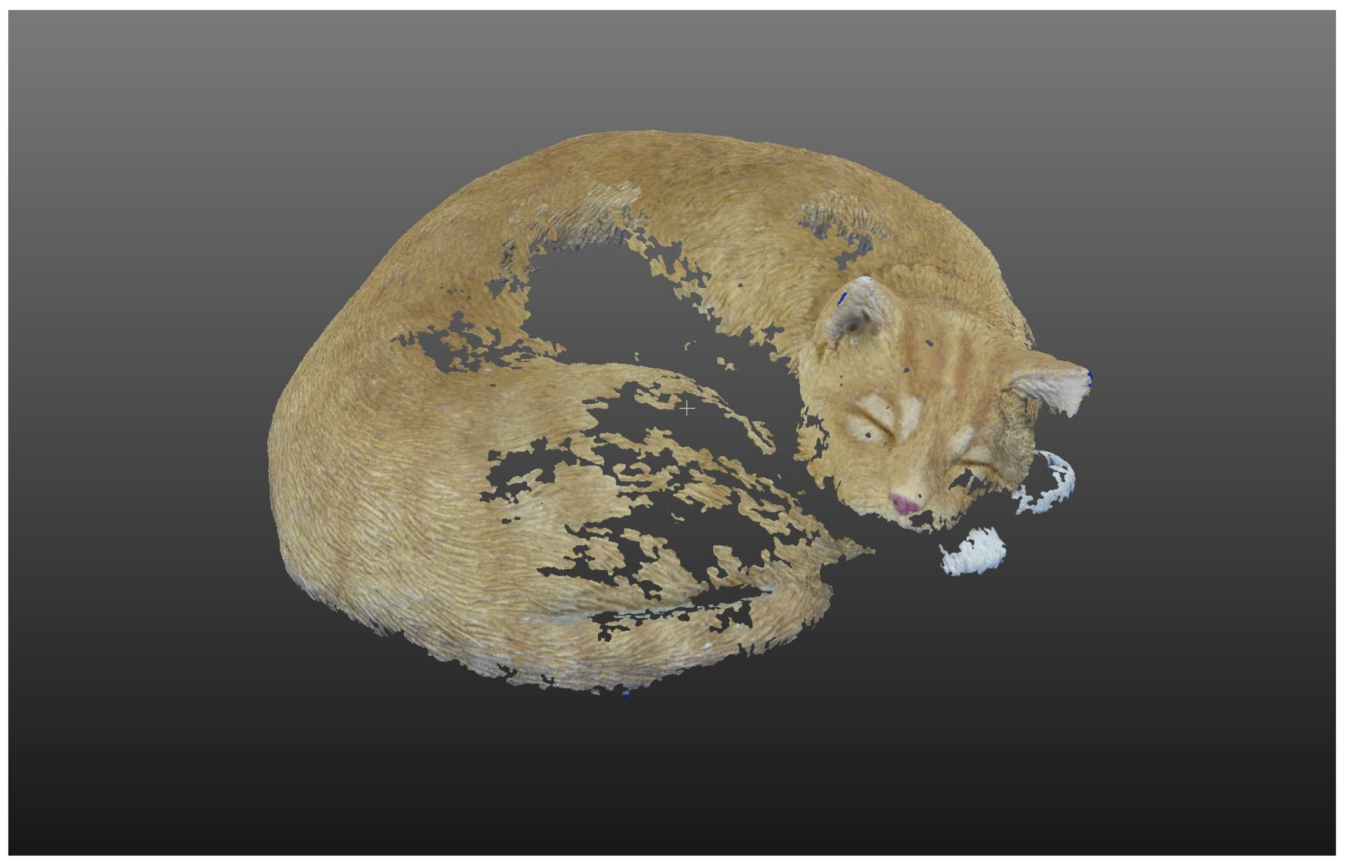
By manipulating these variables, it was possible to generate 60 different trials. Once the test trials were completed, the data from each trial were recorded. The output models were compared against each other for usability and computational time. Usability requires the model have enough points to build a mesh without having too many outlying points for it to cause interference. Examples of under-meshed and over-meshed are shown in
Figure 9 and
Figure 10, respectively.
5.1. Case 1: Results with the Benchmarking Dataset
After all of the models were run, the computational times were compared. The minimum time required to generate a model was 4.16 min, and the maximum time was 70.97 min. The trial information of most complete models is given in
Table 4. The results in
Figure 11 and
Figure 12 show that image count has a direct correlation with computational time. Results also revealed that with less than a certain number of photos, the model does not mesh. This was examined by trying to create a model using 18 photos and resulted in a failure to mesh. From
Figure 13, it can be seen that using the “Medium” setting requires approximately the same time to compile 36 photos as the “Low” setting takes for 108. This can be effective if the limiting factor is the number of photos available. There is also a subjective solution to what makes a model the “best”. In ideal circumstances, time is not an issue, and camera placement can be effectively controlled. However, in a real world implementation, the decision on what makes a model good enough could be entirely dependent on the time available. It is also of note that using too much data has a negative effect of adding too much noise to the model (
Figure 10).
Once an initial assessment of all of the models was performed, they were separated into several groups for comparison. For further analysis, the “best” model was selected. This was done by collecting all of the completed models together and then visually comparing them against each other for completeness with the fewest number of outliers. Through this comparison process, trial number 25 was determined to be the best model for this further investigation. Only selecting the best model was done visually considering outliers and completeness. However, after the initial selection, the model was compared against the laser scanned ground truth data provided with the dataset. The computational time for that trial was 18.56 min. The actual ground truth data were of a model that is roughly 300 mm from end-to-end at the widest part. Trial 25 generated 1,943,933 points with 97.02% of the values within 3 mm. This investigation provided enough information for a starting point for the next dataset. It also gives a good idea of what can be done to determine optimal number of photos to be used and most effective camera orientations. Furthermore, it should be noted that the design focus was to develop a rapid framework that could be used in minutes. For more detailed models, it is possible to improve the model and add a post-processing step, or even to run at a higher processing level to refine the model as desired. However, all those will increase the computational time. For instance, the image in
Figure 10 took nearly twice as long as the “best” model which was accurate within 1% and did not require post processing.
5.2. Case 2: Results with Custom Dataset
Once the benchmarking dataset was complete, a custom dataset was constructed for validation. To accomplish this, a trashcan with exactly 1-foot pieces of tape on it was used as the object to be reconstructed. The purpose of the tape on the trashcan was to create ground truth information. It was placed inside of a circle with a diameter of 10 feet and 32 equally spaced markings for camera placement.
Figure 14 depicts the circle and
Figure 15 depicts the placement of the trashcan.
To complete the dataset, 96 photos were taken from three different levels of 32 circumferential locations. The heights were set using a tripod and labeled low, middle, and high having settings of 1, 4, and 64, respectively. The photos were taken using a phone camera with 12MP resolution. For this dataset, a hardware improvement was made so that the trials could be run on all of the available COLMAP ”Quality” settings which included: “Low”, “Medium”, “High”, and “Extreme”. As the computational power of graphics card in System A became insufficient to run custom dataset cases, a different computer (System B) was used with the following specifications:
Intel Core i9-10850K CPU @ 3.60 GHz.
Ten physical cores with twenty logical processors.
128 Gb RAM.
Nvidia GeForce RTX3070 graphics card.
A similar process to the previous parameter analysis was used to evaluate the custom dataset. After all of the trials were completed, each model was evaluated for completeness. Having the ability to evaluate the COLMAP software with the custom dataset led to several new observations. With the “Cat” dataset, an “overmeshed” model resulted in outlier points that appeared where no object could be, as shown in the cat model (
Figure 10). For the custom dataset, an overmeshed model resulted in too much information generated far outside the area of interest; the reconstructed area ended up larger. For the custom dataset, the area of interest was the 10’ diameter circle that the trashcan was situated inside. A good example of this is depicted in
Figure 16.
Figure 17 depicts the overmeshed example where the modeled area was much too large, which resulted in the object being so overmeshed that the detail of the trashcan was diminished to just a rough cylindrical shape (
Figure 18). As more images were given to the system and run at a higher resolution, it allowed the algorithm to detect and match more features. This resulted in the meshed area becoming larger. The trashcan is an object that has a monocolor, symmetrical shape with few features. This results in a poor close up mesh of the trashcan when the area is overmeshed.
The area that is too large shown in
Figure 17 has a radius of roughly 75 ft, with the furthest objects being over 150 ft away. The observable meshed area has a direct relationship to the setting at which the software is being run. On the “Low” setting, the area is limited to immediate area regardless of how many images. This also holds true for the “Extreme” setting, where, regardless of how many images are used, the modeled area is very large. This only applies to the completed models. A list of trials that constructed a usable model are shown in
Table 5.
A comparison of the datasets revealed the most complete models were generated when the system was set to the highest possible settings. However, using all of the images in the dataset resulted in non-optimal models that were over-meshed with many outliers, as shown in
Figure 10,
Figure 17, and
Figure 18. Better models were generated when two levels of images were used, and all of the images on those levels were used. At lower settings, good models can be generated but require more images. For instance, 76 images were required to generate an “excellent” model on the “Low” setting, but only 36 images were required to generate a comparable model for the “Medium” setting for the “Cat” dataset. The best model for the custom dataset is shown in
Figure 19.
6. Validation Model Results
Using the components from the distributed behavior model and 3D reconstruction, the complete framework was established. A representation of the pipeline of the developed framework is depicted in
Figure 20. A confirmation implementation was designed to replicate a real world application. Given that the most robust models were constructed using images from two levels, two sUASs were used in the team. The two sUASs took off and move into the grouping phase. Once the entropy of the system fell below the threshold value of 0.1, the team moved into the mission phase and started its movement to the object of interest. When the team got closer to the object, they shifted into an orbit pattern, with one sUAS moving into a higher position and the other moving into a lower position, and started their orbit pattern. As the orbit began, so does the recording. A typical orbit took approximately 2 min and 10 s, and approximately 500 images were recorded.
AirSim provides the capability to take images from the perspective of the sUAS in the simulation environment. These are the images that were used in the reconstruction of the 3D model. The resolution of these images can be specified in the settings, and for the validation model experiments, they were set to 3840 × 2160 pixels. Images from the perspective of the sUAS are depicted in
Figure 21.
The 3D model of the object in interest, a house in these validation experiments, was constructed using 71 images from the dataset (
Figure 22).
Figure 22a depicts that the area around the house was limited to a reasonable area without the interference of multiple outliers. By limiting the area to a small radius, it is possible to generate better models and reduce the amount of time required to complete it. The reconstructed model has enough details; the ones that can be noticed are entry and exit locations, the chimney, and windows. Upon close inspection, the gutters can also be observed. It is clear enough that if a person, car, or animals were in the example, they could also be recorded. This provides confidence that the developed framework can perform well in real world applications. As presented in 3D reconstruction parameter analysis section, in the virtual world, it is more difficult to detect features because everything is perfectly simulated. In the real world, on the other hand, there are more features to detect, as presented in
Section 5.2.
The reconstruction of the model took 6 min 4 s from when the team completed their orbits. Looking at the total time spent, depending on where the sUASs were spawned, it could take up to 7 min for them to get through the grouping phase and then make their way to the objective. From there, they made an orbit, which took 2 min and 10 s. Modern off-the-shelf sUASs are capable of much faster physical operations that could accomplish this movement portion of the mission much faster. The tradeoff would be the time it takes to build the model, and it takes a little more than 6 min with the settings used in the simulations.
7. Discussions and Future Directions
In this paper, the aim was to present proof-of-concept results of the developed framework for rapid 3D reconstruction using distributed model-based multi-agent sUASs. There are several points that need to be addressed; those are worth mentioning here. In terms of distributed behavior model, the parameters should be tuned very carefully; otherwise, there might be cases of instability. One possibility is that sUASs may fail to group, and there are two ways that can happen; either the entropy threshold value is set too low, or the entropy is too high and the sUASs bypass the grouping phase all together. Another point that should be considered is that sUASs may have “edge characteristics”. That resulted in the entropy value being very close to the threshold value but not below the threshold, so one or more of the sUASs had an erratic path that resembled a wave pattern. This possible challenge was mostly solved by introducing sectors, described in
Section 3.2.
In terms of 3D reconstruction, it should be noted that the sUASs in the simulation environment each had one fixed camera. This makes it difficult to focus the cameras in the correct orientation so that it can look down at the object. When investigating the best camera poses, the best cases with just one angle were all done from the “Middle” or “High” positions where more of the object was in view in each image. In the cases where only perpendicular images were used, developed framework could not build a complete model. This limitation could be experienced in the simulation models; the “High” position also resulted in a much larger model radius. This is because when a sUAS is at the top of the roof of the house model, it needs to be in a position where the roof is in the bottom of the frame. When in this position, the rest of the image has a view out to the horizon. This results in poor models with huge model radii and many artifacts. Using a sUAS with a camera on a gimble would allow for maximizing the area in the field of view with the object of interest.
One immediate future work for this study will be to apply the framework using actual sUAS platforms in real world. Although parameter analysis in the real world with a fixed camera was presented, it is necessary to validate the results by using sUAS platforms. The goal of using fixed camera experiments is to eliminate all factors and a have controlled experiment to focus on proof-of-concept results of the developed framework. However, it is important to also test effects of real-world issues, such as vibration, coupled movement of the sUAS and camera, and motion blur, on the presented framework’s performance. That is why experiments with actual sUASs are planned for immediate future work of this study.
Additionally, the intent is to have all computations done by the onboard hardware of the sUAS. The simulation times recorded in the experiments were for a machine that is substantially better than the companion computers that could be placed on sUASs. However, given that comparative models can be established using lower resolution with more images, it is not likely that this would be much of an issue. Using twice or three times the images would not be a difficult adjustment to make given that most available off-the-shelf sUASs have high-resolution cameras mounted on them.
Another reason for plan future work with an actual platform is to see what kind of images are able to be recorded in different weather conditions. The simulation environment images were taken in a nearly motionless environment without wind, rain, platform vibration, glare, and several other uncertainties. Incorporating the framework onto a physical platform would undoubtedly bring up many challenges, some of which would likely be unforeseen. Integration onto hardware would also give a better estimate of mission completion time as well. The simulated sUASs are not designed to be high performance; as a result, the navigation time to the object in interest is the longest part of the process. This would not be the case when using an actual sUAS platform, and the mission completion time could be even shorter with relatively faster platforms.
8. Conclusions
In this study, a rapid 3D reconstruction framework was presented using structure from motion with images obtained from a team of sUAS. Details of the distributed behavior model for a team of sUASs and 3D reconstruction steps were provided. For the distributed behavior model that is based on the entropy of the system, a parameter analysis was conducted with the intent of having a robust and scalable algorithm capable of navigating the sUASs to the desired positions. Parameters used for evaluation were (i) minimum distance between sUASs and (ii) entropy threshold. Simulations were run with various numbers of sUASs to confirm scalability, robustness, and threshold values. A minimum distance setting was confirmed, and a function for scaling the threshold value was determined. For the 3D reconstruction step, COLMAP was evaluated with two separate datasets for optimization with the intent of reducing the computational time required to build a model that is usable. One dataset was a controlled environment for initial analysis, and the other dataset was of a real world environment for applicability to hardware implementation. The priorities are usability of the model and speed of reconstruction. During this evaluation, four parameters were analyzed in software for evaluation: quality, image number, camera angle, and multiview formation. As a validation experiment, a team of two sUASs was able to use the entropy-based distributed behavior model to take off from different locations and then group together in the simulation environment. Then, they made their way towards a predefined object and recorded images of the object while in orbit. Once the orbit was complete, the total of 71 images, which were separated by approximately 10 degrees and from two levels, were used to reconstruct the model, and a rapid model could be constructed in low resolution in as little as 6 min 4 s from when the team completed their orbit motion. This would be helpful in emergency situations, such as wildfires, disaster relief efforts, and search and rescue missions. In those situations, an in-depth, highly accurate model is not necessarily required, but a rapid solution could be crucial. The planned future work included transitioning the framework onto real hardware systems.


