Abstract
In robotics and automated manufacturing, motion functions for parts of machines need to be designed. Many proposals for the shape of such functions can be found in the literature. Very often, time efficiency is a major criterion for evaluating the suitability for a given task. If there are higher precision requirements, the reduction in vibration also plays a major role. In this case, motion functions should have a continuous jerk function but still be as fast as possible within the limits of kinematic restrictions. The currently available motion designs all include assumptions that facilitate the computation but are unnecessary and lead to slower functions. In this contribution, we drop these assumptions and provide an algorithm for computing a jerk-continuous fifteen segment profile with arbitrary initial and final velocities where given kinematic restrictions are met. We proceed by going systematically through the design space using the concept of a varying intermediate velocity and identify critical velocities and jerks where one has to switch models. The systematic approach guarantees that all possible situations are covered. We implemented and validated the model using a huge number of random configurations in Matlab, and we show that the algorithm is fast enough for online trajectory generation. Examples illustrate the improvement in time efficiency compared to existing approaches for a wide range of configurations where the maximum velocity is not held over a period of time. We conclude that faster motion functions are possible at the price of an increase in complexity, yet which is still manageable.
1. Introduction
Moving quickly from one motion state (position, velocity, acceleration, …) to another one is essential for efficiency and quick reactions to unforeseen events in robotics as well as in other areas such as automated manufacturing machines [1,2,3]. This has led to numerous suggestions of motion functions that take into account restrictions on velocity, acceleration and even higher-order derivatives [1]. The meanwhile classical approach using a “bang-zero-bang” discontinuous acceleration profile, which switches from maximum to zero to minimum constant values, turned out to be unsuitable in many cases, since it cannot be realized by controllers and induces unwanted vibrations. Therefore, very often, motion functions are required to have at least a continuous acceleration. An algorithm for computing such a function with piecewise constant jerk (”seven segment profile”) was presented by the author in [4], where restrictions on velocity, acceleration, and jerk and boundary conditions regarding velocity and acceleration can be prescribed. If there are stronger requirements on vibration reduction (e.g., for restricting position errors), higher-order continuity of the motion function has proven to be effective in experimental settings [5,6,7,8,9,10,11,12]. In this contribution, we present an algorithm for computing a jerk-continuous motion function (as opposed to the piecewise-constant, discontinuous jerk function designed in [4]) in one dimension, such that symmetric restrictions regarding velocity, acceleration, jerk, and snap (the derivative of the jerk, abbreviated as sn in the sequel) are fulfilled and boundary conditions for position and velocity can be arbitrarily prescribed. We term this function as “fast” because, at any time, for at least one of the kinematic restrictions, the maximum or minimum is reached. Moreover, we show that the algorithm for computing this function is fast enough for online trajectory generation where a computation should be performed within a controller cycle [13,14].
Since the task of designing a fast motion function is so elementary, a considerable number of research articles have appeared, particularly in the last two decades. This work can roughly be organized into two classes: in the first one, the task has been formulated as a restricted optimization problem, and algorithms from this field have been applied (e.g., [15,16,17,18,19,20,21,22,23,24,25]). This approach has the advantage that other aspects such as position errors regarding a given path or energy consumption can be easily included, and even a multi-objective optimization can be performed [22]. Moreover, optimization approaches often employ quintic spline functions, which guarantees continuity up to the snap function (fourth derivative). Yet, for online trajectory generation, the optimization algorithms are too slow. Only the contribution by Valente et al. [18] reports a sufficiently fast optimization procedure, but their three-segment profile could also be computed directly and leaves much space for improving on time efficiency. This leads to a second kind of approach, which construct the motion function directly based on the given restrictions and boundary conditions. For the subsequent literature overview, we restrict ourselves to those approaches which design a jerk-continuous motion function where restrictions at least regarding velocity, acceleration and jerk can be prescribed [11,12,26,27,28,29,30,31,32,33,34].
In order to provide a well-structured overview, we apply the following criteria in our description: we first consider the kind of task regarding the boundary conditions of the motion. In many tasks, point-to-point motions are to be designed (e.g., in pick-and-place tasks) where initial and final velocities and accelerations are zero. These are also called rest-to-rest motions and are abbreviated as RR in Table 1. In automated manufacturing, one often has a situation where initial and final velocities are given and higher-order derivatives are zero (cf. [17,35,36]), e.g., when a tool moves with constant velocity for performing a certain task and then has to quickly move to another place to again perform a task with constant velocity. Using an abbreviation from a guideline of the German Association of Engineers [37], we term this task GG in Table 1 (for more information on the tasks, see [4]). Note that the task GG comprises the task RR, since the velocities are allowed to be zero. In robotics, there are also situations where the initial and final velocities and accelerations are arbitrary, e.g., when one has to react to unforeseen events (see [13]). This kind of task is abbreviated as BB in Table 1, where BB+ denotes that higher-order derivatives greater than 2 can also be prescribed. Again, the task BB contains the task GG. As can be seen in Table 1, most of the recent articles are restricted to RR, since this task can become already quite complicated when a fast motion function using the limitations as far as possible is required. The second criterion consists of the type of jerk function. Many of the designed functions in Table 1 work with a fifteen-segment approach, which is the natural extension of the seven-segment profile for motion functions with continuous acceleration. Some authors [11,27,34] also allow more generally for segments when restrictions up to the n-th derivative are to be taken into account. Other approaches achieve smoother jerk functions using trigonometric and zero pieces (having less discontinuities in the snap), but this restricts the possibilities to stay at the maximum value for some period of time. The next criterion is the continuity level of the motion function, i.e., up to which derivative continuity is guaranteed. All functions considered in this summary are required to be at least jerk-continuous, i.e., the continuity level must be at least 3. As can be seen from Table 1, most of the reviewed articles guarantee just the minimum order of 3. In the functions proposed by Lee and Choi [29] and Nguyen et al. [27] (part b), the snap is also continuous, which, on the other hand, has the disadvantage of a slower motion. In the approach by Ezair et al. [34], Nguyen et al. [27] (part a) and Biagiotti and Melchiorri [11,33], the continuity order can be freely chosen (we denote this by adding a “+” in Table 1), but orders higher than 3 lead to an increase in computational effort, which can make the suitability for online trajectory generation questionable. Fang et al. [30] propose the sigmoid function for going from one constant segment to another one, where all derivatives are continuous. Again, this leads to slower motion functions, as there is always a tradeoff between smoothness and time efficiency. The next criterion is concerned with the kind of kinematic restrictions that can be taken into account. As stated above, we only consider proposals where restrictions on velocity, acceleration and jerk can be guaranteed. Only the designs that work with fifteen segments using linear pieces (or the sigmoid function) also allow us to prescribe a restriction on the snap. This way, it is possible to avoid jerk functions that are “theoretically” continuous but have such a steep increase in jerk that the intended property of vibration reduction is not achieved. In the proposals by Ezair et al. [34], Nguyen et al. [27] (part a) and Biagiotti and Melchiorri [11], one can choose up to which derivative restrictions can be described (denoted by a “+” in Table 1).

Table 1.
Jerk-Continuous Motion Functions with Restrictions.
The final two criteria deal with the question of whether the proposed shape or algorithm affects the time optimality of the motion function. The first one states for which kinematic functions periods of constant maximum or minimum value are possible. If this is not the case, the resulting functions are often sub-optimal because they do not take full advantage of the given restrictions. Only the designs working with a piecewise linear function with fifteen segments (or more) provide the possibility of having constant phases for maximum/minimum velocity, acceleration, jerk and snap. If there are only three segments as in Wang et al. [31], only the velocity can be held at a constant extremal value. Secondly, there are assumptions in nearly all proposals that are often implicit in the jerk functions and are only seldom stated explicitly. Biagiotti and Melchiorri [1] point out that the provided formulae are only valid when all extremal values (for v, a, j) are taken (this requires a minimum distance to be travelled). In the function proposed by Fang et al. [29], the extremal jerk must occur, which, again, is not necessary for small distances. All but one of the approaches include an assumption that is recognized as making the function potentially sub-optimal by Ezair et al. [34] and Biagiotti and Melchiorri [11]: they assume that when the velocity reaches its extremum in the middle piece (in functions with fifteen segments, this is segment eight), the jerk goes back to zero. This is only necessary when the extremum is the maximum/minimum possible velocity, and this is held for a time period of length greater than zero. If the distances to be travelled are not so large that this is the case, then the assumption leads to an avoidable loss in time efficiency. In the approaches by Fang et al. [30], Nguyen et al. [27] (part b) and Lee and Choi [29], additionally, the shape of the function requires the snap to be zero when the extremum of the acceleration is reached, which is also unnecessary. Moreover, this applies to higher-order derivatives in Ezair et al. [34] and Nguyen et al. 2008 a [27]. The reason for making this assumption is quite obvious: it leads to a mathematically better tractable problem with manageable complexity. Only in the approach by Biagiotti and Melchiorri [19] (in the task RR) is a way to remedy this problem suggested by staying at the maximum/minimum jerk level, but we will give an example showing that, still, their algorithm includes assumptions that prevent them from finding a time-optimal solution in several configurations.
The design presented in this contribution improves what can be found in the literature in the following ways:
- We design a jerk-continuous motion function with better time efficiency by avoiding any additional assumption, particularly that the jerk must go down to zero at the intermediate extremal velocity. This improves the currently available approaches relating to the rest-to-rest (RR) task as well as the work on the GG task (arbitrary initial and final velocities). Using randomly generated input data (restrictions, distance, initial and final velocities), we demonstrate that there are a variety of different possible configurations, and hence we show that the task has an inherent level of complexity that cannot be sidestepped without staying sub-optimal in some situations. Therefore, one cannot expect that simple algorithms will optimally cover all situations.
- The algorithm presented in this contribution is also computationally efficient and hence suitable for Online Trajectory Generation (OLG), which is needed to quickly react to unforeseen events in human–robot interactions.
We do not term our approach “optimal” because we do not have mathematical proof for this (for such kinds of proof see [28,34] where, for example, in [28] the proof is performed by assuming that there is a motion function needing less time, which leads to a contradiction based on a theorem from the field of differential equations; the proof depends on the additional assumption that the jerk is zero at an intermediate velocity). Since, at any time, at least one restriction is adopted, we term our function “fast”.
Our approach has two main areas of real-world application: first, to improve on time efficiency and hence throughput in automated production and, at the same time, to control vibrations and positioning errors by guaranteeing jerk continuity and restriction; secondly, to allow for quick reaction in case of unforeseen events in robotics, particularly when human interaction is involved and computing a new motion function must be performed within a controller cycle (cf. [13,25]).
The paper is structured as follows: Section 2 provides some basic concepts and visualizations that guide our work, and we split the task into two major cases depending on whether or not the maximum jerk can be reached before the maximum acceleration (the distinction is already made in Fan et al. [28]). In Section 3 and Section 4, the motion models that can occur in cases I and II are stated, and criteria for switching between models are investigated depending on the intermediate critical velocities and jerk values being reached. In Section 5, we outline our algorithm for setting up the fifteen-segment profile by finding the suitable model. We present our implementation in Matlab®, which we validated using a huge number of randomly chosen tasks. Stability and time efficiency aspects important for online trajectory generation are discussed. In Section 6, we compare our results with those of Fan et al. [28], Ezair et al. [34] and Biagiotti and Melchiorri [11] by presenting some numerical experiments in example configurations. Section 7 summarizes the results, highlights the improvements and outlines directions of future work. All formulae and algorithms needed to reproduce our work have been placed in the appendices.
2. Basic Concepts and Situations
This contribution is concerned with finding a fast jerk-continuous motion function when the following six values are given: , , , (each >0) such that ,,,; initial velocity: ; final velocity: ; distance: Δs (arbitrary real numbers). Initial and final accelerations and jerks are assumed to be zero. Without loss of generality, we only consider the case , since otherwise, we can simply change the positive direction of the distance. We solved this task using a fifteen-segment profile, as shown in Figure 1, for the rest-to-rest (RR) situation. Note that all fifteen segments are only needed when the maximum and minimum jerk, acceleration and velocity values are taken for a time period of length larger than zero.
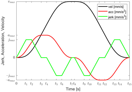
Figure 1.
Fifteen-segment motion profile.
Broquere et al. [38] introduced the so-called velocity-acceleration plane to visualize seven-segment motion functions. This visualization has proved to be very helpful in [4] in order to systematically go through the space of all possible situations. In this contribution, we proceed analogously, but the plane has more structure to it. Figure 2a depicts the area of the plane within which a motion can be placed as a parametric curve . The boundary curve consists of pieces where the extremal values of snap, jerk and acceleration, respectively, are taken. We apply the following color coding: light blue, light green and light red denote the maximum values of snap, jerk and acceleration, respectively. The “dark” versions of the colors denote the minimum values. In order to avoid over-coloring, we draw the boundary curve in black and only apply the color coding for the parametric motion curves. This can be seen in Figure 2b, where an example curve is displayed, which has only nine segments. Such a curve must run from left to right through the upper half-plane and from right to left through the lower one. Note that the parametric curves do not have any kinks, as is the case for only acceleration–continuous motion functions with piecewise constant jerk, as considered in [4,38].
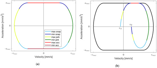
Figure 2.
Velocity-acceleration plane. (a) Boundary curve; (b) parametric motion curve.
As is conducted in [28], we distinguish between two major cases depending on whether or not the maximum jerk is reached when applying the maximum and minimum snap in order to get from acceleration zero to maximal acceleration. For the convenience of the reader, we briefly summarize some of the results developed in [28]. The maximum jerk is not reached (Case I) if and only if holds. We term the other case as Case II in the sequel. We describe a point in the velocity–acceleration plane by a triple , where the third “coordinate” provides the jerk value of the point . A straightforward computation (cf. [28]) yields the time needed for going from to in the velocity–acceleration plane by accelerating and decelerating as much as possible (see Figure 3a), abbreviated as . The results need further sub-cases and are given in Table 2.
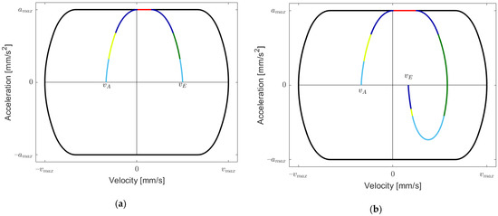
Figure 3.
Parametric motion curves. (a) Going from directly to ; (b) going from to and back to .
Table 2.
Results by Fan et al. [28].
Using the durations stated in Table 2, the distance for going directly from to can simply be computed as:
In [28], this consideration is actually sufficient, since it is assumed that when the velocity reaches its extremal value , then the jerk goes back to zero, such that the overall motion can be split up into two parts, from to and from to . This is depicted in Figure 3b.
Our basic idea is also to work with an intermediate extremal velocity , but we obtain a shorter time (in cases where the maximum velocity is not taken for a non-zero period) by allowing the jerk to be non-zero. We will provide an example in Section 6. We first restrict ourselves to the situation where the required distance Δs is greater than or equal to . For finding a suitable intermediate velocity, we let move from to . We choose the corresponding jerk value by finding the lowest (negative) value such that it is possible to get back from to using extremal snap. Figure 4a shows the jerk function with three time intervals of lengths , and . This function must fulfill the two requirements: and . Since the snap is maximal on the first interval, we obtain
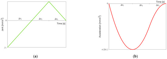
Figure 4.
Function for going back. (a) Jerk (b) Acceleration.
From the first requirement, it follows that , and hence
Now, we consider , as shown in Figure 4b. Since for , we have , we obtain
Now, we consider . For , we have , and hence
From the second requirement, we obtain . By substituting according to Equations (2)–(5), we finally obtain
From Equation (6), we can also easily compute the intermediate velocity for which reaches , which is . Note that this might be larger than , but we neglect this for the moment. We now define the function vm2jm, which maps to the corresponding jerk value :
The main reasoning behind our method can be summarized as follows:
- In order to cover all possible distances larger than or equal to , we let the intermediate velocity and corresponding jerk “flow” from via to where might become constantly at some intermediate velocity. Then, we proceed further by going from to . From there, one can achieve arbitrarily large distances by moving constantly with . Since in this “flow”, we make continuous changes in and , the covered distances also change continuously, and thus we have full coverage of all distances . One can proceed in a similar way by letting run from to , covering all distances .
- In this “flow”, we identify the occurring jerk models and the switching points when there is a model change. For this, we compute the so-called “critical” velocities and jerks where extremal values of acceleration or jerk are reached.
- For all velocity-jerk combinations where there is a model change, we compute the distances reached such that we can determine which model must be applied for the given distance. In that model, we then can compute the time periods of the segments it consists of.
The subsequent Section 3 and Section 4 describe the occurring models, the computation of “critical” velocities and jerks as well as model sequences when traversing the velocity-acceleration plane. In Section 5, we describe how to compute the time periods in the applicable model using a simple bisection method.
3. Models and Critical Velocities and Jerks in Case I
In Case I, is not reached when going from to the maximal acceleration where the jerk must be zero. The maximal possible jerk value occurs when starting at a point with and applying maximal snap until one reaches . A simple computation yields the value . If is larger than this value, we simply set .
We first assume , and we neglect the restriction on maximal velocity. In order to manage complexity, we split the task of finding suitable models into two parts: going “forth” from to and going “back” from to . Figure 5 shows possible jerk models for going “forth” using maximal, minimal or zero snap (the notation “I.xf” refers to these models in Case I). The first four models are built using the criteria of whether is or is not reached when going from the maximal acceleration (of this function) down to acceleration zero, and is or is not reached. Model I.1f depicts the situation where and are both not reached. Model I.2f shows the motion going “forth” when is reached but is not reached, whereas Model I.3f is vice versa. In Model I.4f, both and are reached. In both models I.2f and I.4f where is reached, still holds, which need not be the case. As in Model I.2f, in Model I.5f is reached and is still not reached, but now, . Finally, in Model I.6f, both and are reached (as in Model I.4f), and . Note that Models I.5f and I.6f could also be treated as special cases of Models I.2f resp. I.4f with resp. . We decided to set up separate models for two reasons: reaching certain limits (here ) is more recognizable by having a model change, and the models can then be simpler (see the formulae in Table A1).
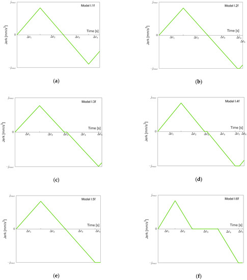
Figure 5.
Jerk models in Case I going forth. (a) , not reached; (b) reached, not reached, ; (c) not reached, reached; (d) , reached, ; (e) reached, not reached, ; (f) , reached, .
If one of these models is suitable for going from to (conditions for this are investigated below), one has to compute the length of the time intervals (I = 1…4 or 5 or 6). In order to have a simple notation in the subsequent computations, we define the point in time () as . From the jerk models, one can easily produce acceleration and velocity models using the initial values 0 and , respectively. We have three conditions that must be fulfilled ( denotes the sum of the time intervals):
Further conditions originate from the special shape of the model functions: In all models we have ; additional equations can be set up when or are reached. It is easy to check that this results in a sufficient number of equations for computing the time intervals. These equations lead either directly to formulae for the time intervals or to a polynomial equation that has a time interval as one of its roots. We demonstrate this for Model I.1f, where the equations to be fulfilled are the following:
From , we obtain , and hence
From , it follows that
By integrating the jerk function twice and using , one obtains:
By substituting and in Equation (13) using Equations (11) and (12), we obtain an equation where only is unknown. This equation cannot be solved analytically, and because of the square root in Equation (11), it is not a polynomial equation. Yet, using algebraic transformations, it can be turned into a polynomial equation of degree 6, the solutions of which have to be multiplied with . We used the Computer Algebra System (CAS) Maple® for doing this. The coefficients of the polynomial are given in Appendix A (Table A1, Model I.1f). Note that all solutions to the original Equation (13) are also solutions to the transformed polynomial problem but not the other way around, such that it must be checked which of the solutions solve the original problem. Nonetheless, by transforming the problem into a polynomial one, stable polynomial solvers can be employed, which find all roots such that one can avoid the problem of depending on suitable initial values in order to find feasible solutions. This strategy has been pursued at several places in our algorithms, and all resulting polynomials can be found in the appendices.
In all other models in Case I “going forth”, we similarly get the respective equations but those can be solved directly where again a CAS is helpful. Sometimes, one obtains more than one solution, but it is always possible to find among those the only one that provides a real positive value. The results are shown in Table A1 (Appendix A).
Figure 6 depicts the possible models for going “back” from to . Clearly, before (or at the same moment as) the acceleration goes down to , the jerk reaches its minimal value . Therefore, we have a simple sequence of the three models I.1b, I.2b and I.3b, as shown in Figure 6a–c when we proceed from to . Note that not all models must be present depending on the value of . When we then proceed from to , as described in the previous section, one of the Models I.4b to I.7b might occur (Figure 6d–g). Models I.4b, I.5b and I.7b simply add a “front piece” starting at , which goes up to zero. Model I.6b is needed, since when starting with Model I.7b and reducing , it is possible that first, the minimal jerk becomes larger than before the minimal acceleration becomes larger than . Note that when reaching , the model must be symmetric, since one starts and ends with acceleration zero. Again, one could treat Models I.1b, I.2b and I.3b as special cases of Models I.4b, I.5b and I.7b with , but, for the same reasons as stated above, for going forth, we treat them separately. From the jerk models, one can easily produce acceleration and velocity models using the initial values 0 and , respectively. We have three conditions that must be fulfilled ( denotes the sum of the time intervals):
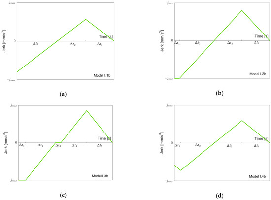
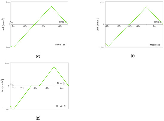
Figure 6.
Jerk models in Case I going back. (a) ; (b) , not reached; (c) , reached; (d) , , not reached; (e) , reached, not reached; (f) , not reached, reached; (g) , , reached.
Further conditions originate from the special shape of the model functions: in all models, the final two time intervals must have equal length. Moreover, in Models I.2b, I.3b, I.5b and I.7b, there is an interval where the jerk goes from its minimum to zero. In Models I.3b, I.6b and I.7b, the minimal acceleration is reached. Finally, there is a relation between the start jerk and the first two resp. three time intervals in Models I.4b, I.6b resp. I.5b, I.7b (note that in Model I.1b, and are related via Equation (8), upper part, so the system of equations is not overdetermined). It is easy to check that this leads to a sufficient number of conditions to determine the time intervals in all models going “back”. The corresponding equations lead either directly to formulae for the time intervals or to a polynomial equation of a degree of at most four, which has a time interval as one of its roots (cf. the exemplary computation of time intervals for the “going forth” model I.1f above). We provide the respective expressions in Appendix A, Table A2.
Next, we address the question in which possible sequences the models occur when runs from to , as stated in the previous section. For this, we investigate the values of for which, in the going forth situation, the minimal jerk reaches the value (denoted by ), and the maximal acceleration reaches the value (denoted by ). In the sequel, we present the procedure for which the algorithm can be found in Appendix B, Algorithm A1.
- If the inequality holds (cf. Table 1), then is already reached for , so we have . In order to find , we set in Model I.3f. In the equations given for the time intervals in Appendix A, Table A1, for this model, now, is unknown, but the additional equation allows us to compute this quantity: since , , and , we obtain the formula presented in line 3 for . The corresponding value for can be determined using Equation (6). This gives , and we are done.
- Otherwise, we consider Model I.1f and investigate the condition , i.e., . Again, is an additional unknown. If , we have because of symmetry. Otherwise, by substituting and in Equation (13) using Equations (11) and (12), we obtain an equation where, now, only is unknown. This equation can be transformed into a polynomial one of degree 6, the coefficients of which are given in line 8 of algorithm A1. We pick the real root for which holds.
- Next, we have to check whether is really reached before . For this, we compute in Model I.1f, which gives , and we check whether holds. If that is the case, then is reached first, and we compute according to Equation (6) (cf. line 14). Then, we set in Model I.2f. This leads to the formula for presented in line 15. If , then Model I.2f was applicable, and we obtain according to Equation (6), as presented in line 17. Otherwise, we have to apply Model I.5f (i.e., has already reached ), and we obtain according to line 18.
- Otherwise (i.e., ), is reached first, and we have to set in Model I.1f. This additional equation allows us to compute as the real root of the polynomial of degree 4 presented in line 21, for which holds. Then, again, we obtain according to Equation (6), as given in line 23. By setting in Model I.3f, we obtain the value for when is reached, and line 25 computes the corresponding value for .
The algorithm illustrates a strategy often pursued in this work: By going stepwise through the available models one ends up with an applicable model in which one can compute the desired value either directly or by computing roots of a polynomial.
Note that “critical” velocities might be larger than . We will look at the possible configurations below. Next, we investigate at which value of in the going “back” part the minimal jerk and the minimal acceleration are reached (denoted by and by , resp.). In the “going back” situation, we always have , and we obtain using Equation (6) with and by setting in Model I.2b (see Table A5).) Figure 7 depicts the possible relative positionings of , and on the -scale and provides information on which model to apply when lies within a certain interval left of . In Figure 7b,d,e, Models I5.f resp. I.6f have to be chosen once is reached. Note that the interval of possible values for starts at and ends at , so if, for example, in Figure 7c or e, then Model I.1f does not occur.
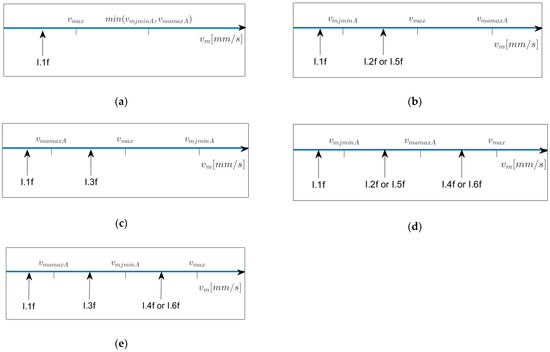
Figure 7.
Relative positioning of , and on the scale and corresponding models.
Figure 8 depicts the possible relative positionings of , and on the scale and provides information on which model to apply when lies within a certain interval left of .
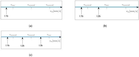
Figure 8.
Relative positioning of , , and on the -scale and corresponding models.
So, we are able to specify the applicable model when runs from from to in Case I. The remaining task consists of finding the correct model when we go from to , i.e., we keep constant and let run from to 0. The additional challenge here originates from the possibility that already-reached extremal values , (for going forth) resp. , (for going back) might be no longer reached. For example, when was reached (going forth) and moves to zero again then, at some value of , the minimal jerk has to be above since we are in Case I. Figure 9 demonstrates this in the velocity acceleration plane where we omit the boundary curve for better visibility of interesting curve sections: we have for the restrictions, , and , resulting in a distance (in our examples, the units are always , , , and , respectively, and we omit these in the sequel for brevity). We recognize Model I.6f for going forth and I.2b for going back in Figure 9a,b. When we now enlarge to , we obtain a distance of 167, and we see in Figure 9c that the models switched to I.4f and I.4b, respectively. When we now consider the final jerk value zero, we obtain as distance 201.19, and Figure 9d shows that the going forth model again switched to I.3f, whereas the going back model does not change. The three curves in Figure 9b–d are close to each other, but by zooming, we see that we obtain higher curvature when moving to . In this case, the maximal acceleration is still reached, but when one moves closer to such that the part with constant acceleration is very short, another model switch might occur. This illustrates the inherent complexity, which cannot simply be sidestepped.
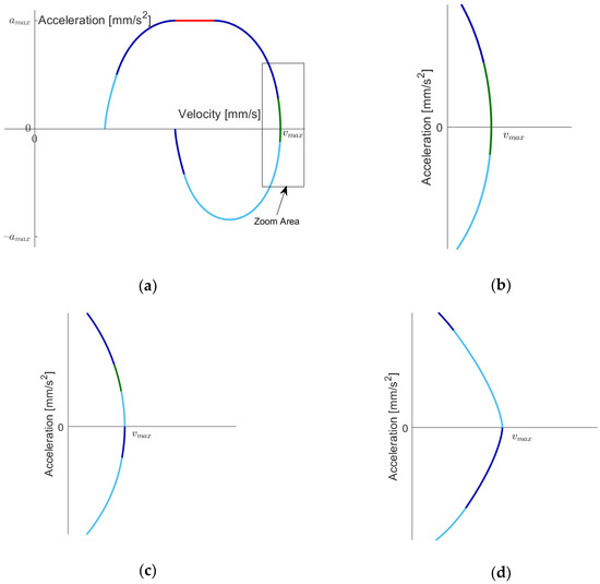
Figure 9.
Going from to . (a) ; (b) zoom into (a); (c) zoom into ; (d) zoom into .
Next, we find out at which values for certain model switches occur. We set and proceed similarly as when determining the critical velocities: in the models, we add an additional equation depending on which extremal acceleration or jerk has been reached, and we determine as an additional unknown; the latter can be computed directly or via solving a polynomial equation. If the solution leads to non-admissible values for or to negative values for time intervals, then there is no feasible solution. Since the computations are straightforward and can be easily performed using a CAS, we just give the results that are needed for implementation. The procedure is described in more detail in Algorithm A3. We first consider the going forth part and refer to Figure 7 regarding the possible positionings of . If we have situation (a), Model I.1f will be applied for all jerk values. If situation (b) applies, we proceed as follows:
- In Model I.1f, set and and compute by proceeding as stated in Algorithm A3, line 2, denoted by . There must be a solution, since we must end up with a symmetric model, and Model I.2f is not symmetric.
- For , apply Model I.2f, for Model I.1f.
If situation (c) applies, the procedure is as follows:
- In Model I.1f, set and and compute by proceeding as stated in Algorithm A3, line 5, denoted by in case of existence. If there is no such solution, the suitable model is always Model I.3f. This is also the case when holds (cf. the explanation for Figure 5).
- Otherwise, for , apply Model I.3f, for Model I.1f.
If situation (d) applies, perform the following:
- In Model I.4f, set and (i.e., the phase of constant minimal jerk has duration zero). Compute and substitute the value into the expression given for in Table A1, Model I.4f. If holds (i.e., the solution is admissible), set , and the next model is I.3f. Otherwise, set in Model I.4f (i.e., the phase of constant maximal acceleration has duration zero) and compute by proceeding as stated in Algorithm A3, lines 12/13, also denoted by . If there is a real solution with , the next model is I.2f. Since Model I.4f is not symmetric, a valid must exist.
- If Model I.3f is next, set and in Model I.1f and compute as in situation (c), denoted by . This need not exist.
- If Model I.2f is next, set and in Model I.1f and compute as in situation (b), denoted by . This, then, must exist, since I.2f is not symmetric.
- Now, for , take Model I.4f. For , apply Model I.3f or I.2f, resp. If no valid exists, apply Model I.3f for . Otherwise, for , Model I.1f is suitable.
Finally, if situation (e) applies, we have the same procedure as for situation (d). If , there is no and we switch directly from Model I.4f to I.3f.
Next, we consider the going back situation and refer to Figure 8. If we have situation (a), Model I.4b will be used for all jerk values. If situation (b) applies, we proceed as follows:
- In Model I.5b, set and and compute , denoted by by proceeding as stated in Algorithm A4, line 2. There must be a solution, since we must end up with a symmetric model, and Model I.5b is not symmetric.
- For , apply Model I.5b; for , Model I.4b.
If situation (c) applies, perform the following:
- In Model I.7b, set and (i.e., the phase of constant minimal jerk has duration zero), and compute according to Table A2. Substitute the value in the formula given for (Model I.7b), and check if . If this is the case, set , and the next model is I.6b. Otherwise, set in Model I.7b (i.e., the phase of constant maximal acceleration has duration zero), and compute according to Algorithm A4, line 10, also denoted by . If there is a real solution, the next model is I.5b. Since Model I.7b is not symmetric, a valid must exist.
- If Model I.6b is next, set and , and compute according to Algorithm A4, line 15, denoted by . This need not exist.
- If Model I.5b is next, set and , and compute according to Algorithm A4, line 2, denoted by . This, then, must exist, since I.5b is not symmetric.
- Now, for , take Model I.7b. For , apply Model I.6b or I.5b, resp. If no valid exists, apply Model I.6b for . Otherwise, for , Model I.4b is suitable.
Now, for all triples , we can determine the model to be applied in Case I when holds. Moreover, one can stay at for a period of arbitrary length, which can easily be included between the going back and the going forth part.
When , we can take intermediate velocities that lie left of , and by reflection and reversion, we can rewrite the problem as one where : Assume, (still with ), and are given where holds. Then, consider the reflected configuration (denoted by a bar): , , and . Since , we can perform the procedure explained above. Then, we reverse the solution by reflecting it again, i.e., we consider
Figure 10 illustrates this (we omit the boundary and color coding for simplicity reasons). The left magenta part shows the solution to the reflected problem, and then by reflection (and thus reversion), we obtain the solution to the original problem in black. Thus, we cover all possible distances.

Figure 10.
Reflection of the problem and of the solution to the reflected problem.
4. Models and Critical Velocities and Jerks in Case II
In Case II, we proceed analogously to Case I. Again, we take an intermediate velocity and a corresponding jerk and go “forth” from to and “back” from to . Figure 11 shows possible jerk models for going “forth” (the notation “II.xf” describes these models in Case II) using maximal, minimal or zero snap. In Case II, there are three interesting switching points: is reached when going down from the maximal acceleration; resp. is reached when going up from . Note that Models II.1f, II.2f and II.3f are identical to Models I.1f, I.2f and I.5f. In the other models, the maximum jerk is reached, which is not possible in Case I.
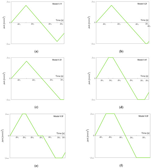
Figure 11.
Jerk models in Case II going forth. (a) , and not reached; (b) reached, not reached, ; (c) reached, not reached, ; (d) and reached, ; not reached; (e) , and reached, ; (f) and reached, not reached; . (g) , and reached, .
If one of these models is suitable for going from to , one has to compute the length of the time intervals (I = 1…4, 5, 6 or 7). Again, the conditions stated in Equation (9) for Case I carry over to Case II. Further conditions can be identified by looking at the special shape of a jerk model. If an interval starts or ends at or , it has to have a length . In Models II.1f, II.2f and II.3f, the first two intervals have the same length. Moreover, in Models II.5f and II.7f, . It is easy to check that these conditions provide the required number of equations for determining the in the respective model. The results are given in Appendix A, Table A3.
Figure 12 depicts the possible models for going “back” from to in Case II. Models II.1b and II.2b are identical to I.1b resp. I.2b. In Model II.3b, is reached, and finally, is reached in Model II.4b. We have a simple sequence of the four models, as shown in Figure 12a–d, when we proceed from to . Note that not all models must be present depending on the value of . When we then go further from to , one of the Models II.5b to II.8b might occur (Figure 6e–h). These models simply add a “front piece” starting at . When reaching , the model must be symmetric.
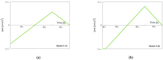
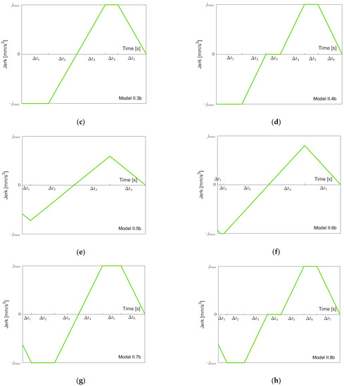
Figure 12.
Jerk models in Case II going back. (a) ; (b) , not reached; (c) , reached, not reached; (d) , and reached; (e) , , not reached; (f) , reached, not reached; (g) , and reached, not reached; (h) , , and reached.
For computing the length of the time intervals, as in Case I, Equation (14) provides some conditions. Further necessary conditions can be derived similarly, as stated for the going forth part in a straightforward manner, so we omit this. The results are given in Appendix A, Table A4.
Next, we address the question of in which possible sequences these models occur when runs from to . For this, we consider the critical velocities starting with the going forth situation. The value of for which the minimal jerk reaches the value is denoted by ; the value for which the maximal jerk reaches is denoted by . Moreover, the intermediate velocity at which is reached is called . Case II is simpler than Case I in that we always have the following inequality:
Using an analogous notation, we obtain the following for the going back situation:
The algorithm and formulae for finding these velocities are given in Appendix B, Algorithm A2 and Table A6. In Case II, the line of argumentation is similar to that in Case I. Equations (16) and (17) make the model sequencing very simple depending on where lies. Figure 13 shows, for the going forth part, the possible positions of and the corresponding models that hold up to . As in Case I, within the second, third and forth interval, the model changes (to II.3f, II.6f, II.7f, resp.) if is reached. Additionally, as in Case I, the first model to be applied when going from to need not be II.1f, since might, for example, already be identical to if the difference between and is large enough. Figure 14 shows the same for the going back part.
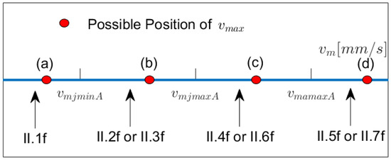
Figure 13.
Possible positions of and models for “going forth”.
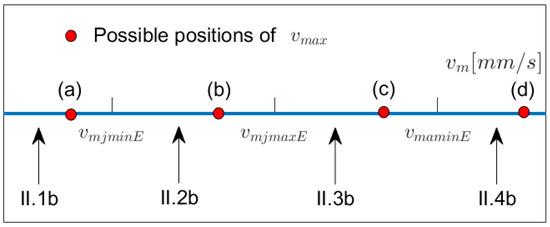
Figure 14.
Possible positions of and models for “going back”.
Finally, we determine the applicable model when we go from to . First, we consider the going forth situation. As in Case I, we have to identify the critical jerk values where a model switch takes place. Our procedure is similar to that conducted in Case I. We refer to Figure 13. If the position of is as marked as (a) there is no switch, i.e., the model is still II.1f. If we have position (b), we proceed as follows:
- In Model II.1f, set and , and compute by proceeding as stated in Algorithm A5, line 2, denoted by . There must be a solution, since we must end up with a symmetric model, and Model II.2f is not symmetric.
- For , apply Model II.2f; for , Model II.1f.
If situation (c) applies, the procedure is as follows:
- In Model II.4f, set and (i.e., the phase of constant maximal jerk has duration zero), and compute by proceeding as stated in Algorithm A5, line 5, denoted by in case of existence. If there is such a solution, the next model is II.2f. If not, Model II.4f is suitable for all jerk values.
- If Model II.2f is next, set in this model and , and compute by proceeding as stated in Algorithm A5, line 2, denoted by . This, then, must exist, since Model II.2f is not symmetric. The next model is II.1f. So, for , take Model II.4f; for , apply Model II.2f; and for , Model I.1f.
If situation (d) applies, perform the following:
- In Model II.5f, set and (i.e., the phase of constant maximal acceleration has duration zero). Compute by proceeding as stated in Algorithm A5, line 13, denoted by . If there is such a solution, the next model is II.4f. Otherwise, Model II.5f is suitable for all jerk values.
- If Model II.4f is next, set and in this model, and compute by proceeding as stated in Algorithm A5, line 5, denoted by , in case of existence. If there is such a solution with , the next model is II.2f. If not, apply Model II.5f for and Model II.4f for .
- If Model II.2f is next, set and in this model, and compute by proceeding as stated in Algorithm A5, line 2, denoted by . This, then, must exist, since II.2f is not symmetric. Now, for , apply Model II.5f; for , Model II.4f; for , Model II.2f; and for , Model II.1f.
Next, we consider the going back situation and refer to Figure 14. If we have situation (a), Model II.5b is suitable for all jerk values. Note that, in situation (b–d), we have , which makes the inequalities a bit more compact. If situation (b) applies, we proceed as follows:
- In Model II.6b, set and , and compute by proceeding as stated in Algorithm A6, line 2, denoted by . There must be a solution, since we must end up with a symmetric model, and Model II.6b is not symmetric.
- For , apply Model II.6b; for , Model II.5b.
If situation (c) applies, perform the following:
- In Model II.7b, set and (i.e., the phase of constant maximal jerk has duration zero). Compute by proceeding as stated in Algorithm A6, line 5, denoted by , in case of existence. If there is such a solution, the next model is II.6b. Otherwise, Model II.7b is suitable for all jerk values.
- If Model II.6b is next, set and , and compute by proceeding as stated in Algorithm A6, line 2, denoted by . This, then, must exist, since Model II.6b is not symmetric. The next model then is II.5b. For , apply Model II.7b; for , Model II.6b; and for , Model II.5b.
In situation (d), we can perform the procedure of situation (c):
- In Model II.8b, set and , and compute by proceeding as stated in Algorithm A6, line 13, denoted by . If this does not exist, Model II.8b is suitable for all jerk values.
- If it does exist, the next model is II.7b, and we proceed as in (c), obtaining a total of up to three critical jerk values.
The remarks concerning the situation given for Case I also apply to Case II.
5. Implementation and Validation
We assume that the following data are given:
- The kinematic restrictions .
- The initial and final velocities , where .
- The distance .
The main task now consists of finding the intermediate velocity and corresponding jerk , such that the covered distance equals where “flows” from via to and stays there for an arbitrary period of time. Algorithm 1 sketches how this task can be achieved. Briefly explained, the algorithm determines all critical velocities and computes for each of them the distance covered using the appropriate models. If the given distance is exceeded, one knows the interval of critical velocities (including or ) within which must lie. A simple bisection method can then be applied to obtain a guaranteed solution. If even exceeds the distance one obtains for , then the critical jerks are determined. These might be differently sequenced, e.g., if we have going forth and going back, the ordering might be or the other way around. For each possible ordering, and for each critical jerk from to 0, the covered distance is computed using the appropriate models. If the given distance is exceeded, one knows the interval of critical jerks (including 0 and ) within which must lie. Again, a simple bisection method can then be applied to obtain a guaranteed solution. If even exceeds the distance one obtains for as intermediate velocity and jerk, one takes the models to be applied for and inserts a segment with constant maximal velocity, such that .
| Algorithm 1. Main Algorithm. | |
| Input | |
| Output | |
| 1: | Determine the critical velocities using the algorithms/formulae presented in Appendix B |
| 2: | |
| 3: | according to Equation (1) and Table 1 |
| 4: | If Then |
| 5: | |
| 6: | Determine the going forth model according to Table 1 according to Table A1 resp. A3 |
| 7: | Else |
| 8: | For Each ) |
| 9: | |
| 10: | If Then |
| 11: | ) |
| 12: | Else |
| 13: | ) and the actual critical velocity. |
| 14: | Determine the models going forth and going back according to Figure 7 and Figure 8 resp. 13, 14. |
| 15: | according to Appendix A. |
| 16: | Return |
| 17: | End If |
| 18: | End For Each % End to line 8 |
| 19: | Determine the critical jerks using the algorithms presented in Appendix C |
| 20: | For Each possible sequence of critical jerks |
| 21: | For Each to 0 (including 0) |
| 22: | to |
| 23: | If Then |
| 24: | Pick next critical jerk (or 0) |
| 25: | Else |
| 26: | ) and the actual critical jerk, and the models to be applied are known according to the algorithms in Appendix C. |
| 27: | according to Appendix A. |
| 28: | Return |
| 29: | End If |
| 30: | End For Each % End to line 21 |
| 31: | End For Each % End to line 20 |
| 32: | must hold |
| 33: | according to Appendix A, . |
| 34: | End If % End to line 4 |
| 35: | Return |
We implemented the main algorithm and the auxiliary algorithms given in Appendix B and Appendix C as Matlab ® functions using the Matlab ® programming language. In these functions, the only calls to genuine mathematical facilities offered by Matlab ® are the ones to Matlab’s polynomial solver called “roots”. Therefore, when implementing the algorithms in another environment, only a polynomial solver needs to be programmed or imported from a mathematics library.
We set up the following test scenario in order to check whether viable results are provided:
- are chosen randomly between 5 and 100 (, , and , respectively; in the sequel, we will omit the units).
- is chosen randomly between and , between and .
- is chosen randomly between and .
We generated test configurations and checked and stopped the bisection iteration when the resulting distance was reached with a maximal error of (i.e., ). We also checked the error regarding and . In addition, we counted whether all possible combinations for positioning depicted in Figure 7 and Figure 8 for Case I and in Figure 13 and Figure 14 for Case II are covered, as well as all feasible combinations of numbers of values. Table 3 and Table 4 provide the values for Case I; Table 5 and Table 6 those for Case II. Those entries that are marked with a star are not feasible. We will demonstrate the reasoning behind this by giving two examples:
Table 3.
Coverage of situations in Case I.
Table 4.
Coverage of combinations of values for in Case I.
Table 5.
Coverage of situations in Case II.
Table 6.
Coverage of combinations of values for in Case II.
- Assume, in Case II, that we have two values when “going forth”, so we must have situation (c). Then, three values for going back are only possible when we have situation (d) for “going back”, but then, because of , we must also have situation (d) for “going forth”, which is a contradiction. Note that not all values in the upper triangle of Table 6 need to be zero: for example, we can have the combination 0–1 in case of situation (c) “going forth” and situation (b) “going back”.
The data presented in Table 3, Table 4, Table 5 and Table 6 demonstrate a satisfactorily coverage of all possible combinations of situations and numbers of values.
Table 7 shows the maximum error regarding distance, final velocity and final acceleration, as well as the mean and maximum number of iterations performed by the bisection method in Cases I and II. The maximum error regarding distance is due to our stopping criterion for the bisection method. All errors regarding the final velocity above were recorded. The number of occurrences was below 10, and the maximum value is given in the table. No errors for larger than were recorded. It is clear that the boundary set for the maximum admissible error in Δs has a considerable influence on the number of iterations performed by the bisection method, but one cannot relate the values directly, since the bisection is not performed for distance intervals but for velocity or jerk intervals.
Table 7.
Maximum error and number of iterations in Cases I and II.
All runs were completed successfully. In initial trials, occasionally, a run did not succeed because of numerical problems. The latter were removed by applying the following measures:
- If certain velocity values are very close to each other (i.e., ), they are set as equal, e.g., if , set ; if , set ; if , set .
- If in the bisection method, the middle of the considered interval coincides with a boundary because of rounding, bisection is stopped, and the middle is taken.
- If , models I.1f and II.1f are simplified by removing the fourth time interval, which must be zero.
- When finding and checking the zeros of polynomials, small imaginary parts are neglected, and inequalities and equations of solutions are checked using an admissible error margin.
To be suitable for online trajectory generation, it should be possible to complete the computation within one controller cycle. As in [4] (cf. the discussion presented there), we use 1ms as length of such a cycle. Time data were generated using the respective “tic” and “toc” facilities offered by Matlab®, which start and stop a timer and provide information on the time spent between the calls. Since the time needed by Matlab ® varies considerably when one makes several computations using the same data set, we apply the same approach as in [4]: for each random configuration, we make 1000 runs and take the minimum time. We randomly generated 100.000 configurations. The time data are given in Table 8 for Cases I and II; the underlying hardware consisted of a desktop PC running Windows 10 with a Xeon E5-1630v4 processor working at 3.7 GHz and 32GB RAM. Although the mean values and standard deviations suggest that, in general, a boundary of 1ms can be achieved, the maximum values show that, occasionally, computation might take longer. Using the profiling tool in Matlab©, one can see that finding the roots of polynomials takes about 50% of the overall computation time. In the bisection iterations, only polynomials of degree 4 occur. Whereas Matlab© implements a general polynomial solver, there are special ones for degree four that are very efficient, needing only 0.5 μs per run (cf. the discussion and references in [4]). Even for 50 bisection iterations in models I.1f and I.4f resp. II.1f and II.5f, with two polynomials per iteration, this would reduce the time needed considerably, such that completion within 1 ms can be achieved (see also the discussion on code optimization in [4]).
Table 8.
Computational effort in Cases I and II.
6. Numerical Comparison with Related Work
In this section, we compare our results with two approaches from the literature that also apply a fifteen-segment profile with piecewise constant snap and claim to provide a time-optimal solution. For the point-to-point motion (abbreviated as RR, “rest-to-rest”) with initial and final velocity equal to zero, we consider the algorithm by Biagiotti and Melchiorri [11], and for the constant-velocity-to-constant-velocity situation (abbreviated as GG) with arbitrary initial and final velocities and zero acceleration and jerk, we consider the algorithm by Fan et al. [28], who assume zero jerk at the intermediate velocity . Ezair et al. [34] make the same assumption and hence should provide identical results, but they explicitly recognize the sub-optimality.
The algorithm presented by Biagiotti/Melchiorri (“CheckConstraintsT1” in [11]) is based upon rectangular filter functions and has four time parameters in case of piecewise constant snap functions. It is strikingly simple and hence seems to contradict the complexity of the situation as presented in this contribution. We first compare the results of a configuration of Case I: . We let run from to , compute according to [11] and sum up to obtain the overall time . Then, we compute the time intervals as specified in this article and sum up to obtain the overall time for our approach. Figure 15a depicts the two quite similar curves, but the plot of the improvement of our approach compared to [11] in Figure 15b (in %) reveals that, over the whole range of distances, there is a reduction in time, which goes up to about 1%.
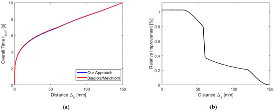
Figure 15.
(a) Overall time needed for going over the distance in [11] and in our approach. (b) Relative gain provided by our approach.
In order to better understand this difference, we picked one specific distance , with which we obtained the following results: the algorithm in [11] results in , summing up to ; our algorithm gives as models to be applied I.1f and I.1b with symmetric time interval lists. For model I.1f, we have , resulting in . We compare the jerk functions provided by both approaches in Figure 16. This shows that our approach takes full advantage of the lower jerk limit , whereas the algorithm of Biagiotti and Melchiorri [11] seems to enforce that the maximum and minimum value of the resulting jerk function have the same absolute value. This additional assumption might lead to a sub-optimal result. Actually, in the given configuration, we have Case I, so the maximum and minimum values of the resulting jerk function in our approach will have different absolute values over the full range of considered distances. Hence, our approach always results in a shorter time, as long as has not reached . This shows that the complexity of the situation demonstrated in this article cannot simply be sidestepped. Yet, it is fair to state that the approach by [11] can be extended to also include frequency restrictions, which makes it particularly interesting for vibration reduction.
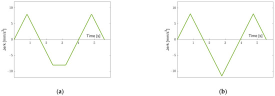
Figure 16.
(a) Jerk function provided by [11]. (b) Jerk function and in our approach.
The following configuration serves to compare our approach with the one by Fan et al. [28]: (Case I). Again, we let run from to and compute the overall time provided by our approach and by Fan et al., which is shown in Figure 17a. Here, the difference is well-recognizable. Figure 17b shows the relative improvement realized by our approach (in %), which goes up to 4.6%. If holds, we even found examples with a relative gain of up to 7%, which is due to the fact that the “base time” for going from directly to is zero. Numerical experiments also show that if is higher, the gain is reduced, since one can quickly get back from to zero.
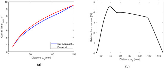
Figure 17.
(a) Overall time needed for going over the distance in [28] and in our approach. (b) Relative gain provided by our approach.
Again, it is fair to state that the algorithm by Ezair et al. [34] providing the same results as Fan et al. [28] has a wider range of applicability, since arbitrary boundary values for acceleration and jerk can also be prescribed, and it can be applied to higher orders.
7. Conclusions
In this contribution, we describe how a fast jerk–continuous motion function can be found when restrictions on velocity, acceleration, jerk and snap as well as initial and final values for velocity are given. We apply a fifteen-segment motion function with piecewise constant snap and ensure that, at each point in time, at least one restriction is reached, because of which we call the function fast. Note that, as shown in [4], this does not guarantee optimality. The research literature published so far has mainly dealt with point-to-point motions, where initial and final velocities are assumed to be zero, and the jerk becomes zero when the velocity takes its extremal value. We drop this assumption, which makes the situation much more complex, as was shown in the previous sections. Yet, the additional complexity is manageable by suitably structuring the problem in the following way:
- We distinguished two major cases depending on whether the maximum /minimum jerk value can be reached when going from acceleration zero to maximum/minimum acceleration.
- We picked an intermediate velocity with a corresponding jerk value and split up the motion in the velocity–acceleration plane into a going forth and a going back part.
- We identified all possible jerk models for going forth and back
- We identified the switching points for models by computing critical velocities and (at ) jerks.
By providing the corresponding algorithms, formulae and polynomials, a re-implementation is possible. Our own implementation in Matlab© showed that, in large test runs, a solution could always be found, and the complexity is necessary. Moreover, the investigation of time efficiency revealed that the computation should be achievable within a control cycle of 1 ms, where there is still considerable potential for improvement using dedicated quartic solvers.
We compared our approach with other motion functions suggested in the literature that apply the same fifteen-segment profile, since only those approaches allow us to stay at each restriction over a time interval of non-zero length. Numerical experiments revealed that a time improvement of up to 7% could be achieved compared to the algorithm by Fan et al., which also includes the case where initial and final velocities are non-zero. The algorithm by [11] is restricted to the point-to-point motion, and it is the only one that drops the additional assumption that the jerk must be zero when reaching the extremal velocity value. Yet, here, our algorithm showed an improvement of up to 1%, since the algorithm in [11] includes other assumptions, which, for certain configurations, make the algorithm sub-optimal.
The main progress compared to approaches that can be found in the literature can be summarized as follows:
- We take full advantage of restrictions on velocity, acceleration, jerk, and snap, and by dropping any additional assumption reducing optimality we provide the fastest currently available jerk-continuous motion function for rest-to-rest tasks and for tasks where initial and final velocities are given.
- In spite of the complexity caused by dropping any additional assumption our algorithm is still computationally efficient and hence suitable for Online Trajectory Generation.
Our improvement in time efficiency has its price, because it leads to a considerable extension of complexity. It certainly depends on the application whether the shorter processing time is worth this effort. Moreover, our approach has all the limitations that come with the application of fifteen-segment motion functions: the restrictions on jerk and snap are usually not provided in specifications of electronic drives but must be determined experimentally or taken from former experience. Another limitation of our approach consists of not taking into account the dynamics of manipulators, whereas in approaches working with optimization procedures, these can be easily included in the form of restrictions.
Given that the complexity our approach already has for the point-to-point and constant velocity-to-constant velocity task (termed RR and GG above), it might be worth investigating whether a general solution with arbitrary initial and final velocity, acceleration and jerk can be achieved. Further investigation is required to determine whether a reduction in the general case to the situation treated in this contribution is possible, as in [4].
Funding
The article processing charge was funded by the Baden-Württemberg Ministry of Science, Research and Culture and the Aalen University of Applied Sciences in the funding programme Open Access Publishing.
Institutional Review Board Statement
Not applicable.
Informed Consent Statement
Not applicable.
Data Availability Statement
Not applicable.
Conflicts of Interest
The authors declare no conflict of interest.
Appendix A. Formulae and Polynomials for Computing Time Intervals
Table A1.
Formulae and polynomials for computing time intervals in Case I going forth.
Table A1.
Formulae and polynomials for computing time intervals in Case I going forth.
| Model | Formulae and Polynomials | |
|---|---|---|
| I.1f | ||
| I.2f | ||
| I.3f | ||
| I.4f | ||
| I.5f | ||
| I.6f | ||
In all models holds.
Table A2.
Formulae and polynomials for computing time intervals in Case I going back.
Table A2.
Formulae and polynomials for computing time intervals in Case I going back.
| Model | Formulae and Polynomials | |
|---|---|---|
| I.1b | ||
| I.2b | ||
| I.3b | ||
| I.4b | ||
| I.5b | ||
| I.6b | ||
| I.7b | ||
Table A3.
Formulae and polynomials for computing time intervals in Case II going forth.
Table A3.
Formulae and polynomials for computing time intervals in Case II going forth.
| Model | Formulae and Polynomials | |
|---|---|---|
| II.1f | Same as Model I.1f | |
| II.2f | Same as Model I.2f | |
| II.3f | Same as Model I.5f | |
| II.4f | ||
| II.5f | ||
| II.6f | ||
| II.7f | ||
Table A4.
Formulae and polynomials for computing time intervals in Case II going back.
Table A4.
Formulae and polynomials for computing time intervals in Case II going back.
| Model | Formulae and Polynomials | |
|---|---|---|
| II.1b | Same as Model I.1b | |
| II.2b | Same as Model I.2b | |
| II.3b | ||
| II.4b | ||
| II.5b | Same as Model I.4b | |
| II.6b | Same as Model I.5b | |
| II.7b | ||
| II.8b | ||
Appendix B. Algorithms and Formulae for Computing Critical Velocities
| Algorithm A1. Algorithm for computing critical velocities in Case I going forth. | |
| Input: | |
| Output: | |
| 1: | If Then, % cf. Table 1 |
| 2: | |
| 3: | % for reaching |
| 4: | % according to Equation (6) |
| 5: | Return |
| 6: | End If |
| 7: | If |
| 8: | Find candidates for by determining the roots of the polynomial with coefficient vector (highest power first): |
| 9: | Pick for the real root with |
| 10: | Else set |
| 11: | End If |
| 12: | Determine in Model I.1f: |
| 13: | If Then, % jmin is reached first |
| 14: | % jm as determined in line 9 or 10. |
| 15: | |
| 16: | If Then, % is admissible |
| 17: | |
| 18: | Else % compute in Model I.5f |
| 19: | End If % from 16 |
| 20: | Else % amax is reached first |
| 21: | Find candidates for by determining the roots of the polynomial with coefficient vector (highest power first): |
| 22: | Pick for the real root with |
| 23: | |
| 24: | % for reaching |
| 25: | |
| 26: | End If % from line 13 |
| 27: | Return |
Table A5.
Formulae for computing critical velocities in Case I going back.
Table A5.
Formulae for computing critical velocities in Case I going back.
| Algorithm A2. Algorithm for computing critical velocities in Case II going forth. | |
| Input | |
| Output | |
| 1: | If Then % cf. Table 1 |
| 2: | |
| 3: | Then % cf. Table 1 |
| 4: | |
| 5: | Else % use first Model II.4f and, if not successful, try Model II6.f |
| 6: | |
| 7: | is admissible |
| 8: | |
| 9: | Else |
| 10: | |
| 11: | End If % line 7 |
| 12: | End If % line 3 |
| 13: | Else |
| 14: | If |
| 15: | by determining the roots of the polynomial with coefficient vector (highest power first); same as in Algorithm A1 line 8 |
| 16: | |
| 17: | Else |
| 18: | End If % line 14 |
| 19: | |
| 20: | in Model II2.f: |
| 21: | is admissible |
| 22: | |
| 23: | Else % Move to Model II.3f |
| 24: | |
| 25: | End If % line 7 |
| 26: | in Model II.4f |
| 27: | |
| 28: | is admissible |
| 29: | |
| 30: | Else % Model II.4f provides no solution, go to Model II.6f |
| 31: | |
| 32: | End If % line 28 |
| 33: | End If % line 1 |
| 34: | Return |
Table A6.
Formulae for computing critical velocities in Case II going back.
Table A6.
Formulae for computing critical velocities in Case II going back.
Appendix C. Polynomials and Formulae for Computing Critical Jerks
| Algorithm A3. Computing critical jerks and models in Case I “going forth”. | |
| Input:, situation % situation according to Figure 7 | |
| Output: (possibly empty) list of values (), list of models | |
| 1: | IfThen % for situation=a there is nothing to do, see Section 3 |
| 2: | Compute roots of and select the real negative with and . For the latter to be case, the following equation must hold: |
| 3: | and models=(I.2f,I.1f) |
| 4: | Else ifThen |
| 5: | . For the latter to be case, the following equation must hold: |
| 6: | resp. empty list and models=(I.3f,I.1f) resp. models=(I.3f) |
| 7: | Else ifThen |
| in the formula for in Model I.4f (Table A2) | |
| 8: | If Then |
| 9: | |
| 10: | next_model=I.3f |
| 11: | Else |
| 12: | Compute the roots of |
| 13: | taken from the previous line |
| 14: | next_model=I.2f |
| 15: | End If |
| 16: | If next_model=I.3f Then |
| 17: | if this exists (situation=c) |
| 18: | , models=(I.4f,I.3f,I.1f) resp. models=(I.4f,I.3f) |
| 19: | Else % next_model=I.2f |
| 20: | (situation=b) |
| 21: | , models==(I.4f,I.2f,I.1f) |
| 22: | End If |
| 23: | End If |
| 24: | Return |
| Algorithm A4. Computing critical jerks and models in Case I “going back”. | |
| Input, situation % situation according to Figure 8 | |
| Output), list of models | |
| 1: | If Then % for situation=a there is nothing to do, see Section 3 |
| 2: | . For the latter to be case, the following equation must hold: |
| 3: | and models=(I.5b,I.4b) |
| 4: | Else if Then |
| 5: | in the formula for in Model I.7b (Table A2) |
| 6: | If Then |
| 7: | |
| 8: | next_model=I.6b |
| 9: | Else |
| 10: | Compute the roots of . For the latter to be case, the following equation must hold: |
| 11: | |
| 12: | next_model=I.5b |
| 13: | End If |
| 14: | If next_model=I.6b Then |
| 15: | . For the latter to be case, the following equation must hold: |
| 16: | exists Then |
| 17: | and models=(I.7b,I.6b,I.4b) |
| 18: | Else |
| 19: | and models=(I.7b,I.6b) |
| 20: | End If |
| 21: | Else % next_model=I.5b |
| 22: | and models=(I.7b,I.5b,I.4b) |
| 23: | End If |
| 24: | End If |
| 25: | Return |
| Algorithm A5. Computing critical jerks and models in Case II “going forth”. | |
| Input: , situation % situation according to Figure 13 | |
| Output: (possibly empty) list of values (), list of models | |
| 1: | If Then % for situation=a there is nothing to do, see Section 4 |
| 2: | Compute roots of and select the real negative with and . For the latter to be case, the following equation must hold: % line 2 is identical to line 2 in Algorithm A3 |
| 3: | and models=(II.2f,II.1f) |
| 4: | Else if Then |
| 5: | Compute roots of and select the real negative root with , if existing. |
| 6: | If such a exists Then |
| 7: | |
| 8: | Proceed as in line 2, set and models=(II.4f,II.2f,II.1f) |
| 9: | Else |
| 10: | = empty list and models=(II.4f) |
| 11: | End If |
| 12: | Else if Then |
| 13: | Compute roots of and select the real negative root with , if existing. |
| 14: | If such a exists Then |
| 15: | |
| 16: | Proceed as in line 5 |
| 17: | If such a exists Then |
| 18: | |
| 19: | Proceed as in line 2, set , and models=(II.5f,II.4f,II.2f,II.1f) |
| 20: | Else |
| 21: | and Models = (II.5f, II.4f) |
| 22: | End If |
| 23: | Else |
| 24: | empty list, and models = (II.5f) |
| 25: | End If |
| 26: | End If |
| 27: | Return |
| Algorithm A6. Computing critical jerks and models in Case II “going back”. | |
| Input: , situation % situation according to Figure 14 | |
| Output: (possibly empty) list of values (), list of models | |
| 1: | If Then % for situation=a there is nothing to do, see Section 4 |
| 2: | Compute roots of and select the real negative with and . For the latter to be case, the following equation must hold: % line 2 is identical to line 2 in Algorithm A4 |
| 3: | and models=(II.6b,II.5b) |
| 4: | Else if Then |
| 5: | Compute roots of and select the real negative root with , if existing. |
| 6: | If such a exists Then |
| 7: | |
| 8: | Proceed as in line 2, set and models = (II.7b,II.6b,II.5b) |
| 9: | Else |
| 10: | empty list and models = (II.7b) |
| 11: | End If |
| 12: | Else if Then |
| 13: | Compute roots of and select the real negative root with , if existing. |
| 14: | If such a exists Then |
| 15: | |
| 16: | Proceed as in line 5 |
| 17: | If such a exists Then |
| 18: | |
| 19: | Proceed as in line 2, set , , and models=(II.8b,II.7b,II.6b,II.5b) |
| 20: | Else |
| 21: | ( and Models=(II.8b, II.7b) |
| 22: | End If |
| 23: | Else |
| 24: | empty list and models=(II.8b) |
| 25: | End If |
| 26: | End If |
| 27: | Return |
References
- Biagiotti, L.; Melchiorri, C. Trajectory Planning for Automatic Machines and Robots; Springer: Berlin/Heidelberg, Germany, 2008. [Google Scholar]
- Carbone, G.; Gomez-Bravo, F. (Eds.) Motion and Operation Planning of Robotic Systems; Mechanisms and Machine Science 29; Springer: Berlin/Heidelberg, Germany, 2015. [Google Scholar]
- Gasparetto, A.; Boscariol, P.; Lanzutti, A.; Vidoni, R. Path Planning and Trajectory Planning Algorithms: A General Overview. In Motion and Operation Planning of Robotic Systems; Carbone, G., Gomez-Bravo, F., Eds.; Springer: Berlin/Heidelberg, Germany, 2015; pp. 3–27. [Google Scholar]
- Alpers, B. On Fast Jerk-, Acceleration- and Velocity-Restricted Motion Functions for Online Trajectory Generation. Robotics 2021, 10, 25. [Google Scholar] [CrossRef]
- Sencer, B.; Altintas, Y.; Croft, E. Feed optimization for five axis CNC machine tools with drive constraints. Int. J. Mach. Tools Manuf. 2008, 48, 733–745. [Google Scholar] [CrossRef]
- Liu, H.; Lai, X.; Wu, W. Time-optimal and jerk-continuous trajectory planning for robot manipulators with kinematic constraints. Robot. Comput. Integr. Manuf. 2013, 29, 309–317. [Google Scholar] [CrossRef]
- Bharathi, A.; Dong, J. A Smooth Trajectory Generation Algorithm for Addressing Higher-Order Dynamic Constraints in Nanopositioning Systems. Proc. Manuf. 2015, 1, 216–225. [Google Scholar] [CrossRef] [Green Version]
- Fan, W.; Lee, C.; Chen, J. A realtime curvature-smooth interpolation scheme and motion planning for CNC machining of short line segments. Int. J. Mach. Tools Manuf. 2015, 96, 27–46. [Google Scholar] [CrossRef]
- Li, Y.; Huang, T.; Chetwynd, D.G. An approach for smooth trajectory planning of high-speed pick-and-place parallel robots using quintic B-splines. Mech. Mach. Theory 2018, 126, 479–490. [Google Scholar] [CrossRef] [Green Version]
- Da Rocha, P.A.S.; De Oliveira, W.D.; De Lima Tostes, M.E. An Embedded System-Based Snap Constrained Trajectory Planning Method for 3D Motion Systems. IEEE Access 2019, 7, 125188–125204. [Google Scholar] [CrossRef]
- Biagiotti, L.; Melchiorri, C. Trajectory generation via FIR filters: A procedure for time-optimization under kinematic and frequency constraints. Control Eng. Pract. 2019, 87, 43–58. [Google Scholar] [CrossRef]
- Fang, Y.; Qi, J.; Hu, J.; Wang, W.; Peng, Y. An approach for jerk-continuous trajectory generation of robotic manipulators with kinematical constraints. Mech. Mach. Theory 2020, 153, 103957. [Google Scholar] [CrossRef]
- Kröger, T.; Wahl, F.M. Online Trajectory Generation: Basic Concepts for Instantaneous Reactions to Unforseen Events. IEEE Trans. Robot. 2010, 26, 94–111. [Google Scholar] [CrossRef]
- Shiller, Z. Off-line and On-Line Trajectory Planning. In Motion and Operation Planning of Robotic Systems; Carbone, G., Gomez-Bravo, F., Eds.; Springer: Berlin/Heidelberg, Germany, 2015; pp. 29–62. [Google Scholar]
- Gasparetto, A.; Zanotto, V. A new method for smooth trajectory planning of robot manipulators. Mech. Mach. Theory 2007, 42, 455–471. [Google Scholar] [CrossRef]
- Zhang, Q.; Li, S. Efficient computation of smooth minimum time trajectory for CNC machining. Int. J. Adv. Manuf. Technol. 2013, 68, 683–692. [Google Scholar] [CrossRef]
- Fan, W.; Gao, X.; Lee, C.; Zhang, K.; Zhang, Q. Time-optimal interpolation for five axis CNC machining along parametric tool path based on linear programming. Int. J. Adv. Manuf. Technol. 2013, 69, 1373–1388. [Google Scholar] [CrossRef]
- Valente, A.; Baraldo, S.; Carpanzano, E. Smooth trajectory generation for industrial robots performing high precision assembly processes. CIRP Ann. Manuf. Technol. 2017, 66, 17–20. [Google Scholar] [CrossRef]
- Lin, J.; Somani, N.; Hu, B.; Rickert, M.; Knoll, A. An Efficient and Time-Optimal Trajectory Generation Approach for Waypoints under Kinematic Constraints and Error Bounds. In Proceedings of the IEEE/RSJ International Conference on Intelligent Robots and Systems (IROS), Madrid, Spain, 1–5 October 2018. [Google Scholar]
- Huang, J.; Hu, P.; Wu, K.; Zeng, M. Optimal time-jerk trajectory planning for industrial robots. Mech. Mach. Theory 2018, 121, 530–544. [Google Scholar] [CrossRef]
- Zhang, S.; Zanchettin, A.; Villa, R.; Dai, S. Real-time trajectory planning based on joint-decoupled optimization in human-robot interaction. Mech. Mach. Theory 2020, 144, 103664. [Google Scholar] [CrossRef]
- Ma, J.; Gao, S.; Yan, H.; Lv, Q.; Hu, G. A new approach to time-optimal trajectory planning with tork and jerk limits for robot. Robot. Auton. Syst. 2021, 140, 103744. [Google Scholar] [CrossRef]
- Biagiotti, L.; Melchiorri, C. Optimization of Generalized S-curve Trajectories for Residual Vibration Suppression and Compliance with Kinematic Bounds. IEEE/ASME Trans. Mechatron. 2021, 26, 2724–2734. [Google Scholar] [CrossRef]
- Wang, F.; Wu, Z.; Bao, T. Time-Jerk optimal Trajectory Planning of Industrial Robots Based on a Hybrid WOA-GA Algorithm. Processes 2022, 10, 1014. [Google Scholar] [CrossRef]
- Scalera, L.; Vidoni, R.; Giusti, A. Optimal scaling of dynamic safety zones for collaborative robotics. In Proceedings of the 2021 IEEE International Conference on Robotics and Automation (ICRA 2021), Xi’an, China, 31 May–4 June 2021; pp. 3822–3828. [Google Scholar]
- Lambrechts, P.; Boerlage, M.; Steinbuch, M. Trajectory planning and feedforward design for electromechanical motion systems. Contr. Eng. Pract. 2005, 13, 145–157. [Google Scholar] [CrossRef] [Green Version]
- Nguyen, K.D.; Ng, T.; Chen, I. On Algorithms for Planning S-curve Motion Profiles. Int. J. Adv. Robot. Syst. 2008, 3, 99–106. [Google Scholar] [CrossRef]
- Fan, W.; Gao, X.; Yan, W.; Yuan, C. Interpolation of parametric CNC machining path under confined jounce. Int. J. Adv. Manuf. Technol. 2012, 62, 719–739. [Google Scholar] [CrossRef]
- Lee, A.Y.; Choi, Y. Smooth trajectory planning methods using physical limits. J. Mech. Eng. Sci. 2015, 229, 2127–2143. [Google Scholar] [CrossRef]
- Fang, Y.; Hu, J.; Liu, W.; Shao, Q.; Qi, J.; Peng, Y. Smooth and time-optimal S-curve trajectory planning for automated robots and machines. Mech. Mach. Theory 2019, 137, 127–153. [Google Scholar] [CrossRef]
- Wang, H.; Wang, H.; Huang, J.; Zhao, B.; Quan, L. Smooth point-to-point trajectory planning for industrial robots with kinematical constraints based on high-order polynomial curve. Mech. Mach. Theory 2019, 139, 284–293. [Google Scholar] [CrossRef]
- Wu, Z.; Chen, J.; Bao, T.; Wang, J.; Zhang, L.; Xu, F. A Novel Point-to-Point Trajectory Planning Algorithm for Industrial Robots Based on a Locally Asymmetrical Jerk Motion Profile. Processes 2022, 10, 728. [Google Scholar] [CrossRef]
- Biagiotti, L.; Melchiorri, C.; Moriello, L. Damped Harmonic Smoother for Trajectory Planning and Vibration Suppression. IEEE Trans. Contr. Syst. Technol. 2020, 28, 626–634. [Google Scholar] [CrossRef]
- Ezair, B.; Tassa, T.; Shiller, Z. Planning high order trajectories with general initial and final conditions and asymmetric bounds. Int. J. Robot. Res. 2014, 33, 898–916. [Google Scholar] [CrossRef]
- Zhang, Y.; Ye, P.; Wu, J.; Zhang, H. An optimal curvature-smooth transition algorithm with axis jerk limitations along linear segments. Int. J. Adv. Manuf. Technol. 2018, 95, 875–888. [Google Scholar] [CrossRef]
- Zhang, L.; Du, J. Acceleration smoothing algorithm based on jounce limited for corner motion in high-speed machining. Int. J. Adv. Manuf. Technol. 2018, 95, 1487–1504. [Google Scholar] [CrossRef]
- VDI. Guideline 2143: Motion Rules for Cam Mechanisms: Theoretical Fundamentals; Beuth Verlag: Berlin, Germany, 1980. (In German) [Google Scholar]
- Broquère, X.; Sidobre, D.; Herrera-Aguilar, I. Soft motion trajectory planner for service manipulator robot. In Proceedings of the IEEE/RSJ International Conference on Intelligent Robots and Systems, Nice, France, 22–26 September 2008; pp. 2808–2813. [Google Scholar]
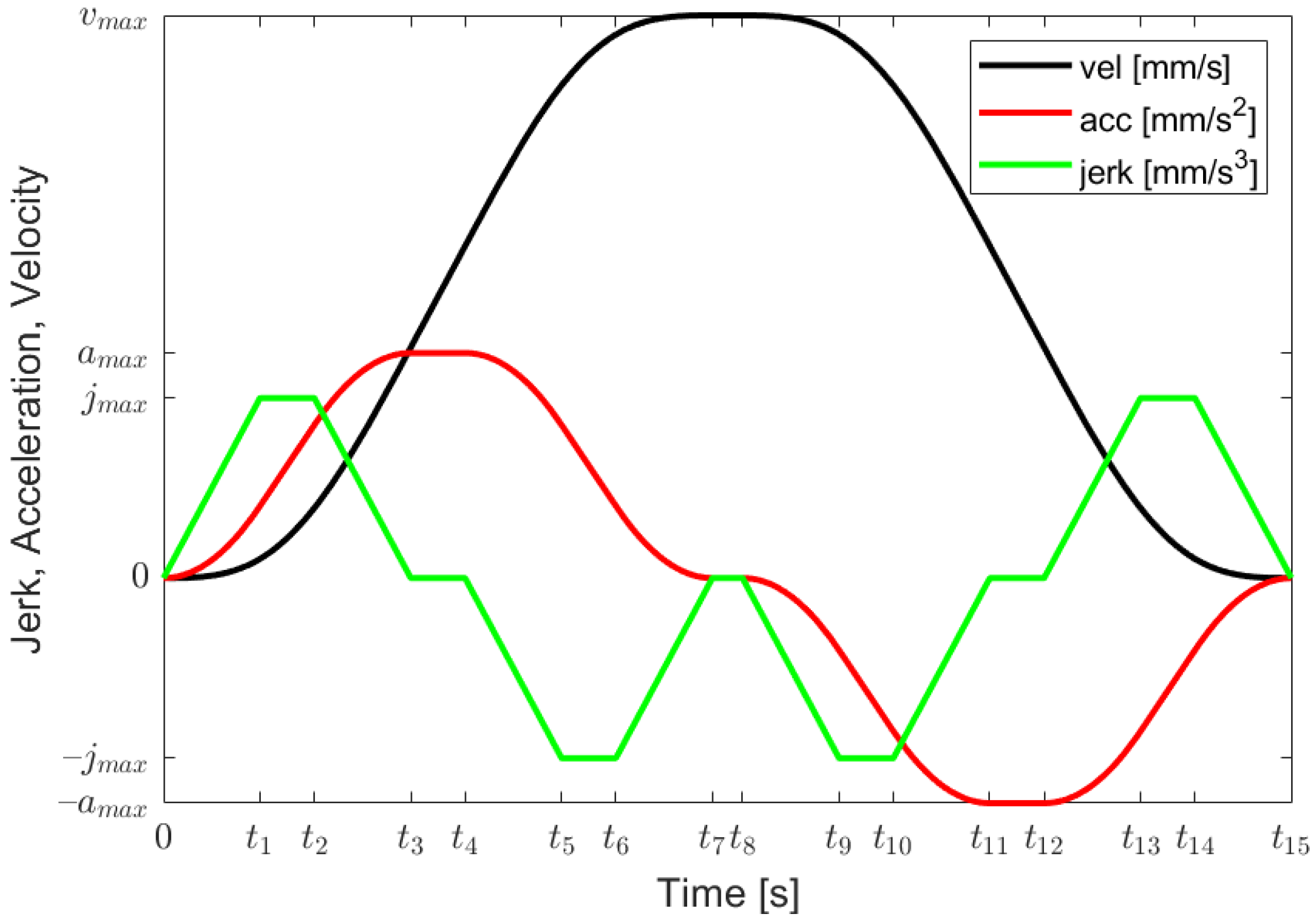
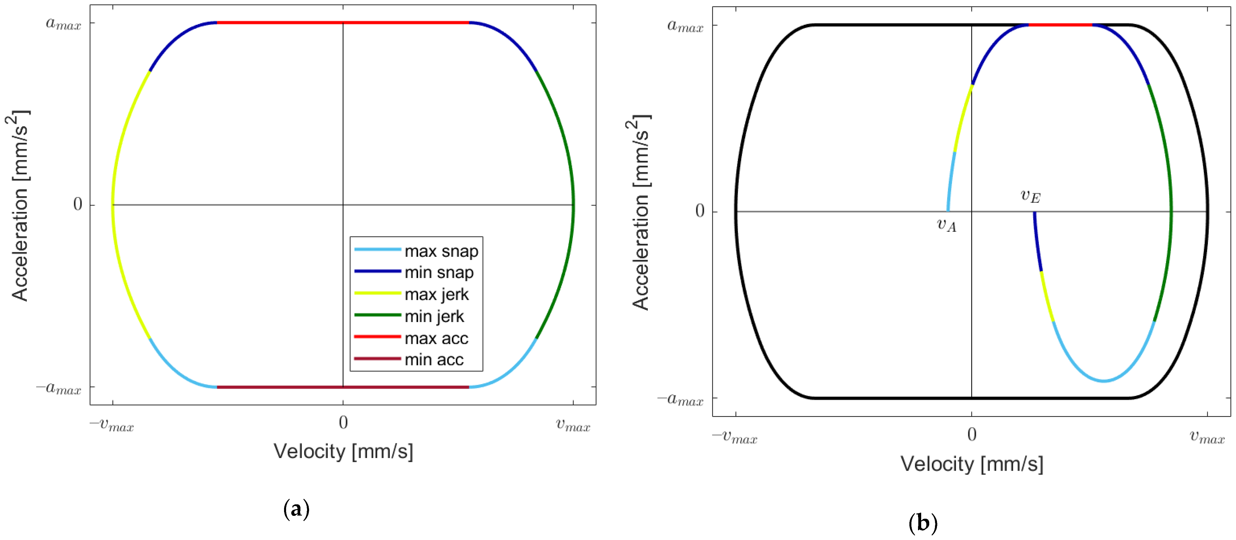

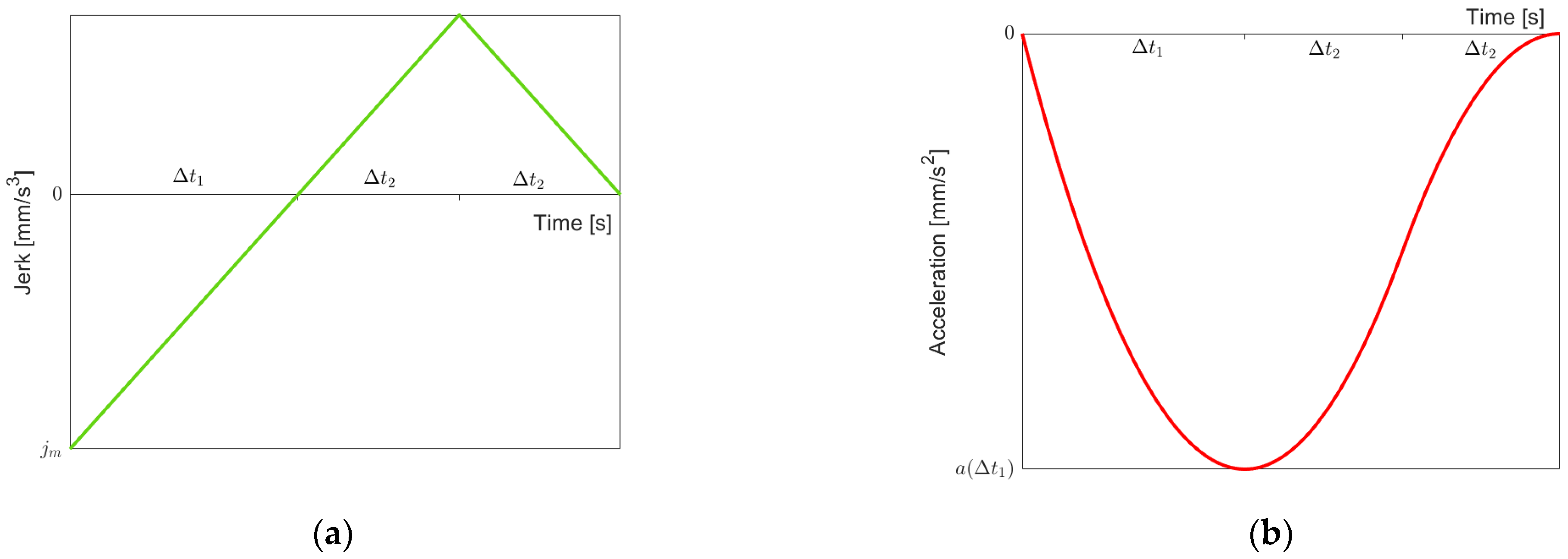
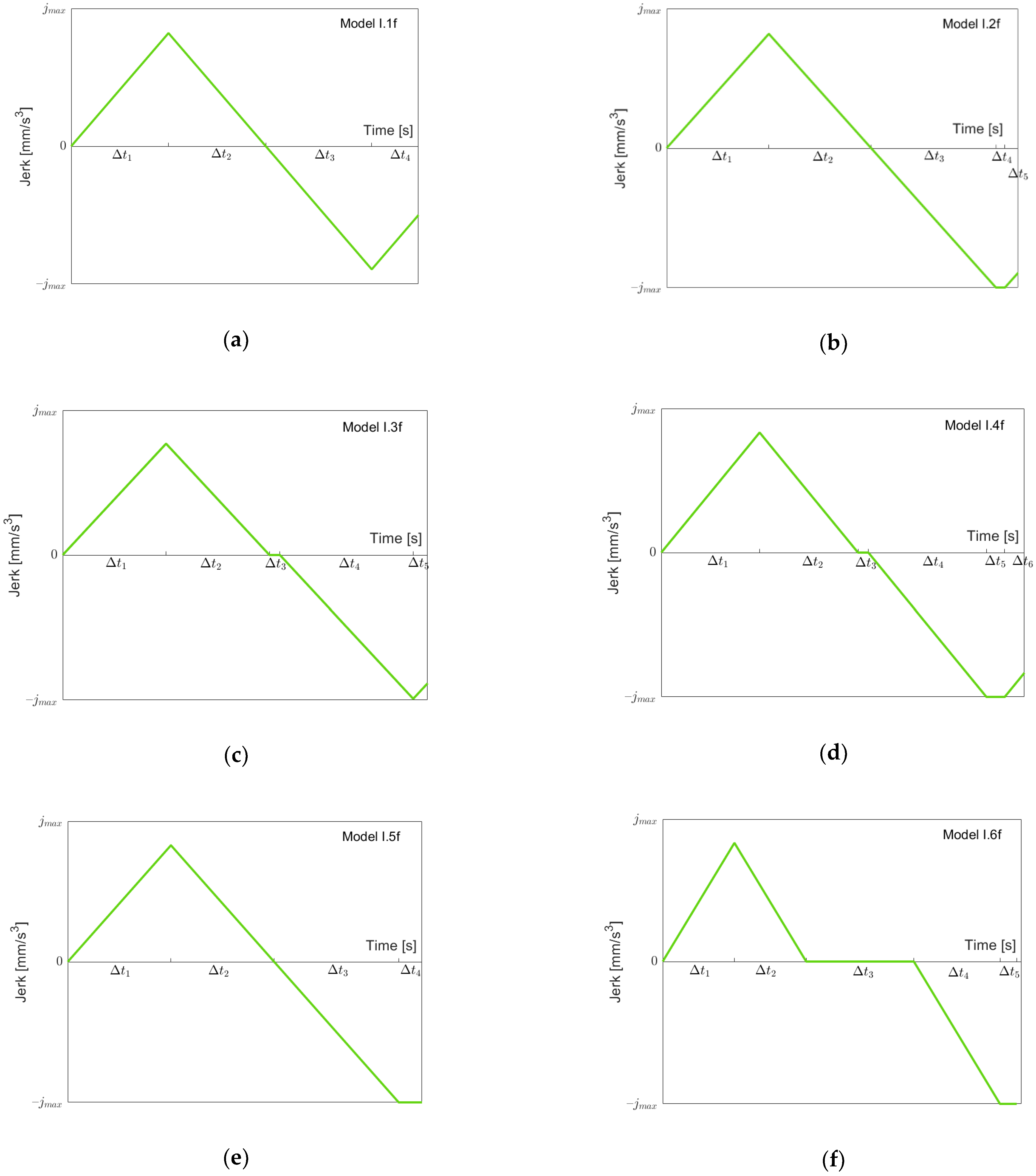
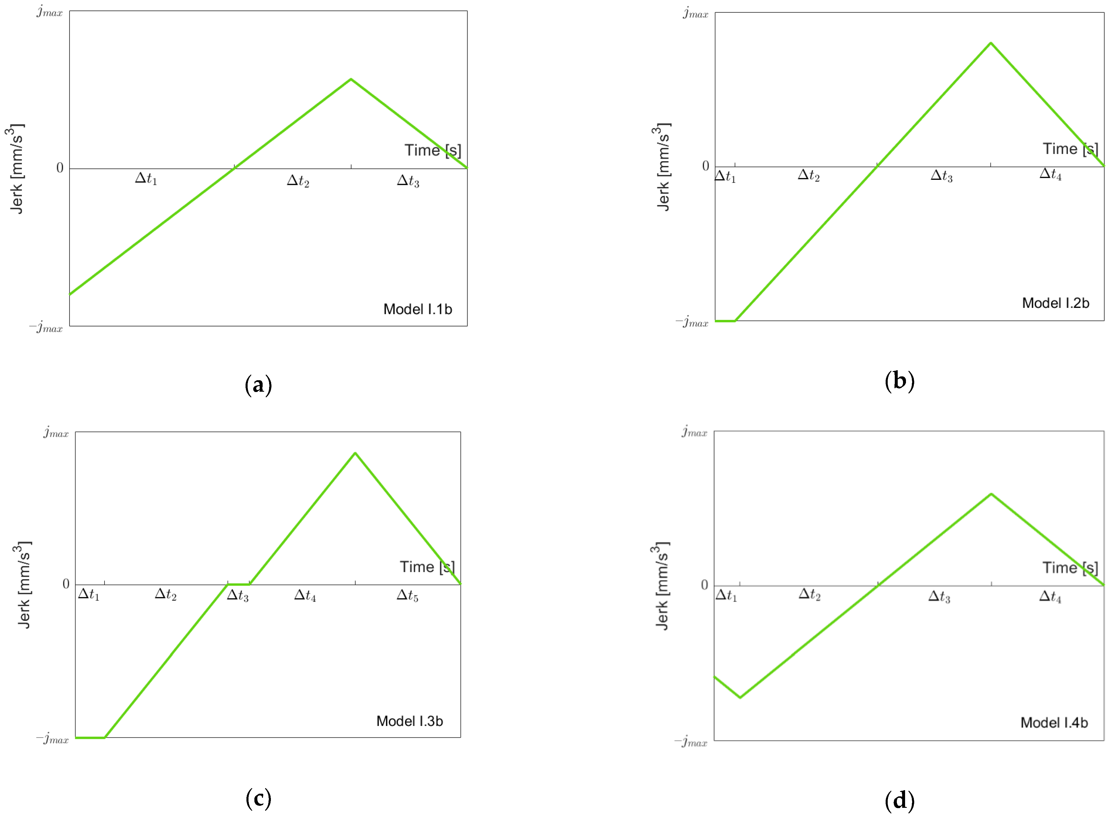
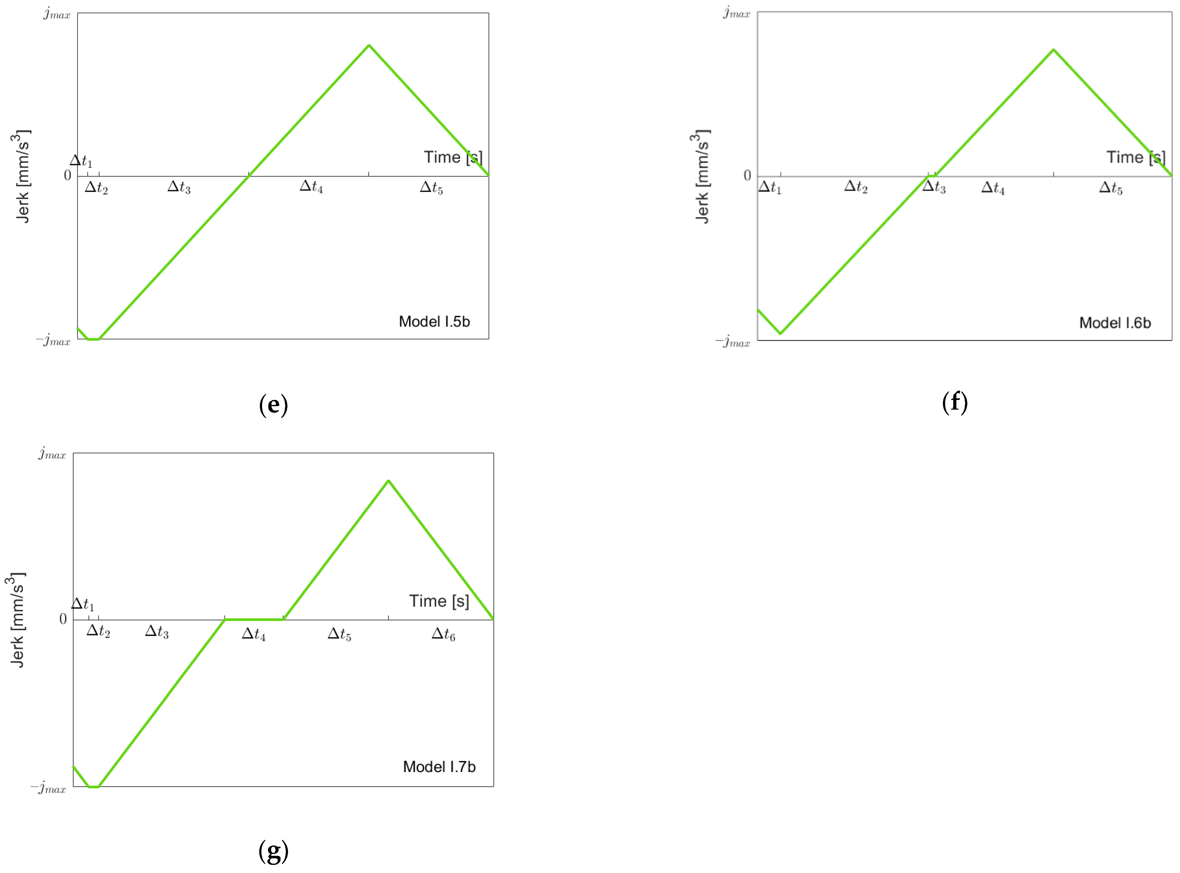

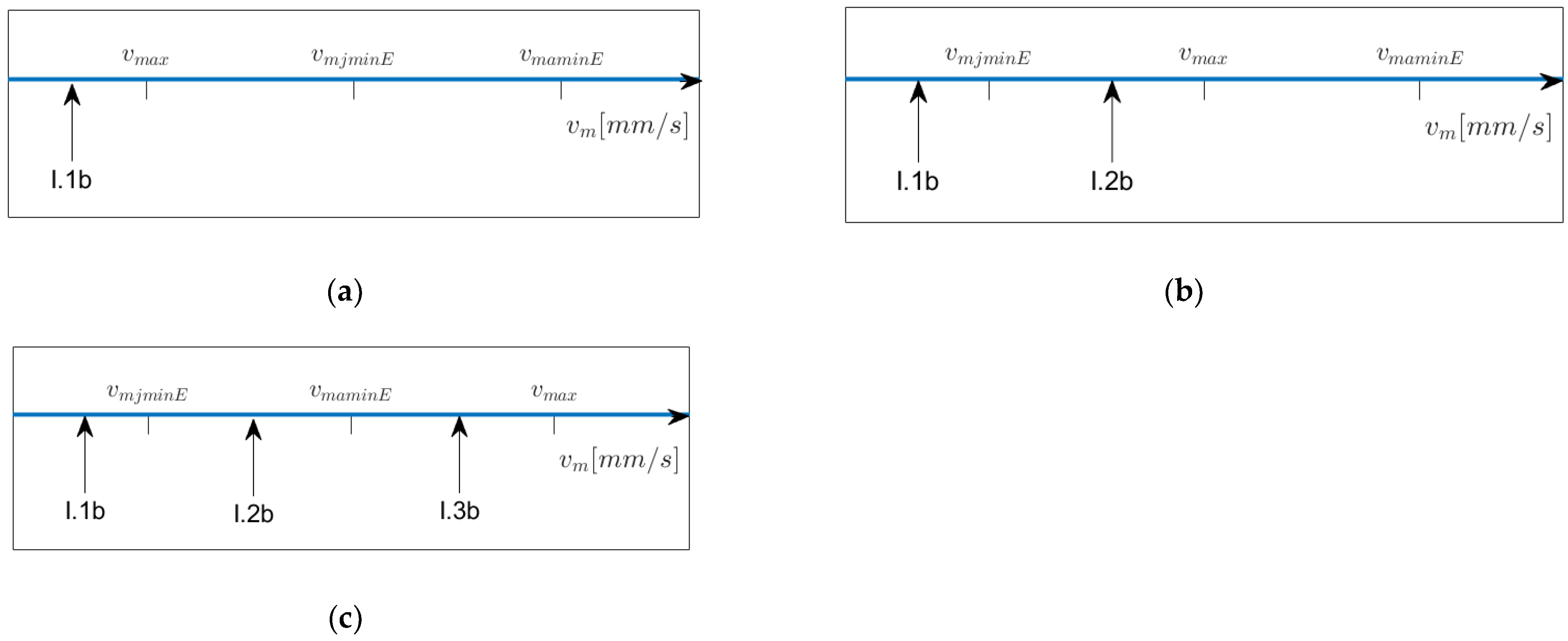
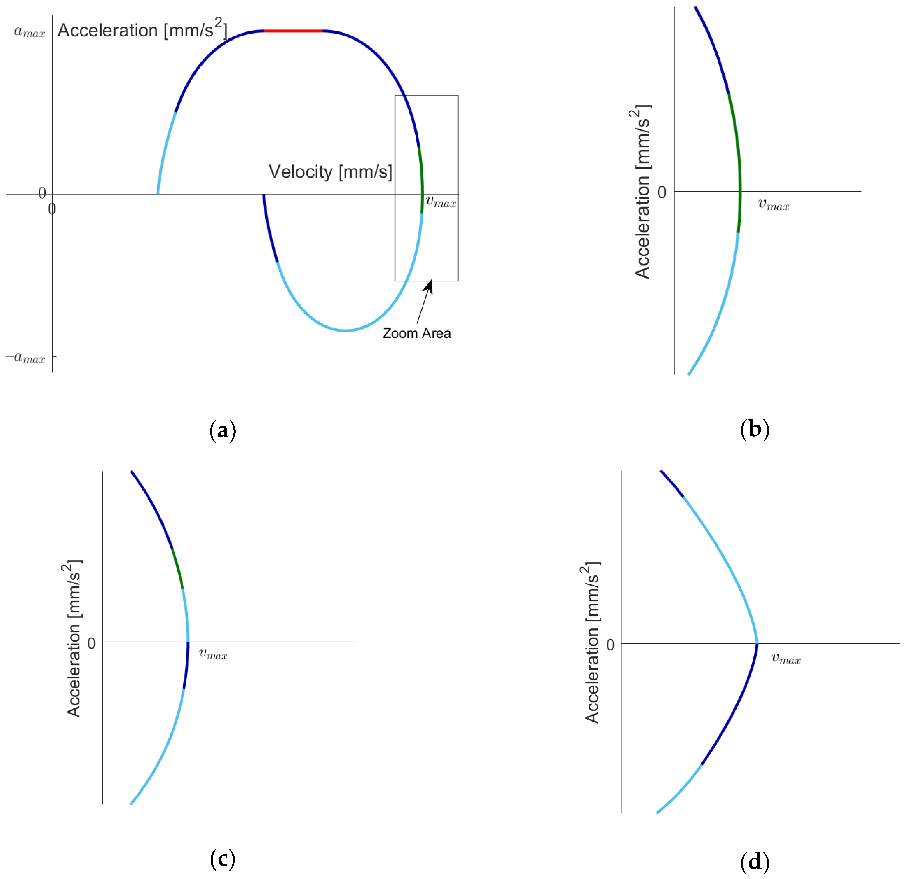
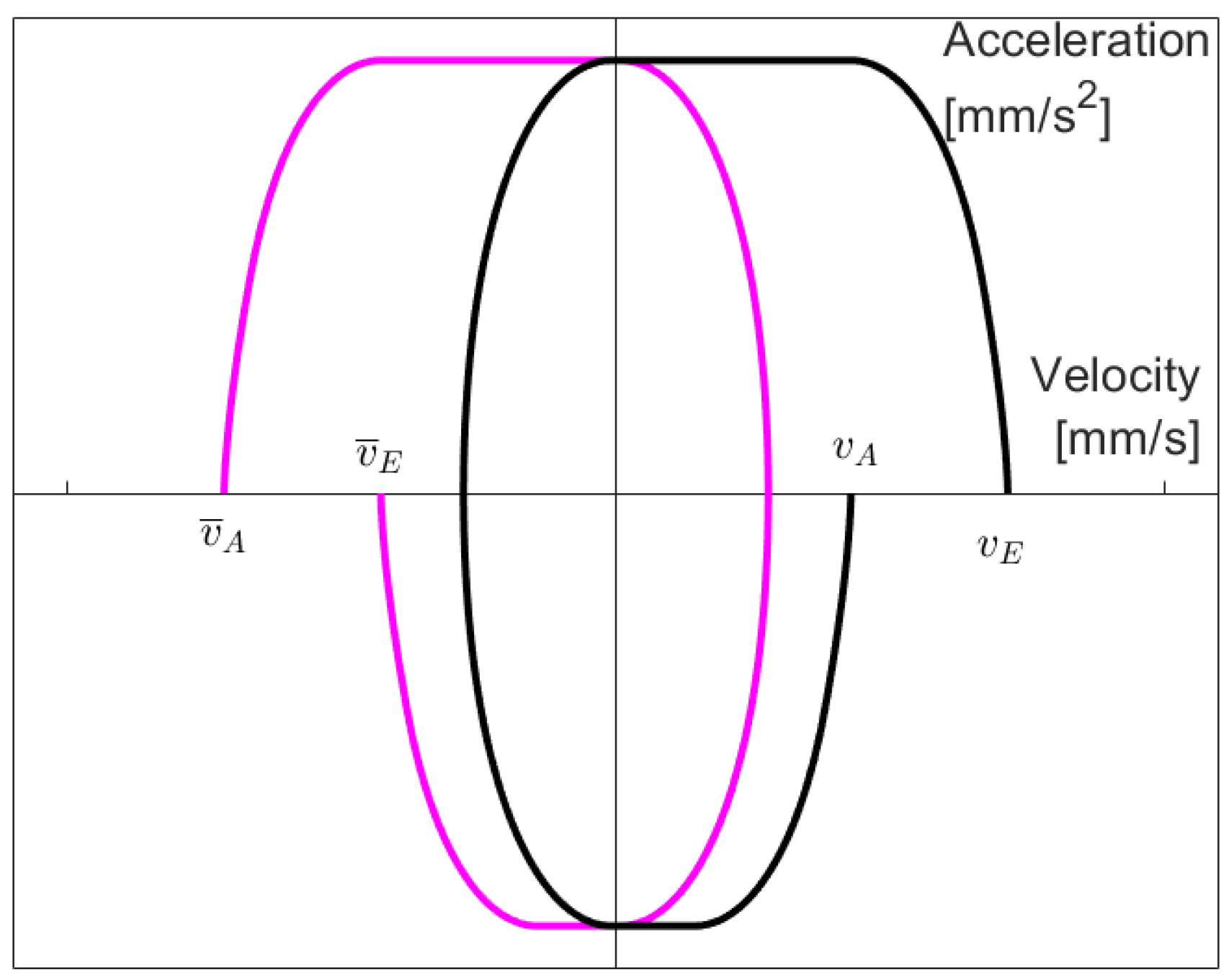
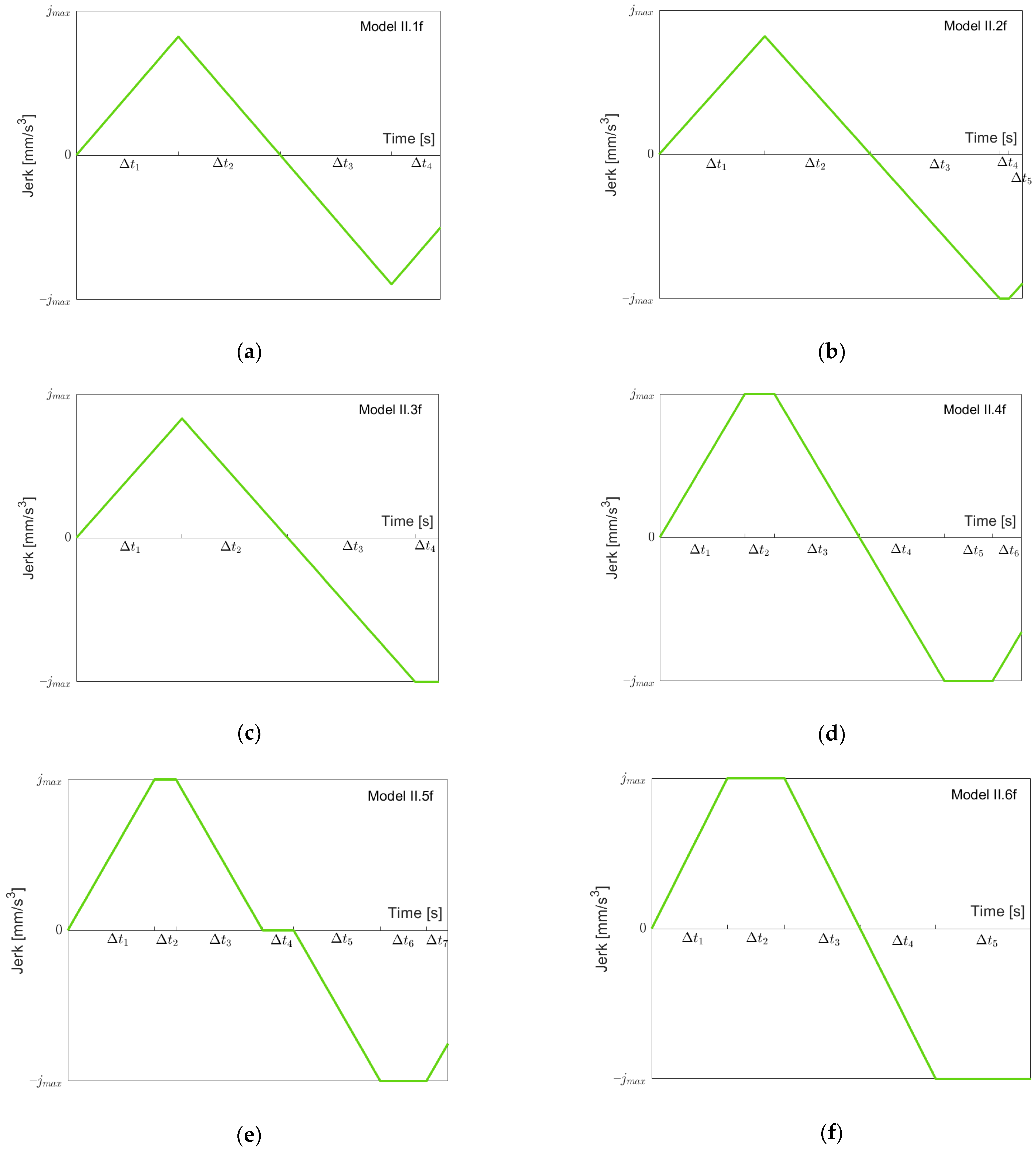
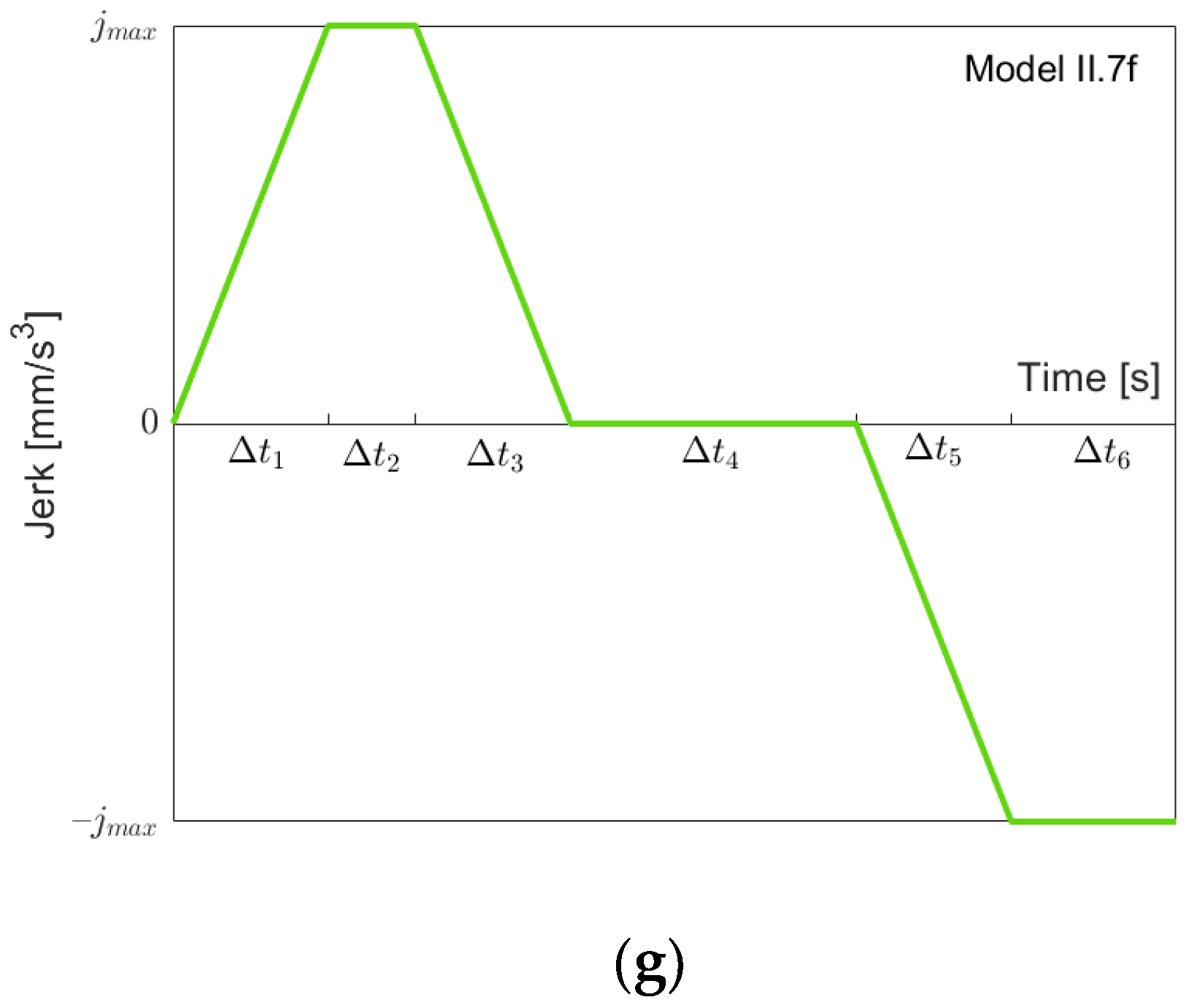
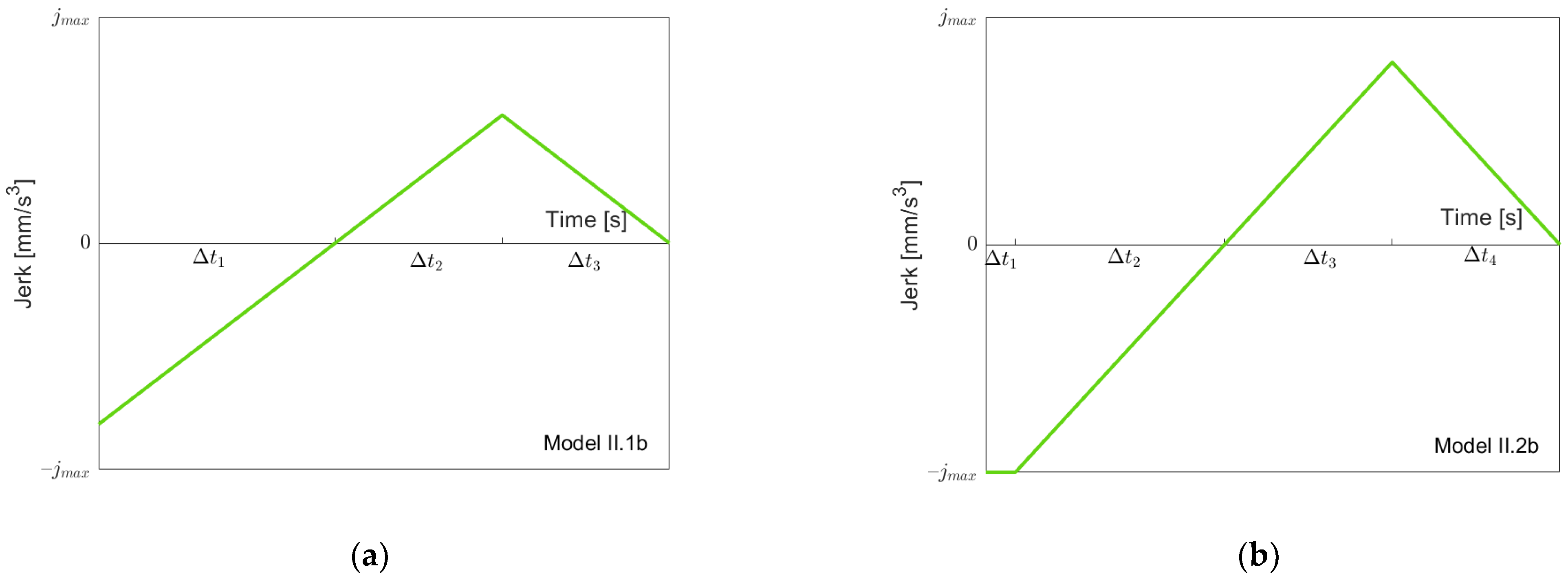
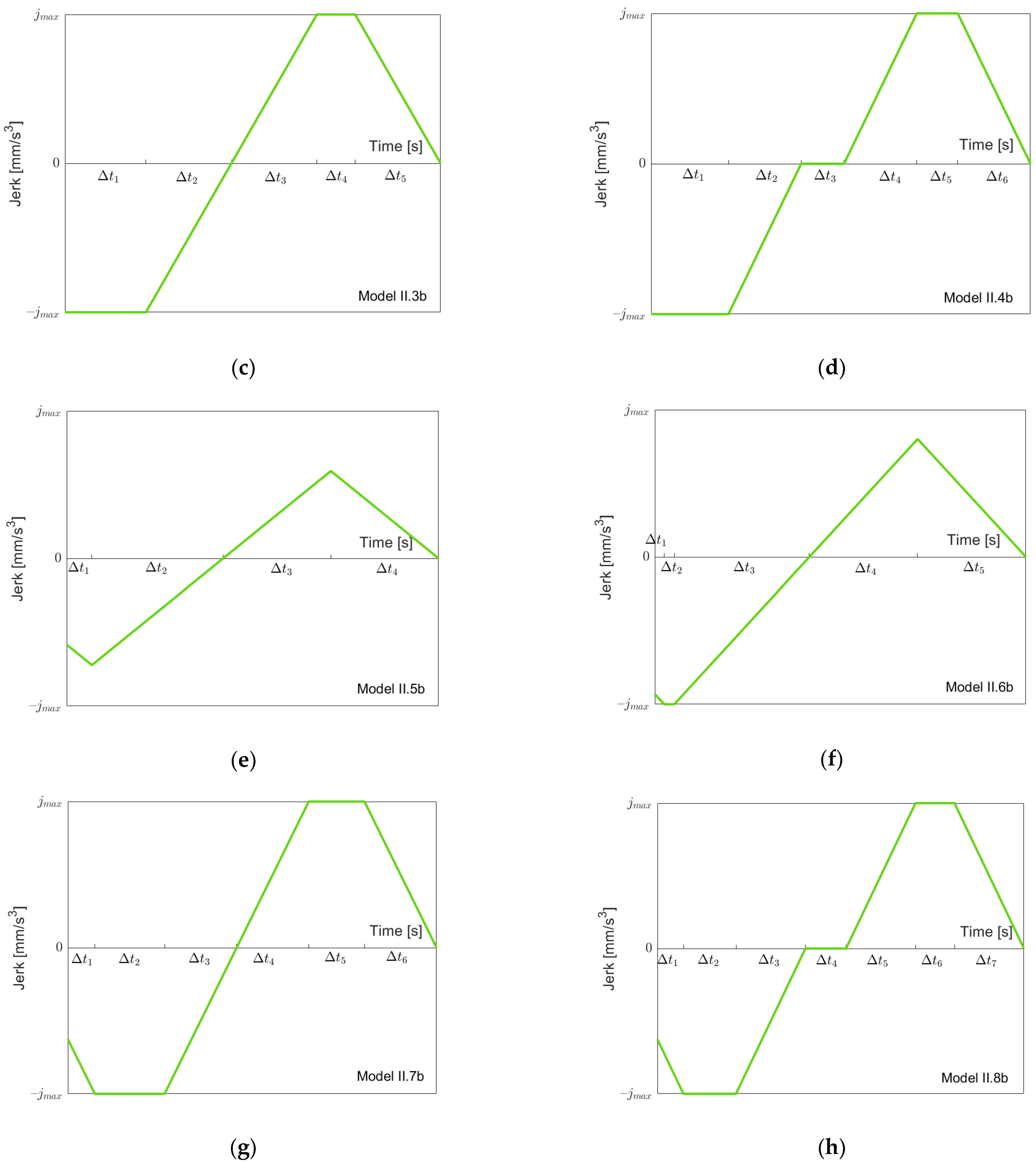
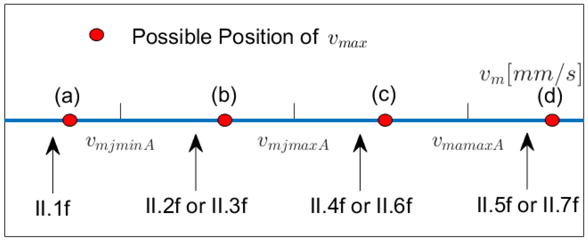
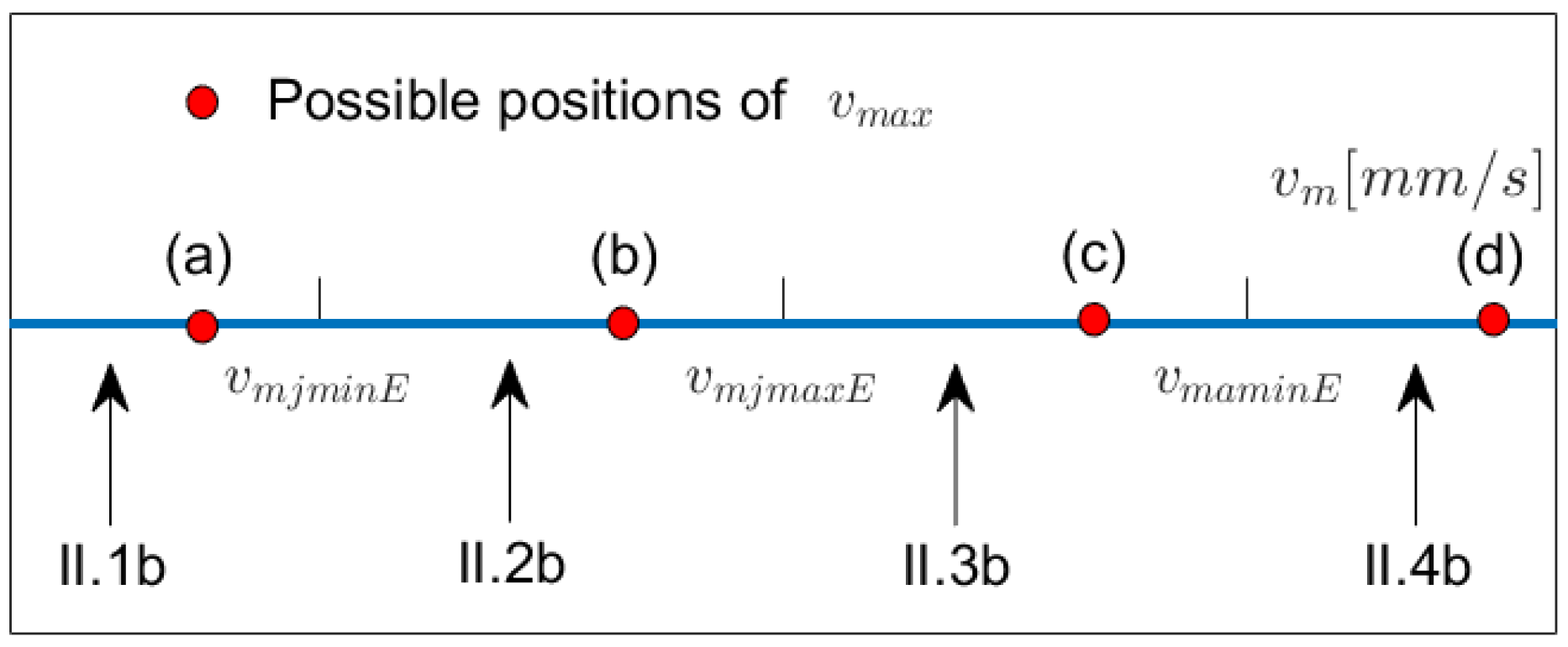
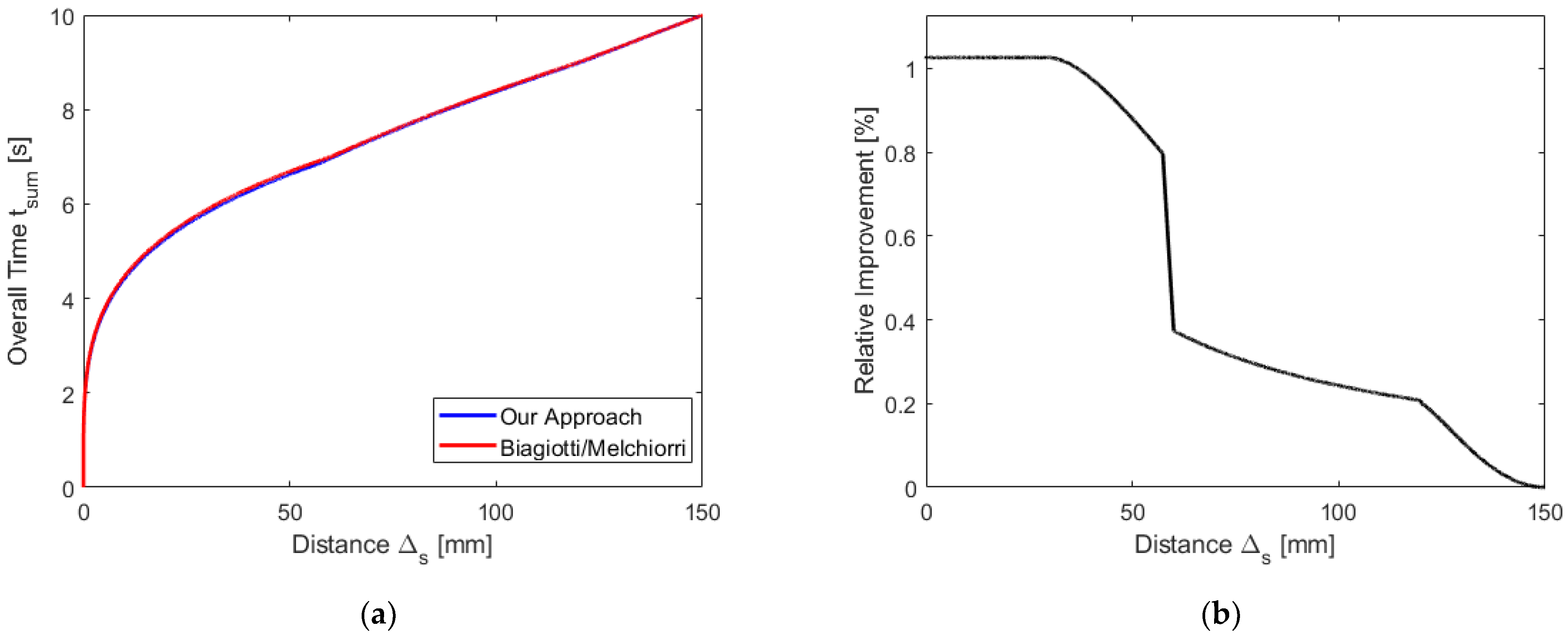
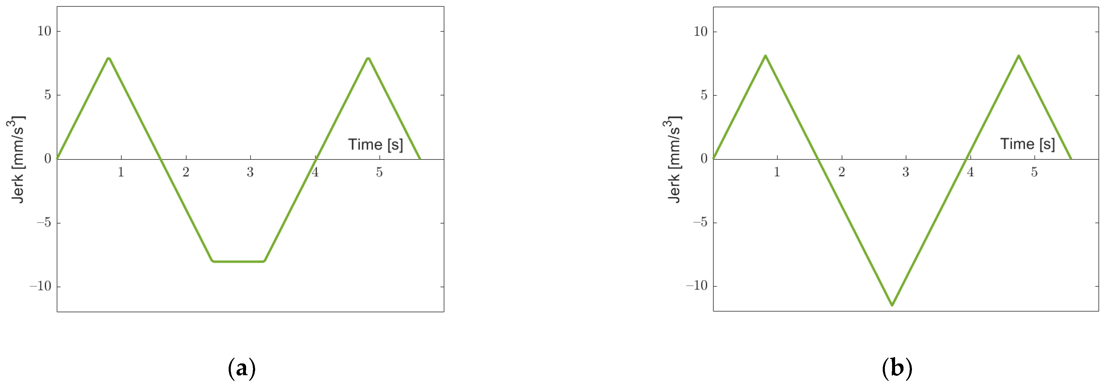

Publisher’s Note: MDPI stays neutral with regard to jurisdictional claims in published maps and institutional affiliations. |
© 2022 by the author. Licensee MDPI, Basel, Switzerland. This article is an open access article distributed under the terms and conditions of the Creative Commons Attribution (CC BY) license (https://creativecommons.org/licenses/by/4.0/).