1. Introduction
The tilt-rotor quadrotor [
1,
2,
3,
4], which is also referred to as the thrust vectoring quadrotor [
5,
6], is a novel type of quadrotor. Augmented with an additional mechanical structure [
7,
8], it is able to provide lateral force. Among the designs of the tilt-rotor, Ryll’s model, the tilt-rotor with eight inputs, received great attention in the last decade.
Various control methods have been analyzed in stabilizing Ryll’s model. These methods include feedback linearization [
1], geometric control [
9], PID (proportional integral derivative) control [
10], backstepping and sliding mode control [
11], etc. Among them, the feedback linearization is the first approach [
12] proposed in controlling Ryll’s model; this method decouples the original nonlinear system to generate the scenario compatible with the linear controller.
However, several unique properties of feedback linearization can hinder the application of this method. One of them is the saturation in feedback linearization [
13], which is parallel to the saturation in the geometric control [
14]. Also, the state drift phenomenon can be a problem [
15]. Another issue is the intensive change in the tilting angles while applying feedback linearization; the resulting changes in the tilting angles can be too large or too intensive. Notice that this intensive change in the tilting angles is not unique in the feedback linearization, e.g., PID [
16].
Generally [
17], the eight inputs are fully assigned by a united control rule, which makes the number of degrees of freedom less than [
12] or equal to [
10] the number of inputs. Indeed, these approaches avoid the under-actuated system. Further, the decoupling matrix in this scenario is invertible within the interested attitude region while applying feedback linearization. However, the adverse effect is the intensive change in the tilting angles mentioned beforehand, which may not be desired in application.
Our previous research [
18] averts this problem by decreasing the number of inputs of the tilt-rotor. Instead of assigning the tilting angles by the united control rule, a gait plan is applied to the tilting angles beforehand, leaving the magnitudes of thrusts the only actual control inputs. It produces an under-actuated control scenario with the attitude region introducing the singularity in the decoupling matrix. The tilting angles mimicked the cat-trot gait in other research [
19] about the tracking problems.
The cat-trot-inspired gait plan for the tilt-rotor guarantees that the decoupling matrix is always invertible during the entire flight, given that the attitude is close to zero, e.g., roll angle and pitch angle are close to zero [
19]. The determinant of the relevant decoupling matrix is proved non-zero analytically, assuming that the roll angle and pitch angle are zero.
Unfortunately, the determinant of the decoupling matrix of the gaits analyzed in this paper are not guaranteed to be non-zero without the restrictions on the attitude.
This paper provides novel gaits inspired by the rest of the typical cat gaits, both symmetrical (walk and run) and asymmetrical (transverse gallop and rotary gallop) [
20], for the tilt-rotor. The singularity of the decoupling matrix for each of these gaits is analyzed numerically; some gaits are modified by scaling to receive an invertible decoupling matrix before applying feedback linearization. Note that this scaling method is proved to be an effective approach to modify the unqualified gaits, e.g., the gait introducing invertible decoupling matrix only in a small region of the attitude, for a tilt-rotor for the first time.
The degrees of freedom tracked directly are attitude and altitude, e.g., roll, pitch, yaw, and altitude. The rest positions are influenced by manipulating the attitude properly; the modified position-attitude decoupler for the tilt-rotor advanced in the previous research [
19] is adopted to track the position.
Two references (uniform rectilinear motion and uniform circular motion) are designed for the tilt-rotor to track in the experiments. Each of the four gaits is applied and analyzed with different periods in the tracking experiment. The result of the position-tracking problem is also compared in the cases with or without advancing the attitude-altitude decoupler. The experiment is simulated in Simulink, MATLAB.
The rest of this paper is structured as follows.
Section 2 introduces the dynamics of the tilt-rotor. The controller and the gaits are designed in
Section 3.
Section 4 analyzes the singularity of the decoupling matrix in each gait and puts forward a gait modification method.
Section 5 sets up the references in the tracking problem. The result is demonstrated in
Section 6. The conclusions and discussions are addressed in
Section 7.
2. Dynamics of the Tilt-Rotor
This section details the dynamics of the tilt-rotor. A comprehensive discussion on it can be referred to in previous studies adopting the same dynamics model [
12,
18,
19].
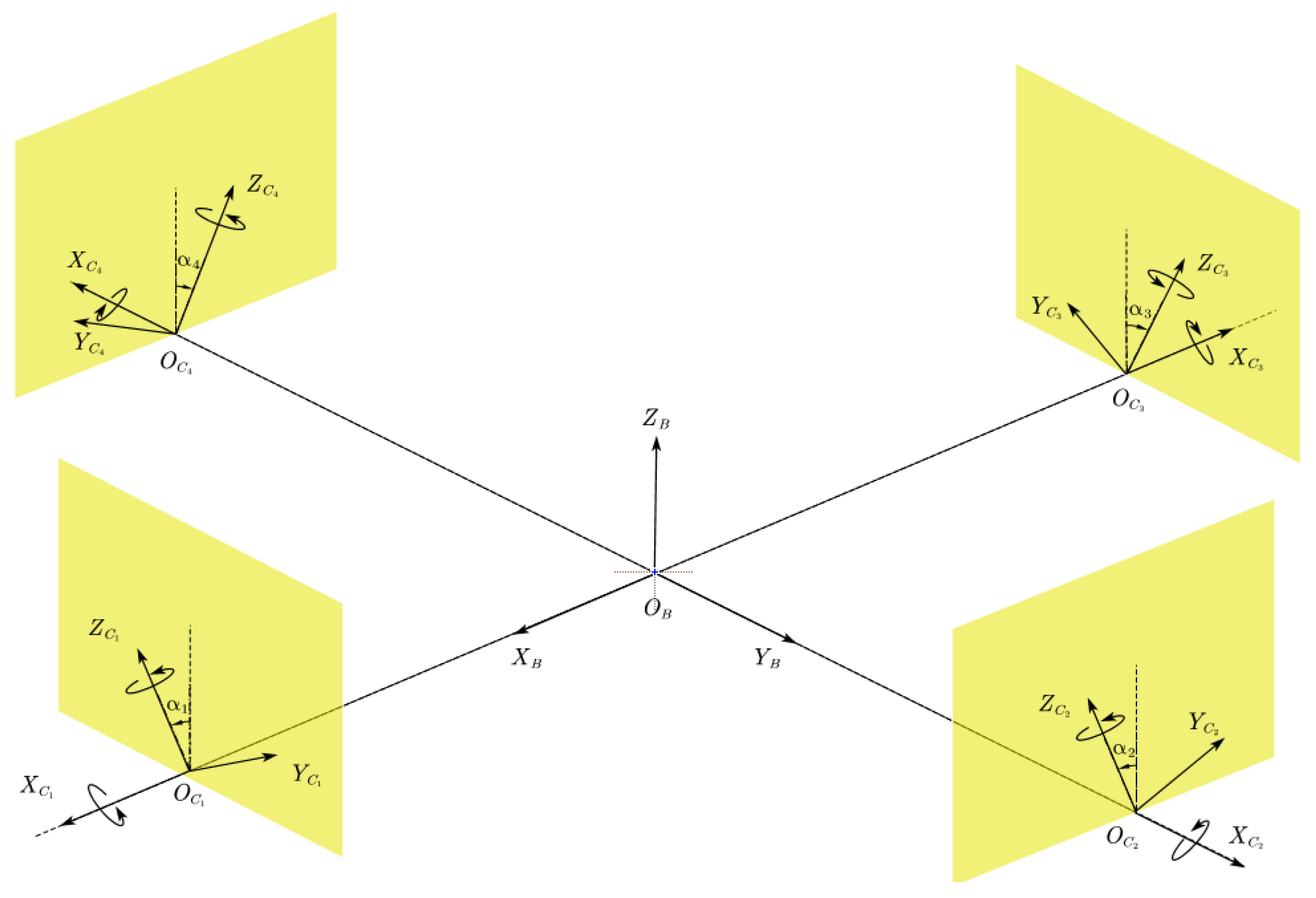
The model of the tilt-rotor investigated in this study,
Figure 1 [
18], was initially put forward by Ryll [
12].
The frames introduced in the dynamics of this tilt-rotor are the earth frame , body-fixed frame , and four rotor frames , each of which is fixed on the tilt motor mounted on the end of each arm. Rotor 1 and 3 are assumed to rotate clockwise along and . Rotor 2 and 4 are assumed to rotate counter-clockwise along and .
Based on the Newton-Euler formula, the position of the tilt-rotor [
18] is given by
where
represents the position with respect to
,
represents the total mass,
represents the gravitational acceleration,
, (
) represents the angular velocity of the propeller (
,
) with respect to
,
represents the rotational matrix [
21],
where
and
.
,
, and
are roll angle, pitch angle, and yaw angle, respectively, the tilting angles
. The positive directions of the tilting angles are defined in
Figure 1.
is given by
where
,
, and (
).
(
) is the coefficient of the thrust.
The angular velocity of the body with respect to
,
, is governed (Newton-Euler formula) by
where
is the matrix of moments of inertia,
(
) is the coefficient of the drag, and
is the length of the arm,
The relationship [
22,
23,
24] between the angular velocity of the body,
, and the attitude rotation matrix (
) is given by
where “
” is the hat operation used to produce the skew matrix,
represents the derivative of rotation matrix.
The parameters of this tilt-rotor are specified as follows: , , , .
3. Controller Design and Gait Plan
The same control method as in our previous research [
18,
19] is adopted. This section briefs this controller and introduces animal-inspired gaits analyzed in this study.
3.1. Feedback Linearization and Modified Attitude-Position Decoupler
The degrees of freedom controlled independently in this research are selected as attitude (, , and ) and altitude (Z).
Assuming
we receive
where
is called the decoupling matrix [
25],
is the new input vector, and
are the remaining terms not containing
,
,
, or
, which is
.
Finally, design the PD (proportional derivative) controller based on
where
represents the PD controller, which is detailed in
Appendix A.
Our previous research [
18] approximates the necessary and sufficient condition to receive an invertible decoupling matrix, given non-zero angular velocities in the propellers. That is
Once the gait (combination of the tilting angles) satisfies (11), the decoupling matrix in feedback linearization is asserted to be invertible in our case, given .
The next question is how to control the remaining degrees of freedom, and in position.
The conventional quadrotor tracks the position by adjusting its attitude based on the conventional attitude-position decoupler [
16,
24,
26]. This decoupler, however, may not be valid for a tilt-rotor. Our previous research [
19] deduced the modified attitude-position decoupler for the tilt-rotor,
where
and
are defined by
One of the comparisons we will make in the tracking result is the simulations equipped with the conventional attitude-position decoupler and with the modified attitude-position decoupler.
3.2. Symmetrical and Asymmetrical Cat-Inspired Gait
The gait for a tilt-rotor is defined as the combination of time-specified tilting angles. Our previous research [
19] deployed the cat-trot inspired gait, which leads to the invertible decoupling matrix, satisfying (11).
In this research, several other common cat gaits are discussed before being modified to accommodate (11) and being applied to the tilt-rotor-gait plan.
The cat gaits can be classified as symmetrical gaits and asymmetrical gaits. The footfalls in the former gaits touches the ground at evenly spaced interval of time, which is not the case for the latter gaits [
20]. Typical symmetrical gaits include walk, run, and trot. While transverse gallop and rotary gallop are asymmetrical gaits. The target gaits within the scope of this research are walk, run, transverse gallop, and rotary gallop.
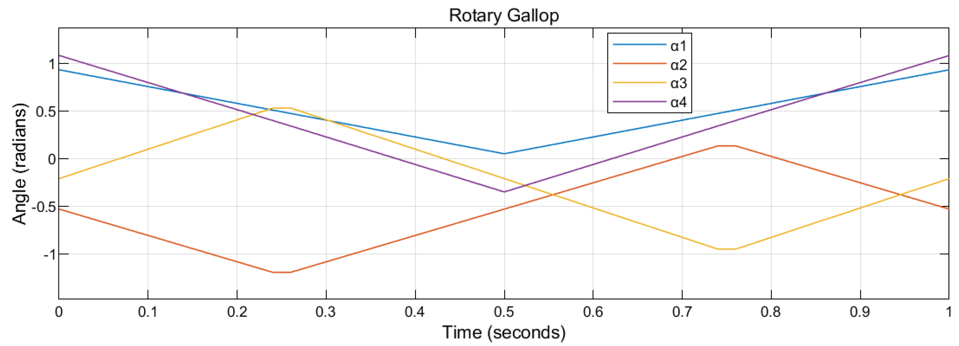
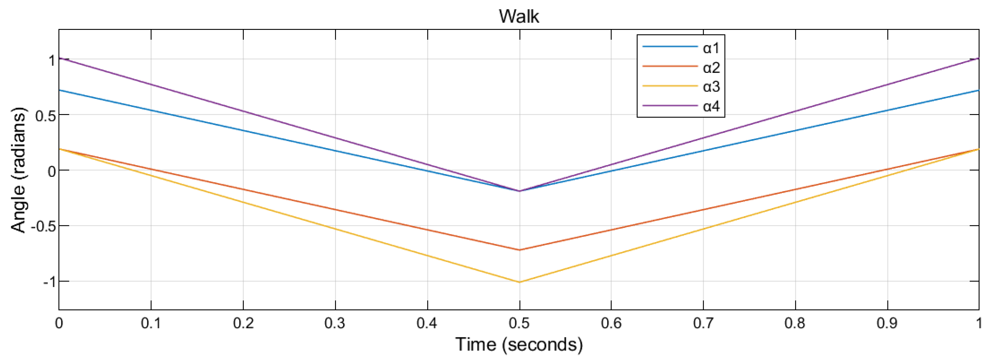
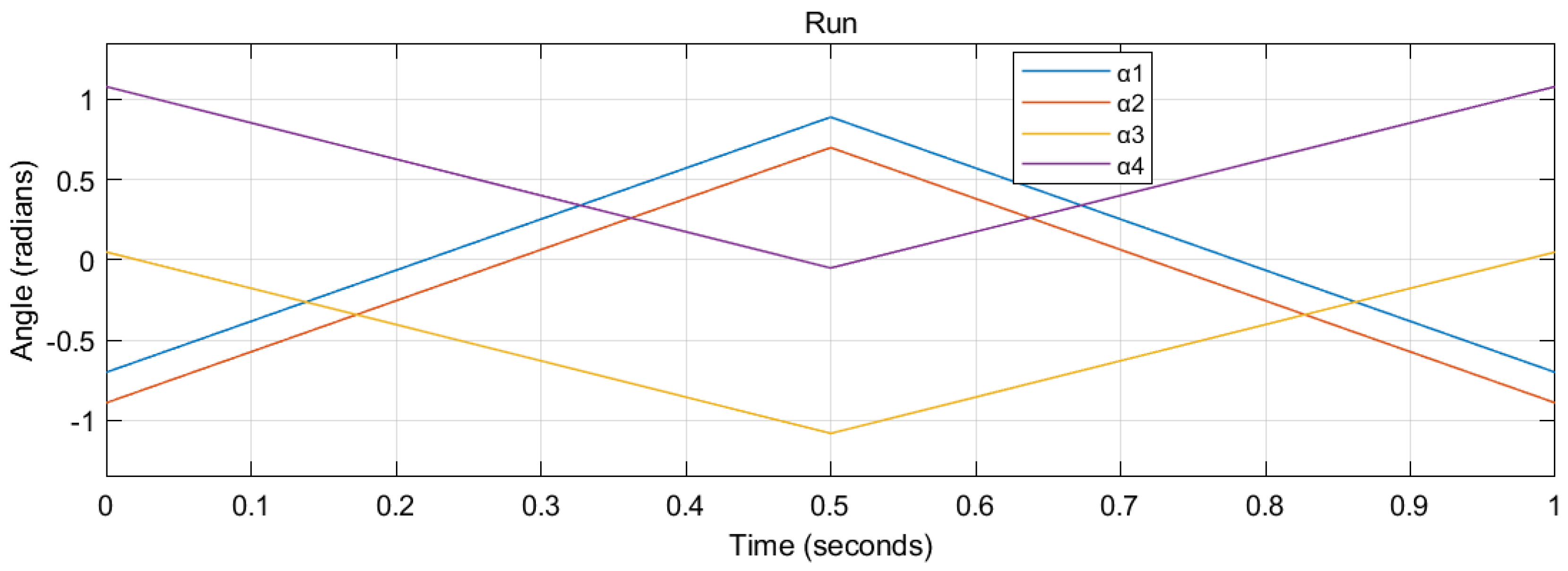
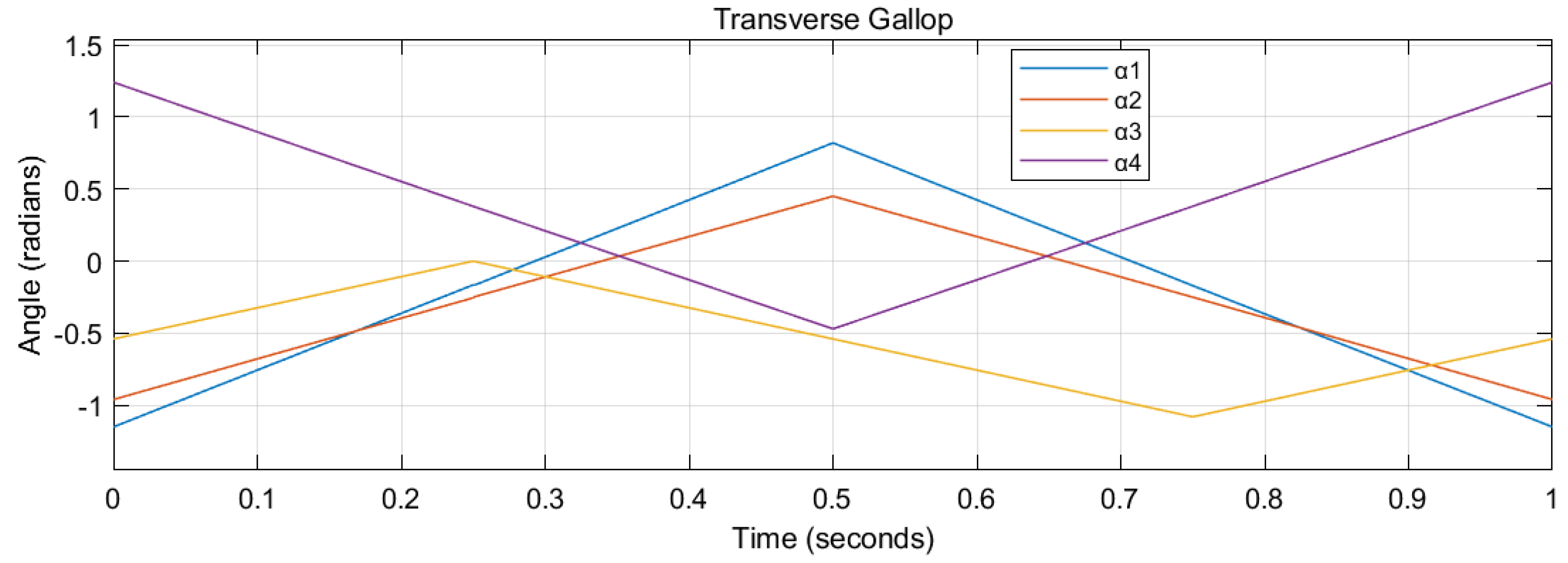
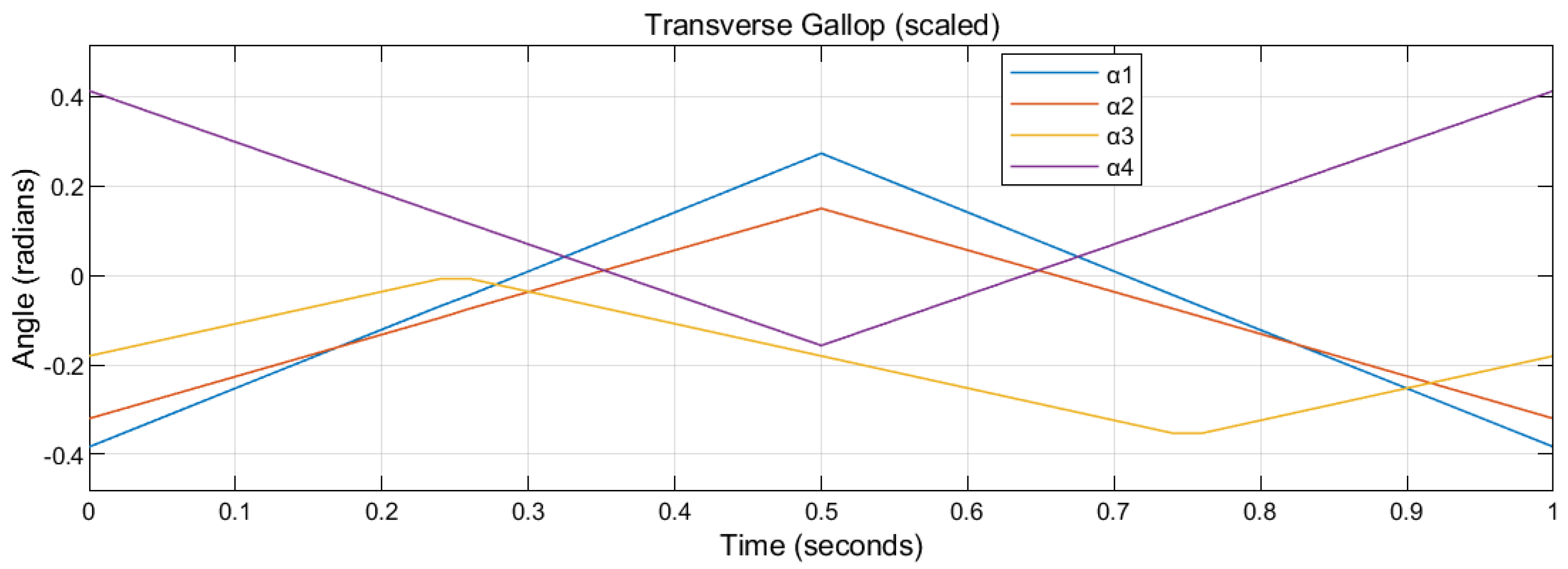
These four gaits, given that the period is 1 s, can be approximated (interpolation) in
Figure 2,
Figure 3,
Figure 4 and
Figure 5, respectively. The abscissa represents the time in a period (0 to 1 s). The ordinate represents the relevant tilting angles,
,
,
, and
, at the corresponding given time point.
Obviously, the condition (11) may not hold for the gaits designed, leading to a singular decoupling matrix. The problems referring to singularities are discussed in the next section.
4. Singular Decoupling Matrix and Gait Modification
The decoupling matrix is required to be invertible while applying feedback linearization. This section discusses the singularity of the decoupling matrix.
The preliminary condition to receive an invertible decoupling matrix is given in (11). However, satisfying (11) does not necessarily mean that the decoupling matrix is invertible.
One may notice that satisfying (11) can also encounter zero angular velocities of the propellers, leading to a singular decoupling matrix. There is other research focusing on the bound-avoidance of the inputs/states [
27], which is beyond the scope of this study.
Also, notice that the necessary and sufficient condition in (11) is an approximation at
. On the other hand, as explained in our previous research [
19], the state
is not a typical equilibrium state. This causes us to visualize the attitudes with the risk of introducing a singular decoupling matrix.
The exact necessary and sufficient condition [
18] to receive an invertible decoupling matrix is
Once
is determined, the unacceptable attitude can be found in
plane by equaling the left side of (15) to 0. The unqualified gaits, leading to the invertible decoupling matrix only in a small attitude region, can be modified by scaling,
The tilting angles are then scaled by in this modification.
Proposition 1. There will always be a positive integer n such that the modified gait by scaling by 1/n produces an invertible decoupling matrix.
Proof of Proposition 1. For a sufficiently large
, we have
Substituting (17) into the left side of (15) yields
which is non-zero, given
, satisfying (15). □
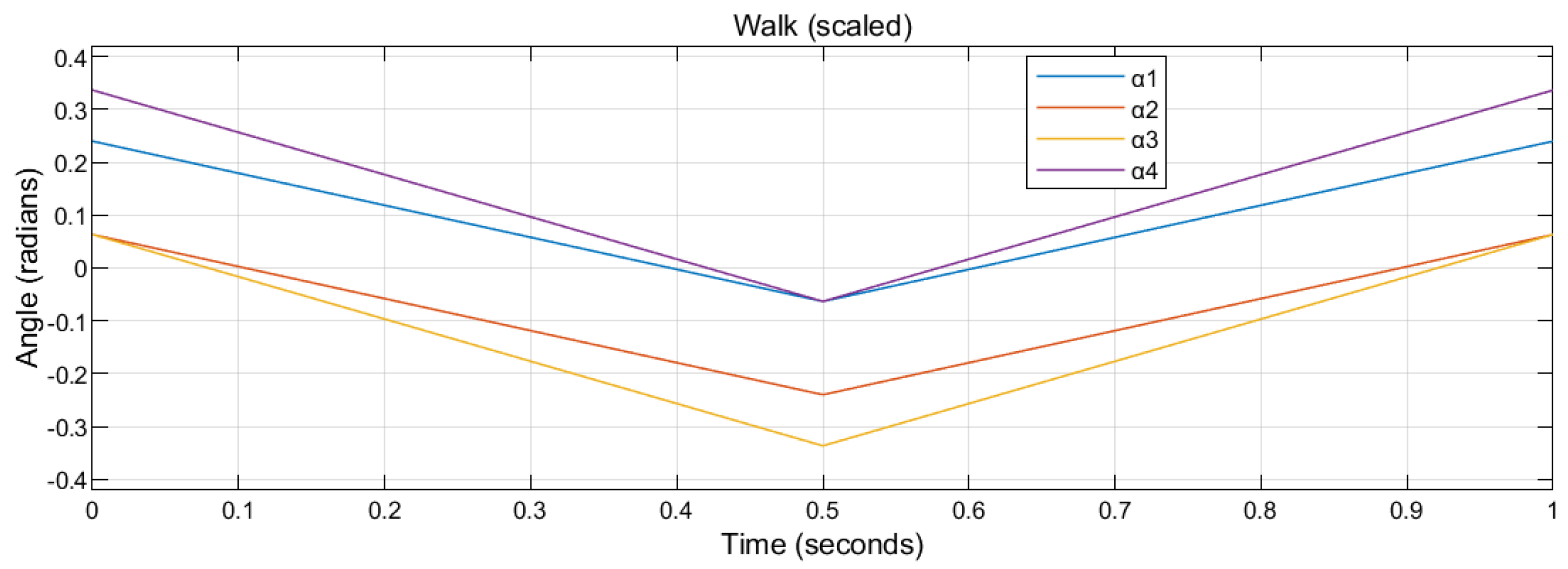
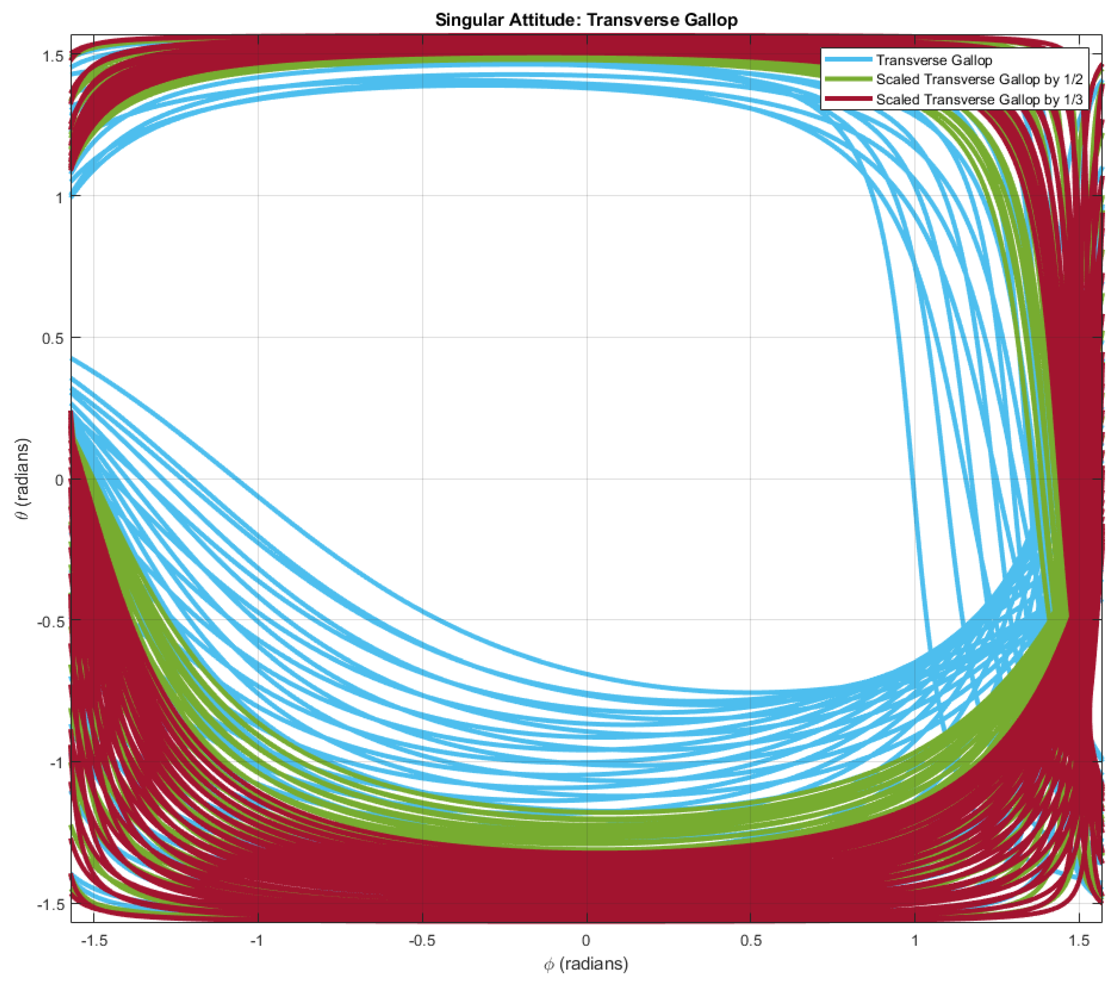
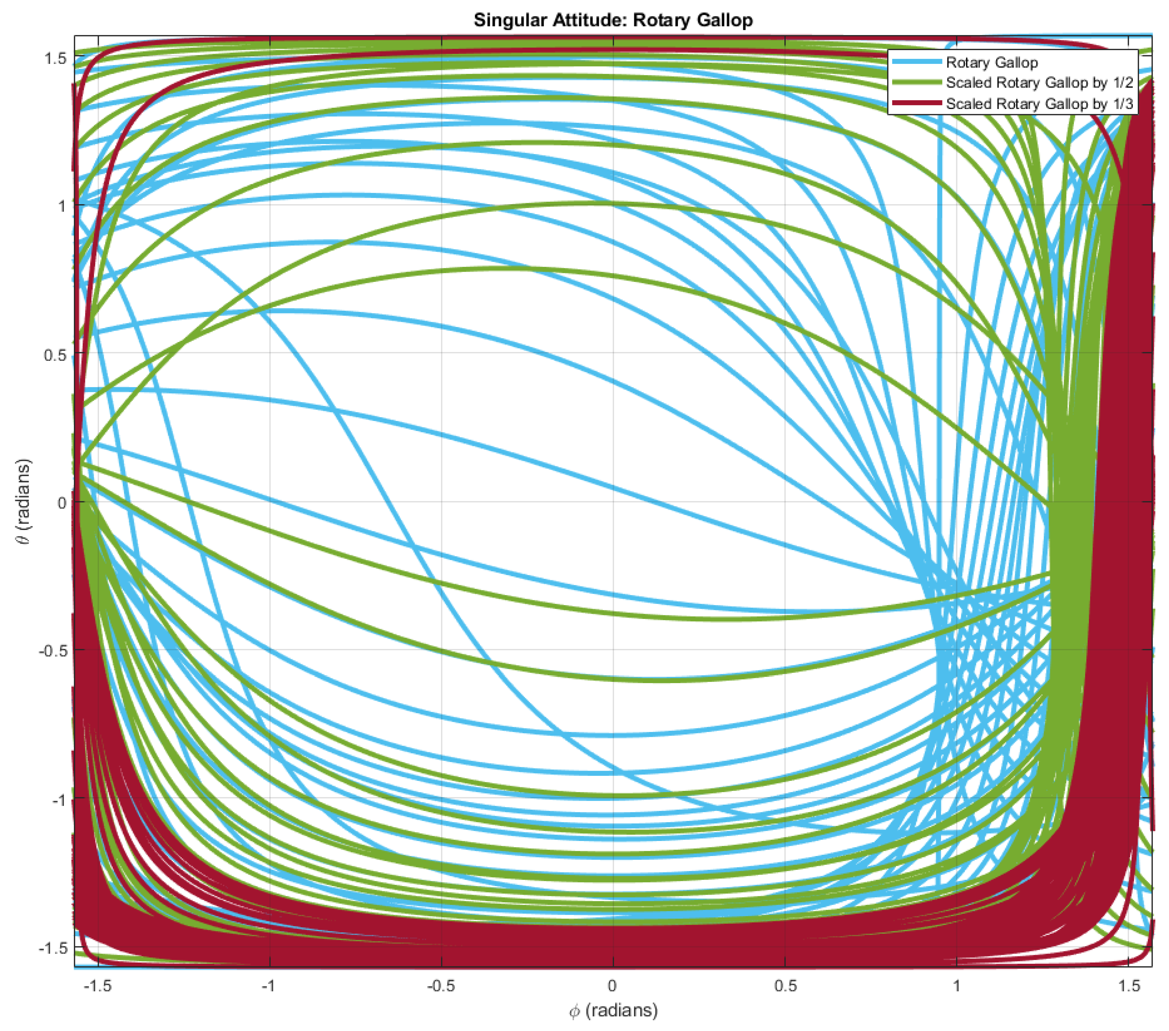
The walk gait, transverse gallop, and rotary gallop gait are scaled by 1/3, respectively, into
Figure 6,
Figure 7 and
Figure 8. Identical to the previous notations, the abscissa represents the time in a period (0 to 1 s). The ordinate represents the relevant tilting angles,
,
,
, and
, at the corresponding given time point.
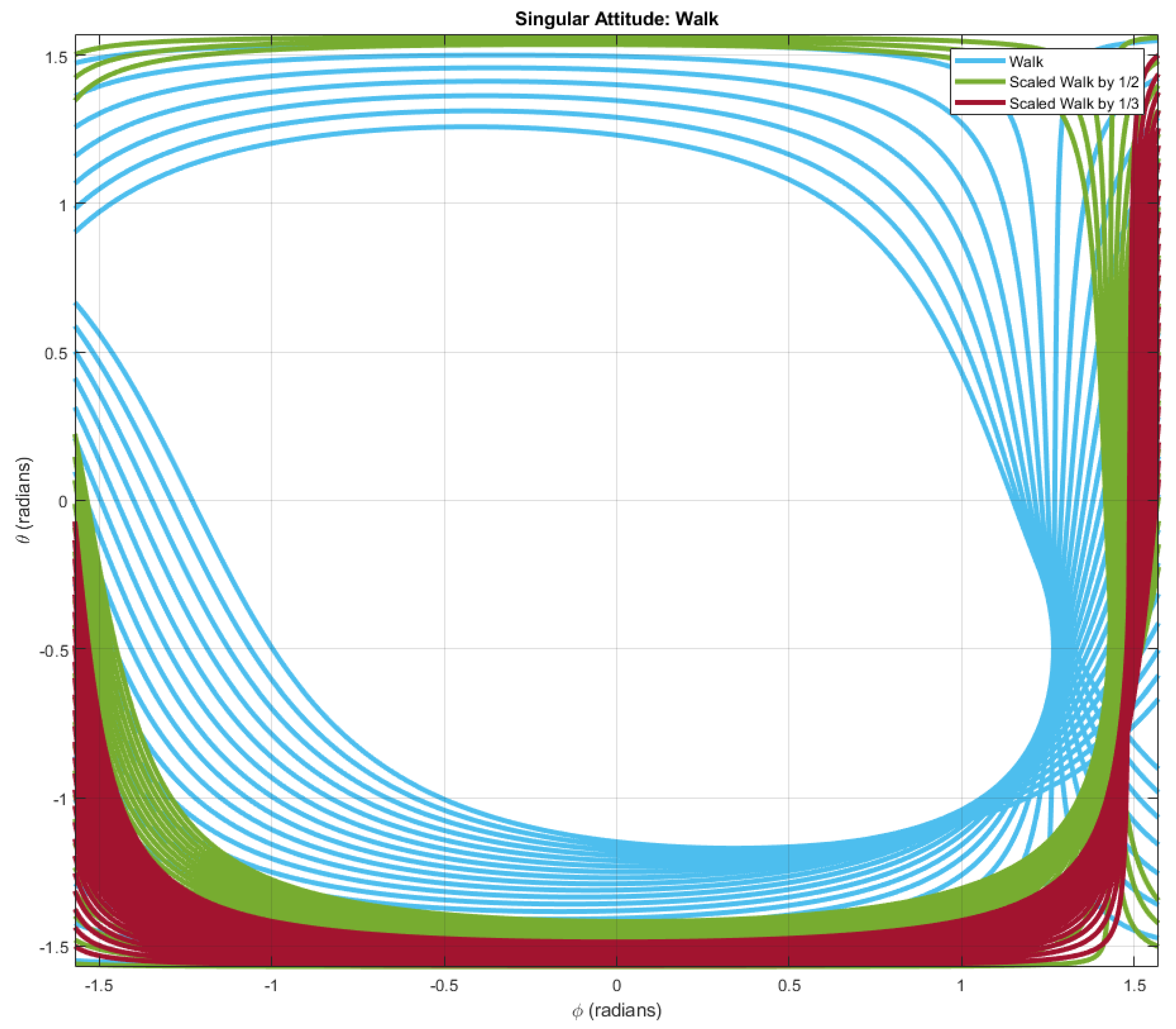
For a given gait, four time-specified tilting angles define the unacceptable attitudes as the attitudes that violate Formula (15); these unacceptable attitudes lead the left side of Formula (15) to zero.
Equaling the left side of Formula (15) to zero, the unacceptable attitudes,
and
, can be tracked by finding the roots, given a determined gait. The unacceptable attitudes in
plane for different scaled walk gaits are plotted in
Figure 9.
Since the attitudes of most flights are near , we evaluate the quality of a gait by finding the distance between and the closest curve of the unacceptable attitudes. For a gait receiving a long distance between and the closest curve of the unacceptable attitudes, the tilt-rotor has a large acceptable attitude region. A gait receiving a short distance between and the closest curve of the unacceptable attitudes in the roll-pitch diagram provides a small acceptable attitude region.
Thus, a gait with a larger distance between and the curve of the unacceptable attitudes is more robust to the attitude; the acceptable attitude region for the tilt-rotor adopting this gait is wider.
It can be found that the acceptable attitude region is enlarging while evenly shrinking the scale of the walk gait. A similar result can also be notably observed in scaled transverse gallop gaits (
Figure 10) and scaled rotary gallop gaits (
Figure 11).
The unreferred gait, run gait, remains identical to the original cat-run gait.
5. Simulation Settings
Similar to our previous research [
19], the references set in this research are the uniform rectilinear motion and the uniform circular motion with zero yaw and zero altitude (
), which are specified as
We adopt this reference since this speed accommodates the cat-trot gait only, which is not preferable to any of the gaits analyzed in this study. The tilt-rotor is then required to track these unbiased references with the relevant gaits.
The absolute value of each initial angular velocity was 300 (rad/s). Each gait is adopted with three different periods (1 (s), 2 (s), and 3 (s)) to track these two references. In addition, the conventional attitude-position decoupler and the modified attitude-position decoupler for a tilt-rotor [
19] are both tested and compared.
The supremum of the dynamic state error in position, after sufficient time, is defined as
where
is the dynamic state error in position defined as
where
and
represent the dynamic state errors along
X and
Y directions, respectively.
The supremum of the dynamic state error in position, after sufficient time, is recorded and compared in each test.
The simulation is conducted in Simulink, MATLAB. Ode3 with sampling time 0.001 (s) is adopted in our solver.
6. Results
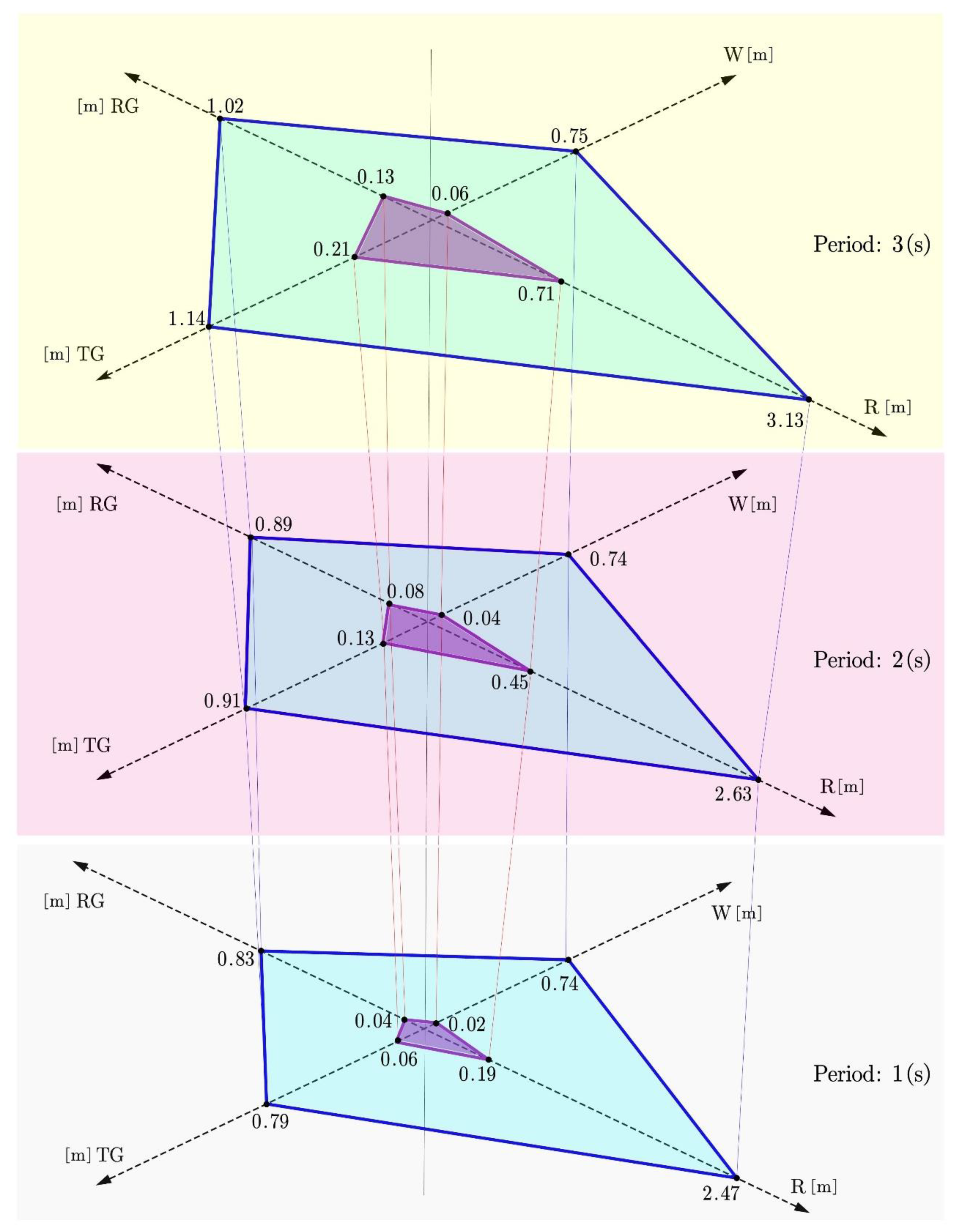
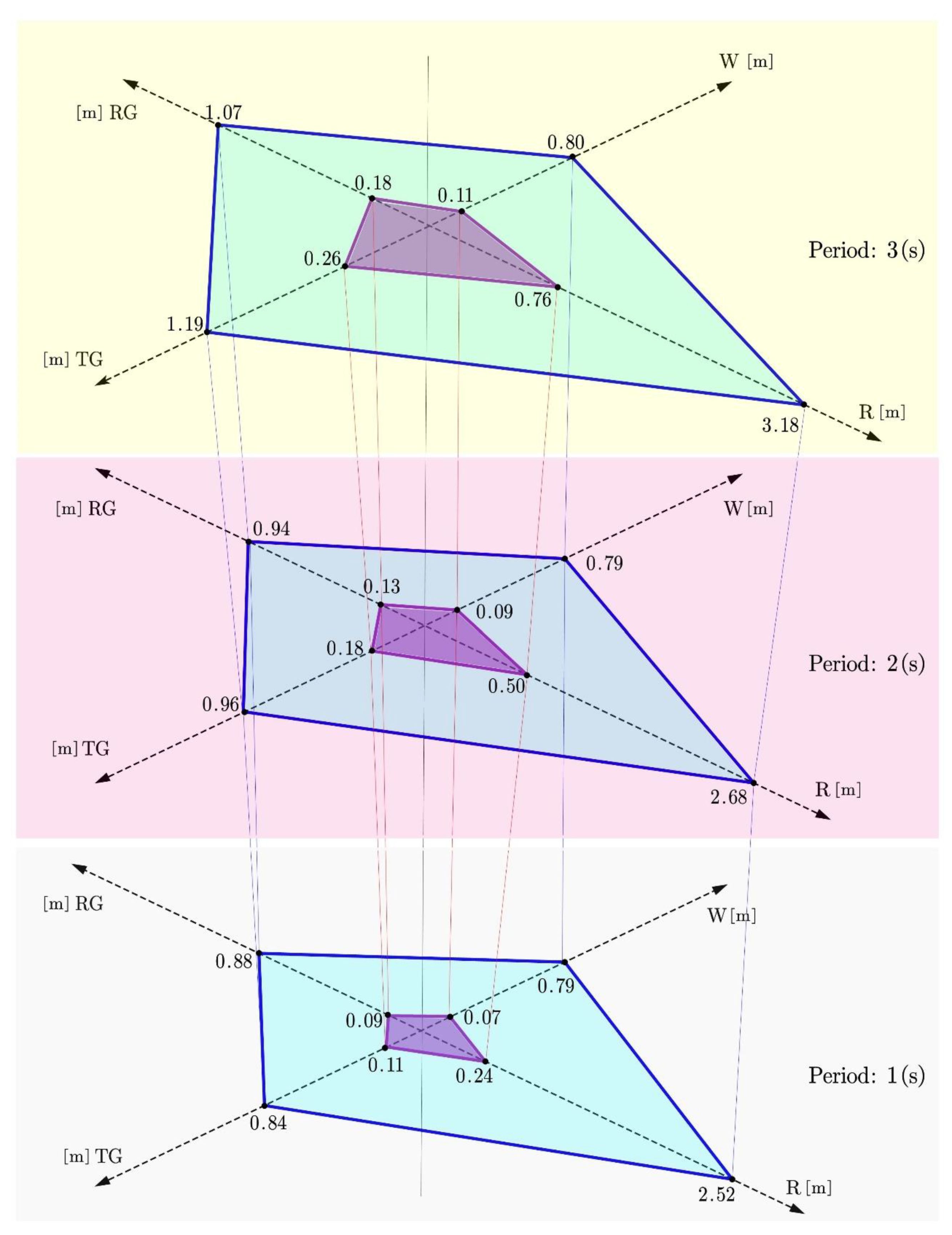
For the first reference, uniform rectilinear motion, the suprema of the dynamic state error (unit: meter), after sufficient time, for different gaits and different periods are concluded in
Figure 12.
The results are classified into 3 sections based on the period of the gaits. They are 1 s (gray), 2 s (red), and 3 s (yellow), respectively. The axis W, R, TG, and RG represents walk gait, run gait, transverse gallop gait, and rotary gallop gait, respectively. The vertexes of the outer quadrilateral (blue) represent the result equipped with the conventional attitude-position decoupler. The vertexes of the inner quadrilateral (purple) represent the result equipped with the modified attitude-position decoupler, (12) and (13).
For example, the “2.47” on the “W” axis on the outer quadrilateral (blue) in “Period: 1 (s)” in
Figure 12 means that the supremum of the dynamic state error, after sufficient time, is 2.47 m, adopting the walk-inspired gait with a period of 1 s equipped with the conventional attitude-position decoupler. The “0.19” on the “W” axis on the inner quadrilateral (purple) in “Period: 1 (s)” in
Figure 12 means that the supremum of the dynamic state error, after sufficient time, is 0.19 m, adopting the walk-inspired gait with a period of 1 s equipped with the modified attitude-position decoupler.
In addition, the result of the simulation with the uniform circular motion is plotted in
Figure 13.
The same notation rule is adopted. Specifically, the results are classified into 3 sections based on the period of the gaits. They are 1 s (gray), 2 s (red), and 3 s (yellow), respectively. The axis W, R, TG, and RG represents walk gait, run gait, transverse gallop gait, and rotary gallop gait, respectively. The vertexes of the outer quadrilateral (blue) represent the result equipped with the conventional attitude-position decoupler. The vertexes of the inner quadrilateral (purple) represents the result equipped with the modified attitude-position decoupler, (12) and (13).
It can be clearly seen that the inner purple quadrilateral is much smaller than the outer blue quadrilateral, which demonstrates that our modified attitude-position decoupler significantly decreases the dynamic state error for all the gaits discussed in this research. This novel attitude-position decoupler is particularly effective for the case suffering from a large dynamic state error equipped with the conventional attitude-position decoupler.
Another interesting result is that the choice of the period influences the dynamic state error. The longer the period is, the larger dynamic state error there tends to be in walk gait, run gait, transverse gallop gait, and rotary gallop gait. The result of the walk gaits is insignificantly influenced by the period settings, while the result in the run gait highly relies on the period settings.
7. Conclusions and Discussions
The four cat gaits, walk gait, run gait, transverse gallop gait, and rotary gallop gait are feasible to be transplanted to solve the gait plan problem for a tilt-rotor. However, walk gait, transverse gallop gait, and rotary gallop gait are required to be modified, e.g., scaling, before being adopted.
The previous research proved that the cat-trot-gait planned tilt-rotor receives the invertible decoupling matrix near zero attitude region analytically. The parallel analytical necessary and sufficient condition to receive a regular decoupling matrix is not straightforward for the four cat gaits, walk gait, run gait, transverse gallop gait, and rotary gallop gait. Thus, this research proposed the singular curves in the roll-pitch diagram to analyze the property of the decoupling matrix for the first time.
Before this article, no systematic methods were put forward to modify a gait, which is liable to introduce a singular decoupling matrix in a tilt-rotor. The scaling method in the gait modification is proven to be feasible in finding a valid gait, liable to lead to the invertible decoupling matrix for the first time; this scaling method tends to enlarge the acceptable attitude zone in the roll-pitch diagram, indicating that this method strengthens the relevant gait.
The modified gaits in this simulation show promising tracking results, where the dynamic state error is acceptable in the tracking problem. Further, the modified walk-inspired gait in this research receives the least suprema of the dynamic state error after sufficient time, while the run-inspired gait receives the largest suprema of the dynamic state error after sufficient time. As for the rest of the gaits analyzed in his research, the modified transverse gallop gait and rotary gallop gait receive similar suprema of the dynamic state error after sufficient time. Beware that the dynamic state error may also be influenced by the maximum tilting angle of each gait, which is not identical in different gaits in this research.
It is not surprising that the modified attitude-position decoupler significantly reduces the dynamic state error for the tilt-rotor for each gait analyzed in this research; we have witnessed similar results in previous research [
19]. This research further verifies the effectiveness of the modified attitude-position decoupler.
The length of the period of the gaits influences the dynamic state error. In general, the longer the period is, the larger dynamic state error there tends to be. Elucidating the underlying mechanism is beyond the scope of this research.
The unique contributions of this research can be concluded as follows: 1. A numerical method (singular curves in the roll-pitch diagram) of analyzing the robustness of the gaits is put forward for the first time. 2. A novel method for modifying the unqualified gaits is created and proven feasible theoretically. 3. The four typical cat-inspired gaits (walk gait, run gait, transverse gallop gait, and rotary gallop gait) are modified to accommodate the tracking problem based on feedback linearization.
Table 1 compares the methods in analyzing the property of the decoupling matrix of the animal-inspired gaits (cat walk/run/transverse gallop/rotary gallop) in this research and of the cat-trot inspired gait in the previous research.
There are several points worth exploring further. Firstly, since the scaling method is the only approach in modifying the gaits in this research, there might be other effective methods with sound mathematical grounds.
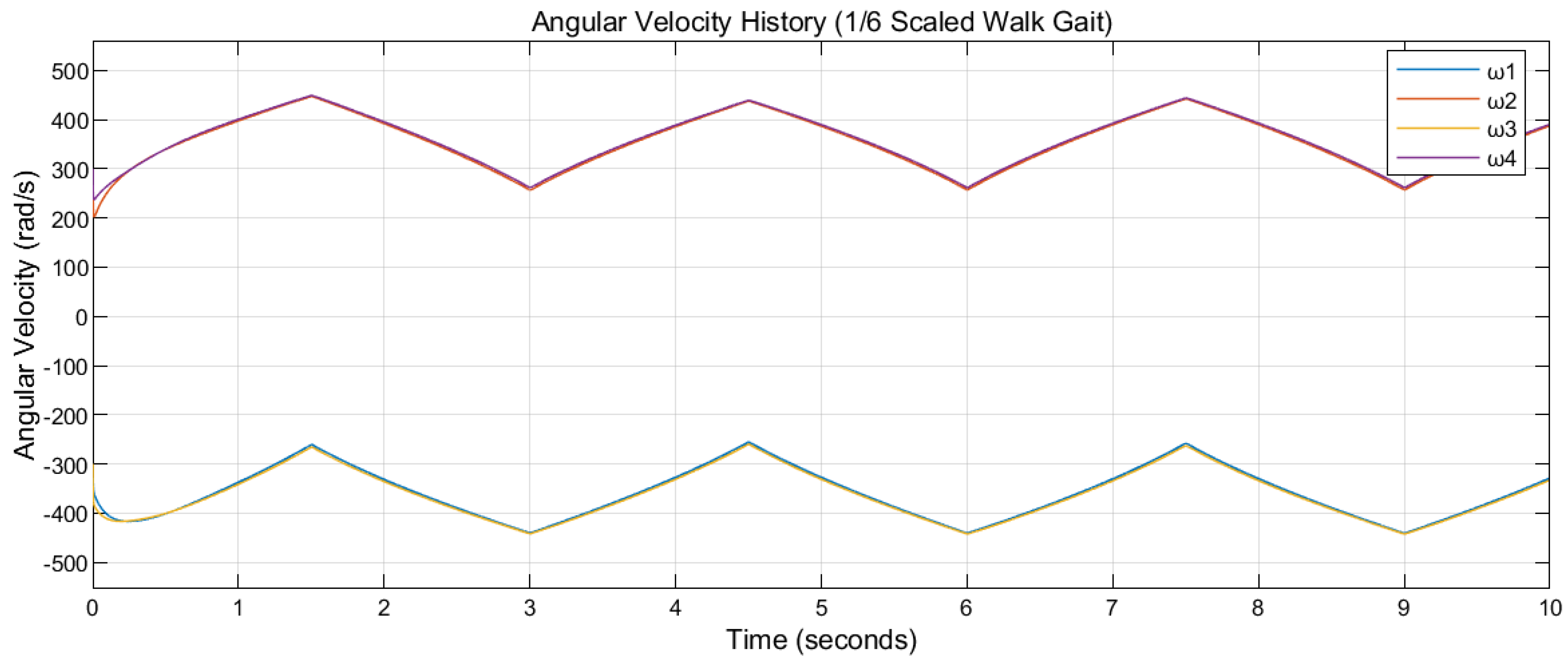
Figure 14 and
Figure 15 display the angular velocity histories while tracking the rectilinear reference defined in Formula (19) with the walk gait scaled by 1/3 and 1/6, respectively. Though the periods of both gaits are identical (3 s), the scale of the tilting angles influences the resulting angular velocities of the propellers of the tilt-rotor. It can be asserted that the desired magnitude of the thrust of each propeller is influenced by the adopted gait.
It can also be found that the robustness of the tilt-rotor increases while scaling. This process, however, sacrifices the lateral force generated by the tilt-rotor. The trade-off between the scaling of the magnitude of the lateral force would be interesting to investigate during further research, as well as a real model to test this rule.


