
Gait Analysis for a Tiltrotor: The Dynamic Invertible Gait


Abstract
:1. Introduction
2. Dynamics of the Tiltrotor
3. Feedback Linearization and Control
3.1. Feedback Linearization
3.2. Third-Order PD Controllers
4. Applicable Gait (Necessary Conditions)
5. Attitude–Altitude Stabilization Test
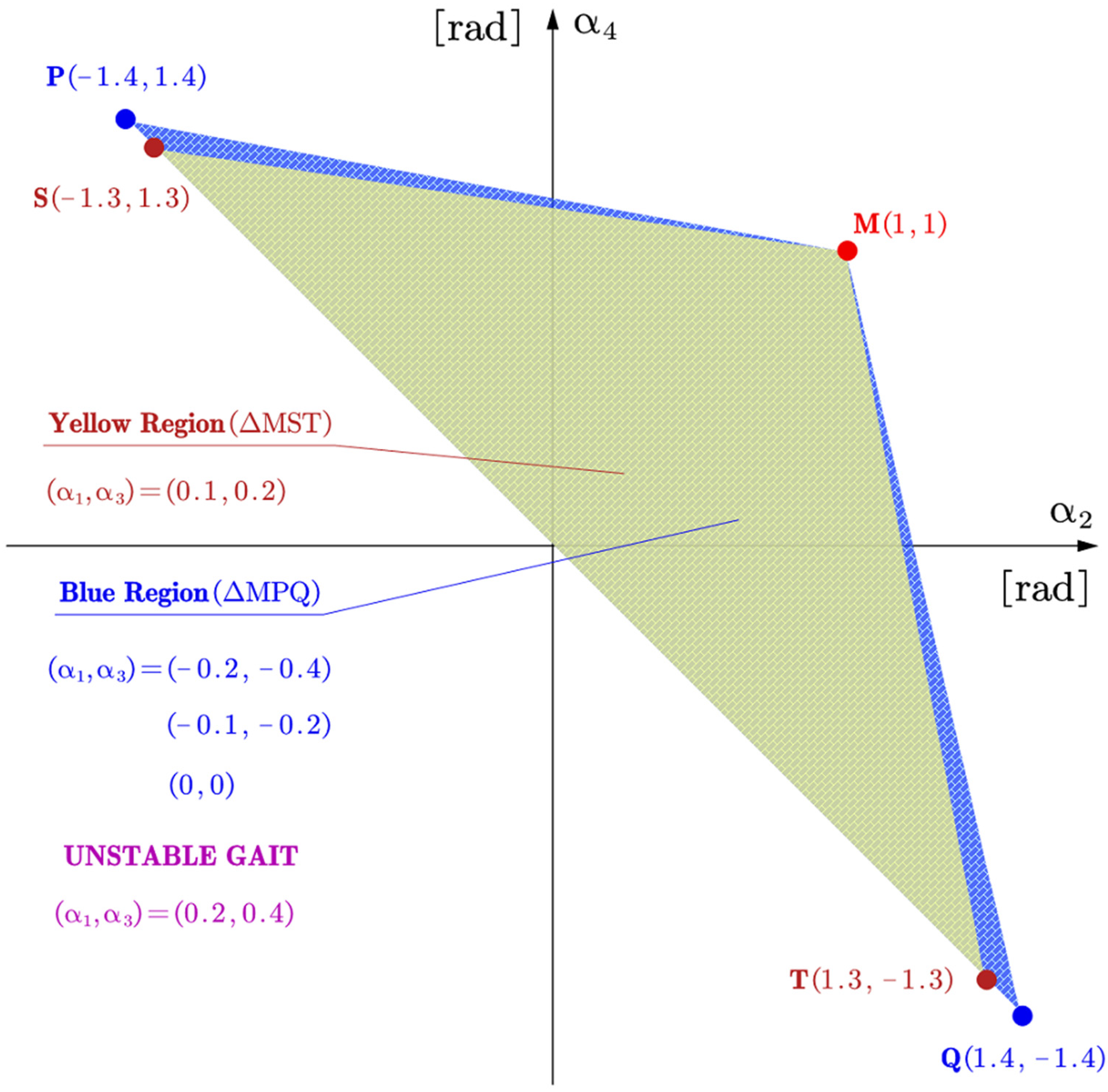
5.1. Restricted Gait Region
5.1.1. Case 1 (Equal)
5.1.2. Case 2 (Half)
5.1.3. Case 3 (Negative)
5.1.4. Case 4 (Negative Half)
5.2. Interested Gait Region and Direction of Exploration
5.2.1. Interested Gait Region
5.2.2. Direction of Exploration
5.3. Attitude–Altitude Control
6. Results
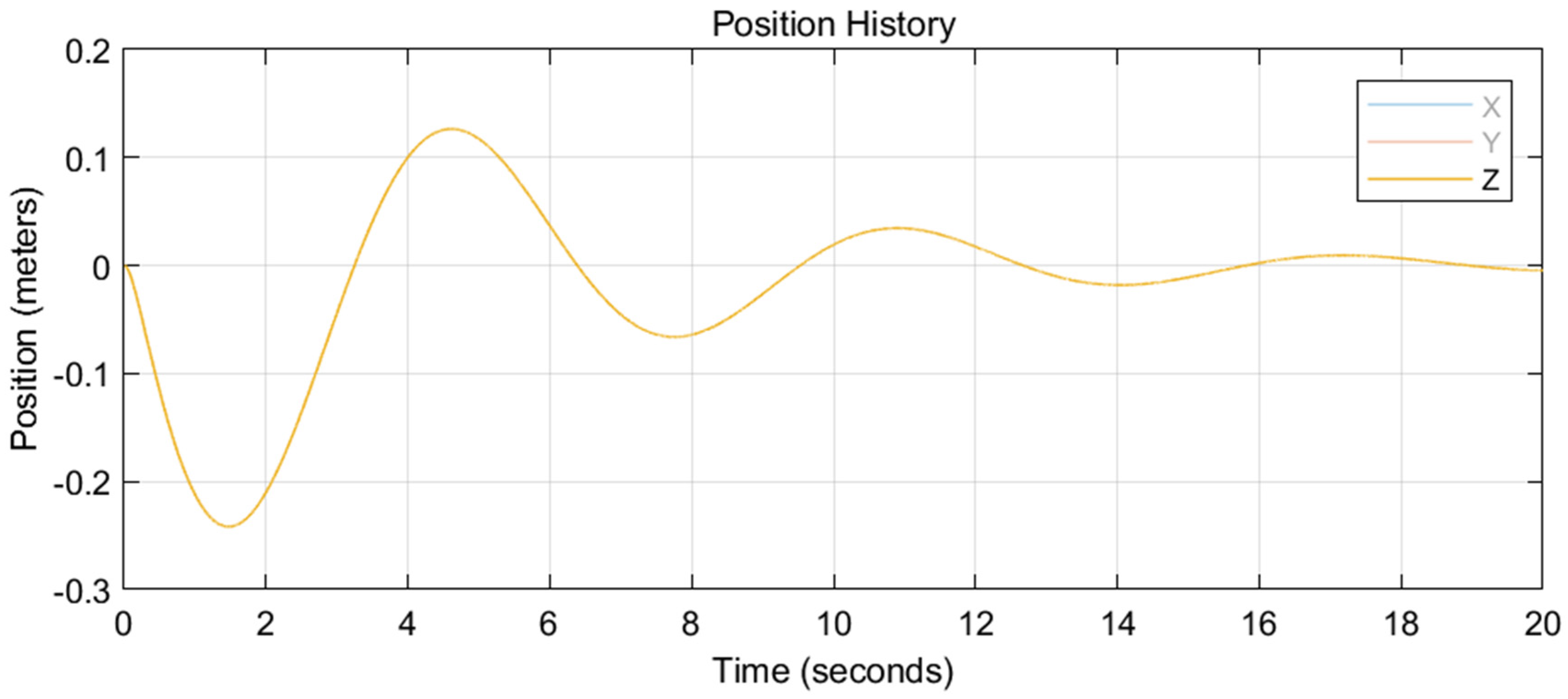
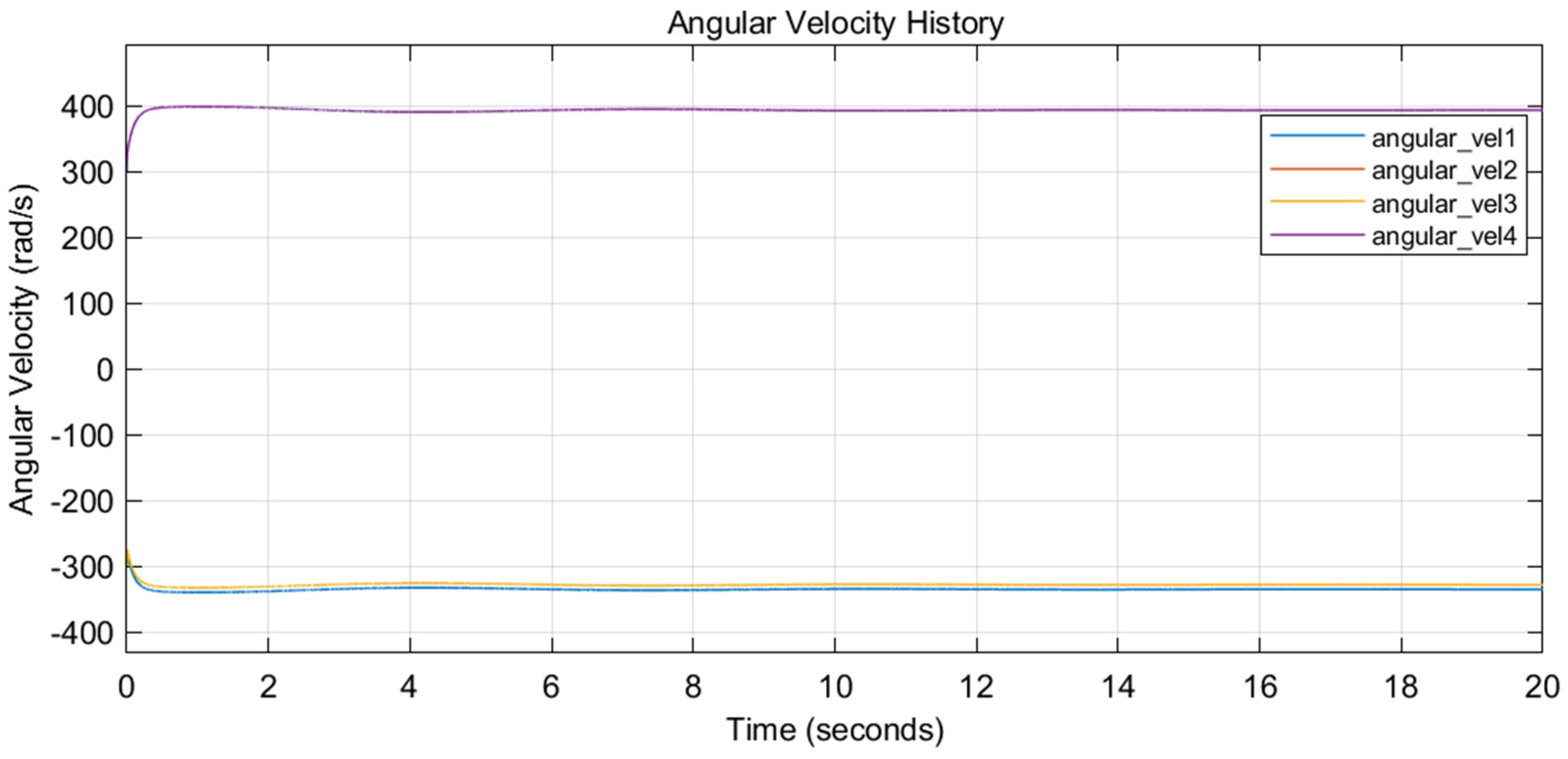
6.1. Flight History
6.1.1. Gait 1
6.1.2. Gait 2
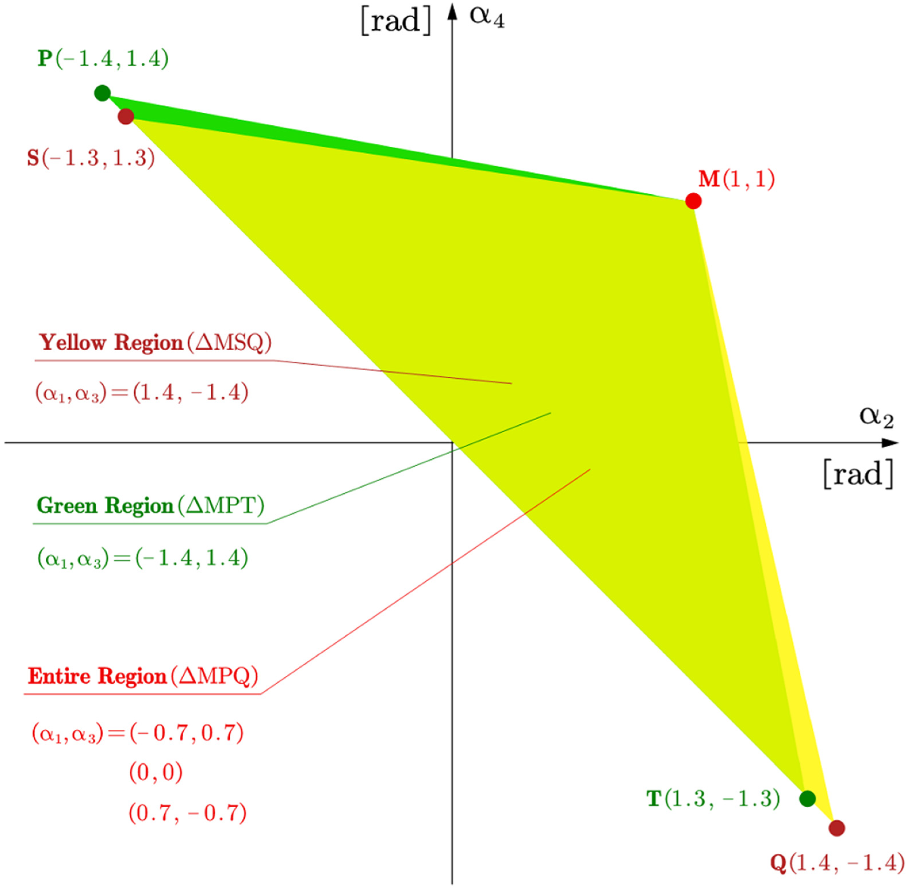
6.2. Applicable Gait (Sufficient Conditions)
6.3. Over-Actuated Control
7. Conclusions and Discussions
Author Contributions
Funding
Institutional Review Board Statement
Informed Consent Statement
Data Availability Statement
Conflicts of Interest
References
- Ryll, M.; Bülthoff, H.H.; Giordano, P.R. Modeling and Control of a Quadrotor UAV with Tilting Propellers. In Proceedings of the IEEE International Conference on Robotics and Automation, Saint Paul, MN, USA, 14–18 May 2012. [Google Scholar]
- Senkul, F.; Altug, E. Adaptive Control of a Tilt-Roll Rotor Quadrotor UAV. In Proceedings of the 2014 International Conference on Unmanned Aircraft Systems, ICUAS 2014, Orlando, FL, USA, 27–30 May 2014. [Google Scholar]
- Senkul, F.; Altug, E. Modeling and Control of a Novel Tilt-Roll Rotor Quadrotor UAV. In Proceedings of the 2013 International Conference on Unmanned Aircraft Systems, ICUAS 2013, Atlanta, GA, USA, 28–31 May 2013. [Google Scholar]
- Nemati, A.; Kumar, M. Modeling and Control of a Single Axis Tilting Quadcopter. In Proceedings of the American Control Conference, Portland, OR, USA, 4–6 June 2014. [Google Scholar]
- Bin Junaid, A.; De Cerio Sanchez, A.D.; Bosch, J.B.; Vitzilaios, N.; Zweiri, Y. Design and Implementation of a Dual-Axis Tilting Quadcopter. Robotics 2018, 7, 65. [Google Scholar] [CrossRef] [Green Version]
- Andrade, R.; Raffo, G.V.; Normey-Rico, J.E. Model Predictive Control of a Tilt-Rotor UAV for Load Transportation. In Proceedings of the 2016 European Control Conference, ECC 2016, Aalborg, Denmark, 29 June–1 July 2016. [Google Scholar]
- Nemati, A.; Kumar, R.; Kumar, M. Stabilizing and Control of Tilting-Rotor Quadcopter in Case of a Propeller Failure. In Proceedings of the ASME 2016 Dynamic Systems and Control Conference, DSCC 2016, Minneapolis, MN, USA, 12–14 October 2016; Volume 1. [Google Scholar]
- Anderson, R.B.; Marshall, J.A.; L’Afflitto, A. Constrained Robust Model Reference Adaptive Control of a Tilt-Rotor Quadcopter Pulling an Unmodeled Cart. IEEE Trans. Aerosp. Electron. Syst. 2021, 57, 39–54. [Google Scholar] [CrossRef]
- Badr, S.; Mehrez, O.; Kabeel, A.E. A Design Modification for a Quadrotor UAV: Modeling, Control and Implementation. Adv. Robot. 2019, 33, 13–32. [Google Scholar] [CrossRef]
- Bhargavapuri, M.; Patrikar, J.; Sahoo, S.R.; Kothari, M. A Low-Cost Tilt-Augmented Quadrotor Helicopter: Modeling and Control. In Proceedings of the 2018 International Conference on Unmanned Aircraft Systems, ICUAS 2018, Dallas, TX, USA, 12–15 June 2018. [Google Scholar]
- Badr, S.; Mehrez, O.; Kabeel, A.E. A Novel Modification for a Quadrotor Design. In Proceedings of the 2016 International Conference on Unmanned Aircraft Systems, ICUAS 2016, Arlington, VA, USA, 7–10 June 2016. [Google Scholar]
- Jiang, X.-Y.; Su, C.-L.; Xu, Y.-P.; Liu, K.; Shi, H.-Y.; Li, P. An Adaptive Backstepping Sliding Mode Method for Flight Attitude of Quadrotor UAVs. J. Cent. South Univ. 2018, 25, 616–631. [Google Scholar] [CrossRef]
- Jin, S.; Kim, J.; Kim, J.W.; Bae, J.H.; Bak, J.; Kim, J.; Seo, T.W. Back-Stepping Control Design for an Underwater Robot with Tilting Thrusters. In Proceedings of the 17th International Conference on Advanced Robotics, ICAR 2015, Istanbul, Turkey, 27–31 July 2015. [Google Scholar]
- Kadiyam, J.; Santhakumar, M.; Deshmukh, D.; Seo, T.W. Design and Implementation of Backstepping Controller for Tilting Thruster Underwater Robot. In Proceedings of the International Conference on Control, Automation and Systems, PyeongChang, Korea, 17–20 October 2018; Volume 2018. [Google Scholar]
- Scholz, G.; Popp, M.; Ruppelt, J.; Trommer, G.F. Model Independent Control of a Quadrotor with Tiltable Rotors. In Proceedings of the IEEE/ION Position, Location and Navigation Symposium, PLANS 2016, Savannah, GA, USA, 11–14 April 2016. [Google Scholar]
- Phong Nguyen, N.; Kim, W.; Moon, J. Observer-Based Super-Twisting Sliding Mode Control with Fuzzy Variable Gains and Its Application to Overactuated Quadrotors. In Proceedings of the IEEE Conference on Decision and Control, Miami, FL, USA, 17–19 December 2018; Volume 2018. [Google Scholar]
- Kumar, R.; Nemati, A.; Kumar, M.; Sharma, R.; Cohen, K.; Cazaurang, F. Tilting-Rotor Quadcopter for Aggressive Flight Maneuvers Using Differential Flatness Based Flight Controller. In Proceedings of the ASME 2017 Dynamic Systems and Control Conference, DSCC 2017, Tysons, VA, USA, 11–13 October 2017; Volume 3. [Google Scholar]
- Saif, A.-W.A. Feedback Linearization Control of Quadrotor with Tiltable Rotors under Wind Gusts. Int. J. Adv. Appl. Sci. 2017, 4, 150–159. [Google Scholar] [CrossRef]
- Offermann, A.; Castillo, P.; De Miras, J.D. Control of a PVTOL* with Tilting Rotors*. In Proceedings of the 2019 International Conference on Unmanned Aircraft Systems, ICUAS 2019, Atlanta, GA, USA, 11–14 June 2019. [Google Scholar]
- Rajappa, S.; Bulthoff, H.H.; Odelga, M.; Stegagno, P. A Control Architecture for Physical Human-UAV Interaction with a Fully Actuated Hexarotor. In Proceedings of the IEEE International Conference on Intelligent Robots and Systems, Vancouver, BC, Canada, 24–28 September 2017; Volume 2017. [Google Scholar]
- Scholz, G.; Trommer, G.F. Model Based Control of a Quadrotor with Tiltable Rotors. Gyroscopy Navig. 2016, 7, 72–81. [Google Scholar] [CrossRef]
- Ryll, M.; Bülthoff, H.H.; Giordano, P.R. A Novel Overactuated Quadrotor Unmanned Aerial Vehicle: Modeling, Control, and Experimental Validation. IEEE Trans. Control Syst. Technol. 2015, 23, 540–556. [Google Scholar] [CrossRef] [Green Version]
- Elfeky, M.; Elshafei, M.; Saif, A.W.A.; Al-Malki, M.F. Quadrotor Helicopter with Tilting Rotors: Modeling and Simulation. In Proceedings of the 2013 World Congress on Computer and Information Technology, WCCIT 2013, Sousse, Tunisia, 22–24 June 2013. [Google Scholar]
- Park, S.; Lee, J.; Ahn, J.; Kim, M.; Her, J.; Yang, G.H.; Lee, D. ODAR: Aerial Manipulation Platform Enabling Omnidirectional Wrench Generation. IEEE/ASME Trans. Mechatron. 2018, 23, 1907–1918. [Google Scholar] [CrossRef]
- Magariyama, T.; Abiko, S. Seamless 90-Degree Attitude Transition Flight of a Quad Tilt-Rotor UAV under Full Position Control. In Proceedings of the IEEE/ASME International Conference on Advanced Intelligent Mechatronics, AIM, Boston, MA, USA, 6–9 July 2020; Volume 2020. [Google Scholar]
- Falanga, D.; Kleber, K.; Mintchev, S.; Floreano, D.; Scaramuzza, D. The Foldable Drone: A Morphing Quadrotor That Can Squeeze and Fly. IEEE Robot. Autom. Lett. 2019, 4, 209–216. [Google Scholar] [CrossRef] [Green Version]
- Lu, D.; Xiong, C.; Zeng, Z.; Lian, L. Adaptive Dynamic Surface Control for a Hybrid Aerial Underwater Vehicle with Parametric Dynamics and Uncertainties. IEEE J. Ocean. Eng. 2020, 45, 740–758. [Google Scholar] [CrossRef]
- Antonelli, G.; Cataldi, E.; Arrichiello, F.; Giordano, P.R.; Chiaverini, S.; Franchi, A. Adaptive Trajectory Tracking for Quadrotor MAVs in Presence of Parameter Uncertainties and External Disturbances. IEEE Trans. Control Syst. Technol. 2018, 26, 248–254. [Google Scholar] [CrossRef]
- Lee, D.; Jin Kim, H.; Sastry, S. Feedback Linearization vs. Adaptive Sliding Mode Control for a Quadrotor Helicopter. Int. J. Control Autom. Syst. 2009, 7, 419–428. [Google Scholar] [CrossRef]
- Al-Hiddabi, S.A. Quadrotor Control Using Feedback Linearization with Dynamic Extension. In Proceedings of the 2009 6th International Symposium on Mechatronics and its Applications, Sharjah, United Arab Emirates, 23–26 March 2009; pp. 1–3. [Google Scholar]
- Mukherjee, P.; Waslander, S. Direct Adaptive Feedback Linearization for Quadrotor Control. In Proceedings of the AIAA Guidance, Navigation, and Control Conference, Minneapolis, MN, USA, 13–16 August 2012. [Google Scholar]
- Rajappa, S.; Ryll, M.; Bulthoff, H.H.; Franchi, A. Modeling, Control and Design Optimization for a Fully-Actuated Hexarotor Aerial Vehicle with Tilted Propellers. In Proceedings of the IEEE International Conference on Robotics and Automation, Seattle, WA, USA, 26–30 May 2015; Volume 2015. [Google Scholar]
- Dunham, W.; Petersen, C.; Kolmanovsky, I. Constrained Control for Soft Landing on an Asteroid with Gravity Model Uncertainty. In Proceedings of the American Control Conference, Boston, MA, USA, 6–8 July 2016; Volume 2016. [Google Scholar]
- McDonough, K.; Kolmanovsky, I. Controller State and Reference Governors for Discrete-Time Linear Systems with Pointwise-in-Time State and Control Constraints. In Proceedings of the American Control Conference, Chicago, IL, USA, 1–3 July 2015; Volume 2015. [Google Scholar]
- Kolmanovsky, I.; Kalabić, U.; Gilbert, E. Developments in Constrained Control Using Reference Governors. IFAC Proc. 2012, 4, 282–290. [Google Scholar] [CrossRef]
- Bemporad, A. Reference Governor for Constrained Nonlinear Systems. IEEE Trans. Autom. Control 1998, 43, 415–419. [Google Scholar] [CrossRef] [Green Version]
- Shen, Z.; Ma, Y.; Tsuchiya, T. Stability Analysis of a Feedback-Linearization-Based Controller with Saturation: A Tilt Vehicle with the Penguin-Inspired Gait Plan. arXiv 2021, arXiv:2111.14456. [Google Scholar]
- Franchi, A.; Carli, R.; Bicego, D.; Ryll, M. Full-Pose Tracking Control for Aerial Robotic Systems with Laterally Bounded Input Force. IEEE Trans. Robot. 2018, 34, 534–541. [Google Scholar] [CrossRef] [Green Version]
- Horla, D.; Hamandi, M.; Giernacki, W.; Franchi, A. Optimal Tuning of the Lateral-Dynamics Parameters for Aerial Vehicles with Bounded Lateral Force. IEEE Robot. Autom. Lett. 2021, 6, 3949–3955. [Google Scholar] [CrossRef]
- Shen, Z.; Tsuchiya, T. State Drift and Gait Plan in Feedback Linearization Control of A Tilt Vehicle. arXiv 2021, arXiv:2111.04307. [Google Scholar]
- Chernova, S.; Veloso, M. An Evolutionary Approach to Gait Learning for Four-Legged Robots. In Proceedings of the 2004 IEEE/RSJ International Conference on Intelligent Robots and Systems (IROS), Sendai, Japan, 28 September–2 October 2004; Volume 3. [Google Scholar]
- Bennani, M.; Giri, F. Dynamic Modelling of a Four-Legged Robot. J. Intell. Robot. Syst. Theory Appl. 1996, 17, 419–428. [Google Scholar] [CrossRef]
- Talebi, S.; Poulakakis, I.; Papadopoulos, E.; Buehler, M. Quadruped Robot Running with a Bounding Gait. In Experimental Robotics VII; Rus, D., Singh, S., Eds.; Springer: Berlin/Heidelberg, Germany, 2007. [Google Scholar]
- Lewis, M.A.; Bekey, G.A. Gait Adaptation in a Quadruped Robot. Auton. Robot. 2002, 12, 301–312. [Google Scholar] [CrossRef]
- Hirose, S. A Study of Design and Control of a Quadruped Walking Vehicle. Int. J. Robot. Res. 1984, 3, 113–133. [Google Scholar] [CrossRef]
- Luukkonen, T. Modelling and Control of Quadcopter. Indep. Res. Proj. Appl. Math. 2011, 22, 22. [Google Scholar]
- Goodarzi, F.A.; Lee, D.; Lee, T. Geometric Adaptive Tracking Control of a Quadrotor Unmanned Aerial Vehicle on SE(3) for Agile Maneuvers. J. Dyn. Syst. Meas. Control 2015, 137, 091007. [Google Scholar] [CrossRef] [Green Version]
- Shi, X.-N.; Zhang, Y.-A.; Zhou, D. A Geometric Approach for Quadrotor Trajectory Tracking Control. Int. J. Control 2015, 88, 2217–2227. [Google Scholar] [CrossRef]
- Lee, T.; Leok, M.; McClamroch, N.H. Nonlinear Robust Tracking Control of a Quadrotor UAV on SE(3): Nonlinear Robust Tracking Control of a Quadrotor UAV. Asian J. Control 2013, 15, 391–408. [Google Scholar] [CrossRef] [Green Version]
- Shen, Z.; Tsuchiya, T. Singular Zone in Quadrotor Yaw-Position Feedback Linearization. arXiv 2021, arXiv:2110.07179. [Google Scholar]
- Mistier, V.; Benallegue, A.; M’Sirdi, N.K. Exact Linearization and Noninteracting Control of a 4 Rotors Helicopter via Dynamic Feedback. In Proceedings of the IEEE International Workshop on Robot and Human Interactive Communication, Paris, France, 18–21 September 2001; pp. 586–593. [Google Scholar]
- Das, A.; Subbarao, K.; Lewis, F. Dynamic Inversion with Zero-Dynamics Stabilisation for Quadrotor Control. IET Control Theory Appl. 2009, 3, 303–314. [Google Scholar] [CrossRef] [Green Version]


Publisher’s Note: MDPI stays neutral with regard to jurisdictional claims in published maps and institutional affiliations. |
© 2022 by the authors. Licensee MDPI, Basel, Switzerland. This article is an open access article distributed under the terms and conditions of the Creative Commons Attribution (CC BY) license (https://creativecommons.org/licenses/by/4.0/).
Share and Cite
Shen, Z.; Tsuchiya, T. Gait Analysis for a Tiltrotor: The Dynamic Invertible Gait. Robotics 2022, 11, 33. https://doi.org/10.3390/robotics11020033
Shen Z, Tsuchiya T. Gait Analysis for a Tiltrotor: The Dynamic Invertible Gait. Robotics. 2022; 11(2):33. https://doi.org/10.3390/robotics11020033
Chicago/Turabian StyleShen, Zhe, and Takeshi Tsuchiya. 2022. "Gait Analysis for a Tiltrotor: The Dynamic Invertible Gait" Robotics 11, no. 2: 33. https://doi.org/10.3390/robotics11020033
APA StyleShen, Z., & Tsuchiya, T. (2022). Gait Analysis for a Tiltrotor: The Dynamic Invertible Gait. Robotics, 11(2), 33. https://doi.org/10.3390/robotics11020033