Article

Faster than Real-Time Surface Pose Estimation with Application to Autonomous Robotic Grasping

1
Electrical and Computer Engineering Department, University of Central Florida (UCF), Orlando, FL 32816, USA
2
Electrical and Computer Engineering Department, NSTC at UCF, Orlando, FL 32816, USA
*
Author to whom correspondence should be addressed.
Robotics 2022, 11(1), 7; https://doi.org/10.3390/robotics11010007
Submission received: 13 September 2021 / Revised: 12 December 2021 / Accepted: 29 December 2021 / Published: 2 January 2022
(This article belongs to the Section Intelligent Robots and Mechatronics)

Abstract

:
Motivated by grasp planning applications within cluttered environments, this paper presents a novel approach to performing real-time surface segmentations of never-before-seen objects scattered across a given scene. This approach utilizes an input 2D depth map, where a first principles-based algorithm is utilized to exploit the fact that continuous surfaces are bounded by contours of high gradient. From these regions, the associated object surfaces can be isolated and further adapted for grasp planning. This paper also provides details for extracting the six-DOF pose for an isolated surface and presents the case of leveraging such a pose to execute planar grasping to achieve both force and torque closure. As a consequence of the highly parallel software implementation, the algorithm is shown to outperform prior approaches across all notable metrics and is also shown to be invariant to object rotation, scale, orientation relative to other objects, clutter, and varying degree of noise. This allows for a robust set of operations that could be applied to many areas of robotics research. The algorithm is faster than real time in the sense that it is nearly two times faster than the sensor rate of 30 fps.

1. Introduction

Research surrounding robot grasp planning has accelerated tremendously as a result of recent advancements in areas relating to computer vision, perception-based sensors, and mechanical systems. While these strides have paved the way for more robust grasping methods, limitations in computational prowess and control strategies continue to constrain grasp synthesis to predefined grasping patterns or computationally heavy grasping algorithms that are infeasible for day-to-day real-time operations. Moreover, the demand for a more robust autonomous grasping algorithm, which can manipulate arbitrary objects within unstructured environments, has significantly increased within the past few years as economic pressures push more robots into the day-to-day activities of the marketplace. This is made even more necessary and critical in the field of assistive robotics where an aging generation will require the aid of machines to fulfill their daily needs. While achieving human-level grasping requires the consolidation of a vast array of research domains, ranging from biology, physics, engineering, and computer science, this research seeks a first-principles-based approach to identify graspable features within a scene for object manipulation. It is shown that the most primitive elements of these features, edges and object surfaces, constitute enough information to immobilize the associated object. Thus, the primary objective of this research is to present a faster-than-real-time framework for segmenting object surfaces from a depth image. Furthermore, a six-DOF surface pose is computed for specified surface segments and serves as a framework to ease the use of generating the appropriate grasping configuration necessary to manipulate the desired object.
According to Sahbani [1], grasp algorithms can be separated into analytical and empirical techniques. Sahbani determines that an analytical grasping approach must be dependent on a geometric, kinematic, and/or dynamic formulation to immobilize an object. While analytical approaches provide guarantees regarding positioning and kinematic grasping execution, inconsistencies and ambiguities regarding robot modeling and sensor data, however, undermine their effectiveness. This is further exacerbated by the computationally expensive algorithms which yield error-prone kinematic/dynamic approximations during grasp synthesis. In contrast, an empirical approach, also known as a data-driven approach, avoids the heavy computation needed to process the mathematical and physical models by mimicking human grasping strategies derived from predetermined objects or geometric shapes. Bohg et al. [2] further classify these empirical objects into known, familiar, and unknown categories. To summarize, both known and familiar objects are dependent on querying a grasping database for supported grasping strategies in the presence of a known shape. Unknown objects, on the other hand, are reliant on identifying features that could be re-interpreted as primitive shapes that are utilized as potential grasping candidates. Consequently, the empirical approach is wholly reliant on a representative model for associating an arbitrary object with a set of grasping candidates. Nevertheless, Refs. [3,4,5] present robust techniques for representing arbitrary objects as a set of geometric primitives which, in turn, are investigated as potential grasping strategies. Detry et al. [6] advance this approach by encapsulating a bounding box around a desired object and then initiate grasping given a set of intersection rays projected from the bounding region. This method disassociates the need to infer the overall shape of the object, instead relying on a computationally heavy mean of sampling surface boundaries. In contrast, Kroemer et al. [7] rely on a kernel method approach to encode grasping patterns for the portions of an object’s surface that are most commonly grasped. This approach greatly reduces the time taken to infer grasping candidates from the surface of the entire object. Furthermore, Kopicki et al. [8] build on this work by defining a similarity measure between never seen before and previously sampled surfaces. As such, grasp prototypes may be transferable across locally correlated object typologies. Although these approaches improve performance over prior methods, they remain incapable of achieving real-time performance. Detry et al. [6] note that it takes 18 s on average to match grasping prototype against candidates on a single object.
The seminal work of Saxena et al. [9] on the identification of grasp points using visual data has paved the way for many other data-driven approaches in the robotic field. These approaches are distinguished by the format in which they represent input data and output grasp [9,10,11]. Providing grasping points, oriented 2D rectangles, or the 6D pose of specific end-effectors, are key examples. The scale and type (synthetic/real world) of the training data are also varied in the literature [12,13,14]. However, it is noticeable that a common key feature among most of the recent approaches is focusing solely on either a specific gripper solution or a specific grasping policy, which makes such approaches difficult to adapt to other standard grippers and generic environments [15,16,17]. An interesting technique for grasping novel objects using tactile sensors in the fingers is presented in [18].
Recently, Jabalameli and Behal [19] proposed a novel solution for generating a grasping configuration for unknown objects within unstructured scenes. The proposed framework searches for sharp discontinuities or local maxima within a depth image for potential contact candidates to perform a planar grasp. Incidentally, these features are characteristic of boundaries and edges where force closure principles could be applied. Moreover, observing human grasping reveals that people tend to grasp objects by contacting edges and corners [20]. This allows for greater grasping stability by permitting a larger wrench convex. Consequently, Ref. [19] goes on to rely solely on a 2D depth image to extract potential contact set-points instead of relying on clustering to analyze 3D point-cloud coordinates. While such an approach provides effective contact points needed to immobilize an unknown object, it is unable to perform in real-time due to inefficient computational procedures. In addition, because of noise and other inconsistencies within a depth frame, the pixel-level approximation was attributed to significant errors which resulted in inconsistent grasping proposals. Finally, because of the algorithm simplifying assumptions such as avoidance of contour formation, the potential grasping regions were needlessly constrained to parallel edges which therefore constrain grasping configurations to two-fingered grippers.
This paper proposes a novel (faster than) real-time segmentation framework which builds upon the established algorithm of Jabalameli and Behal [19]. To clarify, surface segmentation is defined as the grouping of individual faces of objects within a scene. Consequently, the proposed approach can generate contours bounding object surfaces within a scene, which has the potential to permit an N-fingered grasping configuration to immobilize and manipulate unknown objects within unstructured environments. In addition, this approach establishes a novel means of assessing additional potential grasping candidates by simply altering a camera-in-hand end-effector position and orientation in real time. While our approach relies on an empirical foundation for deriving graspable features for unseen objects, it abstracts the grasping dynamics from the physical object by reducing an object to a set of closed contours. As such, our algorithm requires no prior knowledge of objects within a scene while maintaining a faster-than-real-time and consistent performance that cannot be obtained by an analytical approach. Akin to [19], our algorithm remains solely reliant on a 2D depth stream to produce potential grasping configurations without the need to perform complex clustering algorithms on 3D point-cloud data. Instead, a set of simple transformations is applied to a depth image to obtain a list of surface contours with poses, rendering enough information to achieve planar grasping. The real-time video demonstration shown in [21] illustrates the proposed surface segmentation approach being applied to a real-world data stream.
This paper is organized as follows. Section 2 lays out the details of the system inputs and outputs. This is followed by Section 3, which presents the segmenting algorithm used to identify object contours bounding object surfaces within a depth scene and further introduces the robustification measures needed to mitigate external perturbations that may arise when working with real-world measurements. Section 4 presents the details of the underlying segmentation algorithm and touches on the software architecture used to maintain real-time performance. In addition, this section describes means of extracting bounds and six-DOF pose needed to perform grasping on a designated surface. Section 5 validates the proposed approach by quantifying the performance against that of [19]. Qualitative results are also presented using data from Microsoft’s Azure Kinect sensor. Section 6 presents a brief discussion conveying the shortcomings associated with the presented work. Finally, Section 7 reviews the presented work and offers potential trajectories for further research.

2. Problem Definition

The principle problem that is addressed involves the identification of closed contours bounding object surfaces with an aim to constrain and manipulate these objects within unstructured environments. As the sole input, the process relies on capturing a single two-dimensional depth frame representing the partial depth information of the specific scene recorded from a target perspective. In applying the presented segmentation procedures, the resulting output defines a set of contours and associated six-DOF surface pose corresponding to individual object surfaces within the given scene. As noted in [19], applying contacting points along these contour regions allows for a more stable grasp. We do not address the problem of applying such finger placements on a target object but, instead, present the necessary information needed to improve force closure stability by identifying these contour locations in real time. The process can be repeatedly applied to a specific scene and maintain faster-than-real-time segmentation when tracking these contours. Accordingly, it is assumed that the depth capturing device is able to capture the scene at 30 frames-per-second or more. It is also assumed that the resulting contours and surface poses satisfy the reachability and feasibility constraints given the specifications of an end-effector. Finally, it is assumed that all objects present within a given scene are rigid bodies, and therefore cannot be significantly deformed at any moment in time.

3. Approach

This section starts with a description of the desired features for identifying and segmenting object surfaces in a depth image. This is followed by a series of first-principles-based procedures that must be employed in order to complete the surface segmentation process. After evaluating the presented method on both synthetic and real-world datasets, it is clearly seen that, while the presented formulation is fully sufficient for synthetic datasets, it fails at isolating the required features in real-world datasets. Therefore, additional robustification operations are proposed and evaluated to achieve improved results in real-world data while maintaining real-time performance. To begin, 2D surface segmentation techniques generally require a three-dimensional representation of a particular scene or some prior understanding of the topology of objects within the scene. While these techniques can infer object poses from pre-computed data, the high computational cost required to both train and perform inferences on arbitrary objects limits its application in many use cases. In contrast, our approach can perform real-time surface segmentation on arbitrary objects within a scene by applying the presented contouring procedures to a 2D depth input represented in (1)
Depth Map : z = f ( x , y ) : R 2 R Vector Field : F = z
Figure 1 illustrates the desired features within a depth image that are needed to isolate surface segments to form closed contoured regions. These features are categorized as Depth Discontinuity (DD) and Curvature Discontinuity (CD) edges. Depth Discontinuity (DD) edges, depicted by red lines, represent regions of significant discontinuity across the depth map. Specifically, these edges comprise of contiguous points separating foreground and background regions within the image. In contrast, Curvature Discontinuity (CD) edges, are represented by a significant change in the surface direction. These regions are emphasized by a contiguous range of points lying on the boundaries of adjacent surfaces. To elaborate, consider a depth frame defined by an arbitrary surface z, we seek to isolate closed surface segments { S } bounded by discontinuous regions in the form of contours D i , where D i is a one-dimensional list representing a closed-contour bounding surface segment S i { S } .

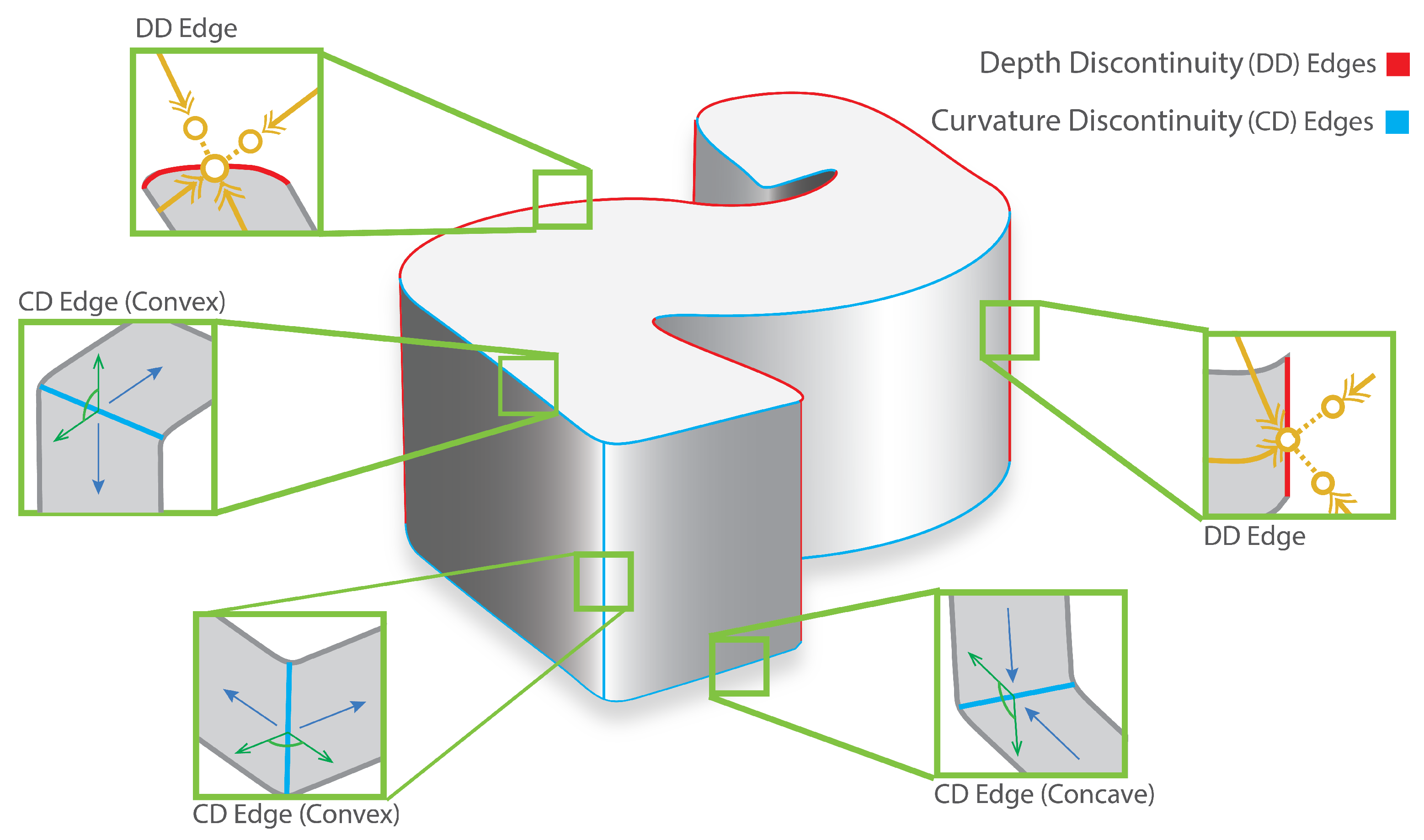
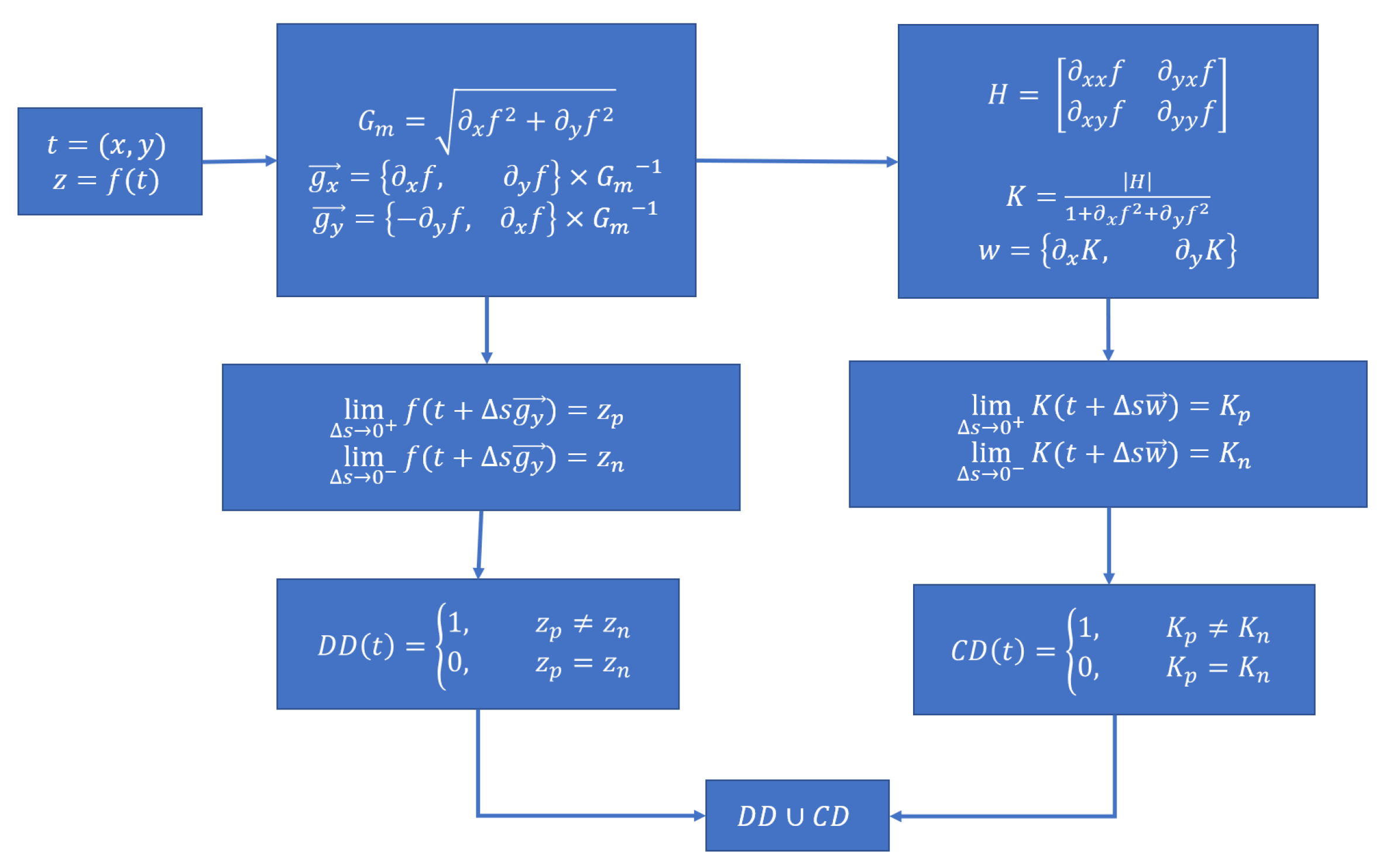
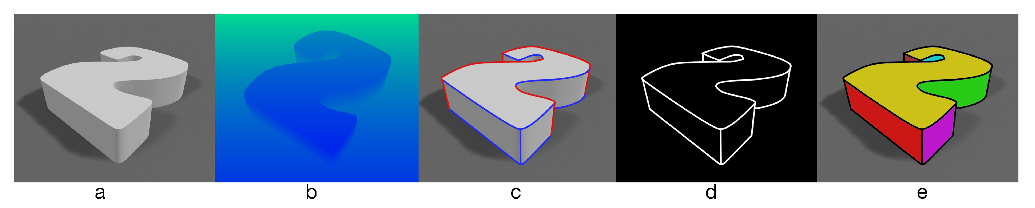
3.1. Isolating Depth Discontinuity Edges

Figure 2 presents the first-principles-based procedures needed to isolate Depth Discontinuity (DD) edges. As noted, a Depth Discontinuity (DD) edge is represented by regions of discontinuity about all directions surrounding a point of interest with the exception of the direction tangential to the interceding boundary separating foreground and background elements. To isolate these regions, we first calculate the gradient f , which results in the vector field F that is oriented in the direction of maximum ascent. Thus, the gradient vector along a DD edge, denoted as G x , lies perpendicular to said edge. From these gradients, we calculate the gradient magnitudes, G M , and further produce the normalized gradient vector g x and the associated orthonormal basis vector g y . Specifically, the g x and g y vectors lay perpendicular and tangential, respectfully, to the underlying depth discontinuity edge. Thus, DD edges are isolated by computing the limit of the depth map f ( x , y ) along the perpendicular vector g x in both the positive and negative directions. Given any discrepancies along said path suggests a discontinuity within the depth map and is therefore associated with a DD edge.

3.2. Isolating Curvature Discontinuity Edges

In addition to depth discontinuity edges, Figure 2 also presents a set of first-principles-based procedures needed to isolate curvature discontinuity (CD) edges to complete the surface segmentation process. To begin, we employ the principle curvature which indicates the direction of maximum slope of a surface and is defined as the derivative of the unit tangent vector to the arc length at that particular point. Thus, the curvature is dependent on regions where the second derivative f ( x , y ) exists within the surface. As mentioned in Section 3, CD edges can be further classified by their convex or concave features. These features are correlated with the direction in which the surface deviates away from the normal plane at the point of interest. As a result, given the Hessian H of the surface presented by the depth map z, the curvature at a point is associated with the definiteness of the Hessian. Thus, given the eigenvalues < λ 1 , λ 2 > = e i g ( H ) : a concave edge is associated with a positive semi-definite Hessian, or by the condition λ 1 0 and λ 2 0 while a convex edge is associated with a negative semi-definite Hessian, λ 1 0 and λ 2 0 . Both values assume λ 1 λ 2 = 0 . Table 1 reviews the relationship between eigenvalues of the Hessian and the type of local curvatures; we ignore elements such as saddle points and planes that do not correspond with the desired curvatures. To isolate the CD edges, we first quantify the curvatures K by calculating the Gaussian curvature across the surface z. Regions of locally maximum curvatures are then located by applying the gradient operator K and selecting regions of high gradient in the curvature of the surface as illustrated in Figure 2. In addition, the concavity of the surface is further identified by determining the definiteness of the Hessian at these points of interest. We capture this information on a binary surface of similar dimensions as our initial surface z.

3.3. Generating Closed Contours

Given the binary depth discontinuity map, D D x , y , and curvature discontinuity map, C D x , y , that both identify the depth and curvature discontinuity edges within the scene, a final union operator is applied to merge these element. This results in raster map of all closed contours M x , y . This is a 2D binary representation of the sets of points that are associated with all closed contour identified in the scene; this process is illustrated Figure 3. As mentioned earlier at the beginning of this section, we then seek to convert these closed-contours embedded in 2D space, M ( x , y ) into a set of 1-dimensional vectors D i such that D i D , where D is the set of all closed contours and D i is a single-dimensional list of all points associated with the contour indexed at ‘i’. We employ a boundary following method defined by Suzuki and Be [22] to convert the rastered contour map M to a set of contours D, with each D i D representing the boundaries of a surface segment within the scene. We briefly review the details of this approach in Section 4.2.
Given the basic approach described above, Figure 4 demonstrates the segmentation quality when applied to synthetic and real-world datasets. The results indicate that noise and other external perturbations, when not accounted for, can severely impact segmentation performance. Correspondingly, it is expected that all real-world capturing instruments are susceptible to such noise and other negative influences. Thus, we continue by proposing a set of robustification measures that are applied to attenuate noise and other adverse artifacts that can quickly undermine surface segmentation performance.

3.4. Robustification of Approach

While the surface segmentation approach presented above may perform well on synthetic scenes, applying such an algorithm on real-world data may produce poor segmentation results. This is demonstrated in Figure 4 and Figure 5 which contrast the difference between directly applying a naive surface segmentation approach versus utilizing robustification measures to mitigate unwanted artifacts. These artifacts are a result of the measurement noise and other negative perturbations that may hinder the algorithm’s performance. Notably, noise resulting from object textures, lighting conditions, pixel dropout, signaling interference, and countless other external ailments is inherent to any image-capturing procedure and may introduce volatility that may undermine the segmentation process. In addition to noise, modern depth sensors utilize a technique called "Time-of-Flight", whereby an infrared projector is used to illuminate a scene while a light sensor collects the reflecting photons and measures the round-trip-time taken to interact with the scene and return to the sensor. Because of the physical offset between the floodlight projector and depth sensor, a depth frame may be subjected to a parallax effect whereby the projected regions that are not visible from the depth sensor’s imaging frustum are presented as a shadow of obstructed pixels in the depth frame perspective. These shadowed pixels are called non-depth-return pixels (NDP) and are routinely set to zero, infinity, or NaN to distinguish from valid pixel values across the scene. Thus, this section deals with strengthening the approach defined in Section 3 against this interference to maintain high-quality real-time segmentation regardless of the scene, camera, or lighting conditions.

3.4.1. Depth Frame Noise Filtering

According to Sweeney et al. [23], frames captured by a depth camera are subjected to Gaussian noise and other systematic biases such as range noise, whereby the variance in depth values across time is impacted by pixel distance. We sought to minimize these inconsistencies by introducing a set of filtering techniques before the segmentation process is performed on a frame. To begin, we apply a Wiener filter, as shown in (2), to individual frames to remove any zero-mean Gaussian noise while preserving the topological structures underlying edges and faces. This is achieved by applying a low-pass filter in which the gain is inversely correlated to the variance of a target neighborhood. During this procedure, non-return-depth pixels (NDP) may disproportionately impact statistical values and are therefore carefully omitted from all filtering operations. Thus, regions with a high variance of in-depth values, such as edges, are preserved while regions of low variance, such as planes, are filtered more aggressively. Figure 5 presents the results of our surface segmentation output with and without a Wiener filter applied.
Wiener Filter : G ( r , c ) = μ + σ l σ l + σ g [ f ( r , c ) μ ]
Given a depth frame with marginal noise, derivative operators may greatly exacerbate the noise profile within the frame, thereby undermining the contouring operation. Unlike a Gaussian filter or any other low-pass filtering mechanism, a Wiener filter applies a blurring operation relative to the variance in the spectral density within a local area of the image. Hence, regions with high variation in depth values are more likely to represent corners, edges, or more complex patterns within the scene which may require minimum filtering; in this case, regions showcasing high variance spectral density are left untouched. Likewise, regions with little variation in pixel values are likely to represent flat regions whereby significantly more blurring may be applied. For each pixel, a surrounding region is used to sample pixel values to determine the valid pixel count ( α c ), local mean ( μ l ), and local variance ( σ l ) for the targeted pixel ( f ( r , c ) ). Following these calculations, we rely on the variance across the entire frame ( σ g ) as the representative RMS value of the power spectrum; this is obtained by averaging the local variances. To maintain edges and corners while mitigating noise, the filtering coefficient, μ , is imposed at a pixel by a proportionate amount relative to the local versus global variances. Together, all associated values are used to filter the noise within the depth frame while preserving quality depth edges and corners for the Canny edge operation [24].
Beyond the Wiener filtering procedure, gradient operations are applied to the depth image z to isolate desired features necessary for the surface segmentation process. As mentioned, gradient operations may exacerbate noise inherent to the depth input; thus, we rely on a Sobel kernel instead of a generic gradient operator when performing 2D differentiation. The Sobel operator conveniently applies a low-pass filter after a high-pass differential operator, thereby, smoothing any disturbances that may have been amplified by the gradient operation. Figure 5 underscores the benefit of the Sobel procedure versus a non-smoothing gradient. The additional noise that is filtered is critical to acquiring clean edges while suppressing false positives.

3.4.2. Temporal Depth Jitter

Given a video stream captured from a depth camera, some depth pixels tend to oscillate between valid and Non-Depth-Return Pixels (NDP) values. This is especially the case around boundaries separating NDP and non-NDP pixels. We define this phenomenon as temporal depth jitter and attempt to compensate by applying a running average across a set of consecutive frames. Instead of estimating the values for these pixels as proposed below in Section 3.4.3, we attempt to capture the appropriate value presented by the depth camera. Thus, given j consecutive frames featuring correlating elements that indicates continuity within the scene, we average valid pixel values across time while ignoring invalid values as presented in (3). Because the underlying application for our surface segmentation procedure is to perform robot grasps, we considered a computation feasible solution that may sacrifice microseconds of latency for overall accuracy. Thus, in testing, we found that averaging the prior four frames significantly attenuated noise resulting from jitter while also providing additional filtering to frame-level zero-mean Gaussian noise. Additionally, this procedure strengthens edge quality by filtering uncertainty resulting from noise and other structural biases resulting from the depth sensor.
Frame Averaging : I t r i , c i , t = 1 s ( r i , c i ) k = t j t 0 if f k ( r i , c i , k ) = N D P f k ( r i , c i , k ) if f k ( r i , c i , k ) ! = 0

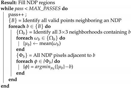
3.4.3. Non-Depth-Return Pixel (NDP) Filling

In addition to zero-mean Gaussian noise and temporal jitter described above, real-world depth images are also subjected to Non-Depth-Return Pixels (NDP) as discussed earlier in this section. While pixel jitter oscillates between valid and invalid values, NDP regions remain invalid across time. Thus, we sought to fill these regions before the segmentation process to maintain consistency across the depth image. This is especially important between foreground and background regions whereby a uniform separation is required to accommodate surface or object manipulation by a robot. Thus, we developed an NDP filling operation to estimate the appropriate values for each depth pixel while also maintaining continuity across the underlying surface. This is especially important when applying any gradient operations across a filled depth image where artifacts may arise from incorrect estimates. This may be the case when estimated values are equal to those of the surrounding environments in which case applying a gradient operator may associate 0 in regions that are not specifically constant. As a result, such a method tends to generate additional artifacts that may undermine the segmentation process. To avoid these artifacts, the the proposed approach attempts to estimate a value that retains the local pixel distribution within the neighborhood of the pixel to be set. To accomplish this, we propose the presented Algorithm 1:
Algorithm 1: The NDP filling process. Each NDP pixel on a valid–invalid boundary is assigned a the mean of its neighborhood.
Robotics 11 00007 i001
For each filling pass, for all NDP pixels, ϕ , neighboring valid pixels are assigned an expected value associated with the means of all eight-connected neighborhoods containing ϕ . While this method does not produce precise estimations of NDP regions, the final solution allows accurate enough contours that closely match the underlying surfaces. The resulting offsets are usually within a margin of error of a few pixels from the ground truth. Such an approach robustifies the depth image from unintended artifacts and uncertainties as a result of NDP regions, while also maintaining real-time performance as a consequence of its simplicity. Figure 6 illustrates the filling process and a filled depth image.

4. Implementation

This section describes the implementation details used to perform real-time surface segmentation on depth maps recorded from real-world data. We apply the approach as described in Section 3 to perform the surface segmentation procedure, and also employ the robustification measures to attenuate noise and other adversarial artifacts stemming from real-world data. We begin by presenting the hardware and software required to perform the actual experiments. This is followed by an overview of the data structures and software architecture used to maintain real-time performance. Finally, we present the entire integration pipeline; from a frame captured from a depth camera to scene segmentation and finally six-DOF surface pose estimation.

4.1. Software Design Architecture

A depth frame is represented by a 2D map of discrete pixel values. In order to perform the surface segmentation operations described in Section 1 while maintaining real-time performance (30+ frames per second (FPS)), we sought to translate the presented continuous algorithm to discrete pixel-wise operations. This section covers software design details and the necessary application structures utilized to maintain real-time performance. We touch on libraries and dependencies used in constructing our application. Data structures and performance algorithms are heavily relied upon to maintain real-time performance. We begin this section by introducing the application pipeline and architecture choices used to maintain faster than real-time performance.

4.1.1. Software and Hardware

During testing, we relied on multiple off-the-shelf RGB-D cameras and online datasets to ensure our algorithm operated robustly across many input devices. We utilized Microsoft’s Azure Kinect RGB-D cameras in addition to an online RGB-D dataset (captured on Microsoft’s Kinect v1 cameras) as inputs to our algorithm. During testing, we rely on the Azure Kinect sensors, wherein the color sensor was configured to operate at 30 frames-per-second with a resolution of 1920 × 1080 while the Depth sensor had been configured to operate at 30 frames-per-second with a resolution of 640 × 576 . The depth sensors maintain an operating range of 0.25 to 3.86 m with a depth uncertainty of less than 0.2% and a random standard deviation error of 17mm. The testing procedure was executed on the Ubuntu 18.08 operating system. This platform consisted of an Intel Core i5 6600K that is clocked at 3.9 GHz across 4 physical cores. For the parallel computing tasks, we relied on an Nvidia GTX 1070 comprising of 1920 CUDA cores clocked at 1683 MHz. Given these specifications, we were able to achieve nearly perfect surface segmentation while also maintaining real-time performance at 30 FPS. On the software side of things, we sought to rely on performant and portable software to maintain cross-platform support. Thus, our algorithm was primarily written in C++ along with a highly parallel procedures written in Nvidia’s CUDA. We also relied on the OpenCV computer vision library which allows us to integrate the more trivial algorithms into our pipeline. This includes Canny Edge Detect to visualize our detected edges, and a contour extraction procedure which is used to separate contours embedded in a 2D frame to a set of 1D vectors defining the contour shape.

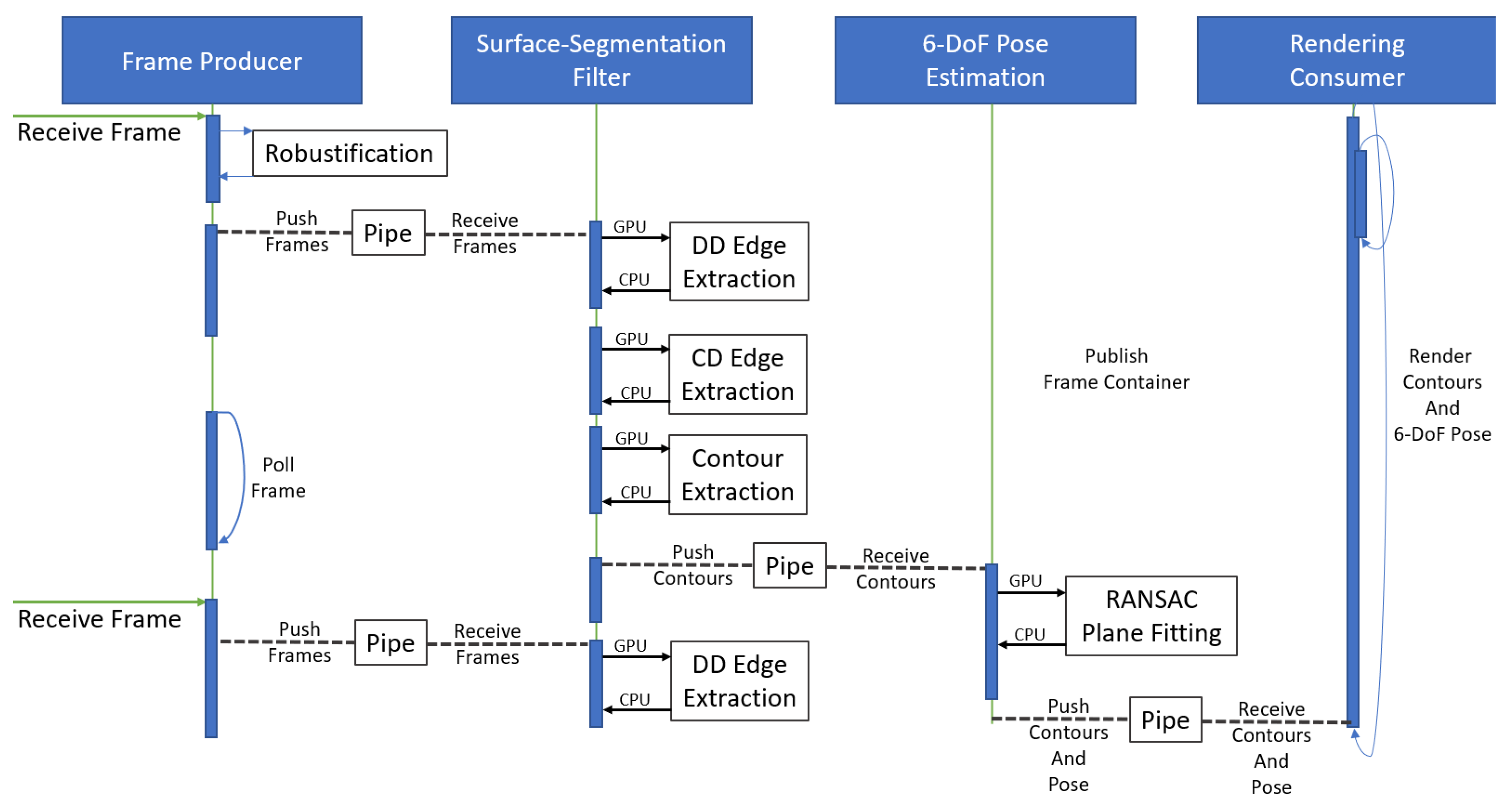
4.1.2. System Architecture

One of the main goals in designing our applications was to allow various strategies to be chained together in such a way as to allow a robot to robustly interact with its environment in real-time. To accomplish this, we rely on a pipeline architecture approach wherein each frame captured from a scene is fed into an algorithm stack and a final rendering policy is presented as an output. The internal group of perception-based algorithms used within the pipeline to accomplish such a task is commonly known as filters. To maintain real-time performance, each filter within a pipeline should accomplish its task within 30 milliseconds, and the entire pass-through time along the pipeline should also not exceed 30 milliseconds. A brief example of a simple filtering pipeline is present in Figure 7 where a pre-processing filter captures and performs filtering on an input before forwarding the resulting data to the next pipeline stage. This process continues until a final consumer stage renders the resulting data to display. For thread safety, a shared double-ended queue implemented as an underlying circular buffer is used to transfer information across pipeline stages. After completing its task, a pipeline filter waits for subsequent data to be provided by the prior filter. Each filter is allocated a set of CPU threads depending on its performance requirements. Thus, our application pipeline can capture RGB-D frames on a FIFO basis, wherein pre-processing filtering is applied as described previously in Section 3.4 before relaying these frames to the Surface Segmentation process. This process further applies a series of lower-level filtering algorithm to remove additional noise and capture object segments within the scene. Because the procedures to perform the surface segmentation algorithm are performed in series, each executable step underlying the algorithm may also be considered a self-contained node that could be assigned its pipeline stage. For instance, the DD edge procedure, and CD edge procedure may have been extracted as an entirely separate node. We decided to keep these procedures in line to maintain design cohesion. Moreover, the application architecture allows algorithms to be executed on any arbitrary device. In this case, the underlying surface-segmentation algorithms utilize the GPU to accelerate performance. Thus, these procedures were written primarily in CUDA, but GLSL or general x86 implementations may also be utilized where possible. The individual stages of our architecture are illustrated in the UML diagram of Figure 8.
The surface-segmentation stage of the pipeline outputs an array of closed contours defined by a list of connected points underlying the contour overall shape. To calculate the six-DOF pose for each contour, a subsequent plane-fitting stage is appended to the pipeline. This stage applies a random sampling consensus operation to each surface segment to estimate its six-DOF pose as described in Section 4.2.4. While beyond the scope of this paper, a final grasp querying stage could also be outfitted to the pipeline whereby individual contours are assessed for potential grasping candidates using their contour information and associated six-DOF pose. Furthermore, in an attempt to maximize performance, highly parallelizable operations are executed on system’s GPU using Nvidia’s CUDA application interface. To summarize, a CPU-based implementation is generally executed in series on the platform processor, which is adept at highly complex branching routines. In contrast, a CUDA-based algorithm is executed on the system’s Graphics Processing Unit (GPU) and is dependent on highly parallel numerical routines. Image processing, for instance, relies on per-pixel mathematical operations to achieve desired results. In this case, each pixel is allocated a particular CUDA thread that performs the actual mathematical operation and stores the desired results to an associated image buffer. As an added performance bonus, during GPU execution, the CPU thread is also left free to perform complex operations. As such, in the case of the surface-segmentation pipeline stage, the Depth Discontinuity operation is initially calculated on the GPU while the CPU prepares for the Curvature Discontinuity algorithm by allocating the necessary resources. At completion, both the GPU and CPU results are merged to create a set of closed contours which is then advanced to the next pipeline stage.

4.2. Software Implementation

Beginning with a depth image received by the Frame-Producer Pipeline node, we present the software implementation details necessary to transform the input data into a set of 1D contours embedded in 2D or 3D environments. This is achieved while mitigating input noise and internal system biases. On completion, we explore localizing potential contact regions and grasping configuration to execute planar grasping on a specified object.

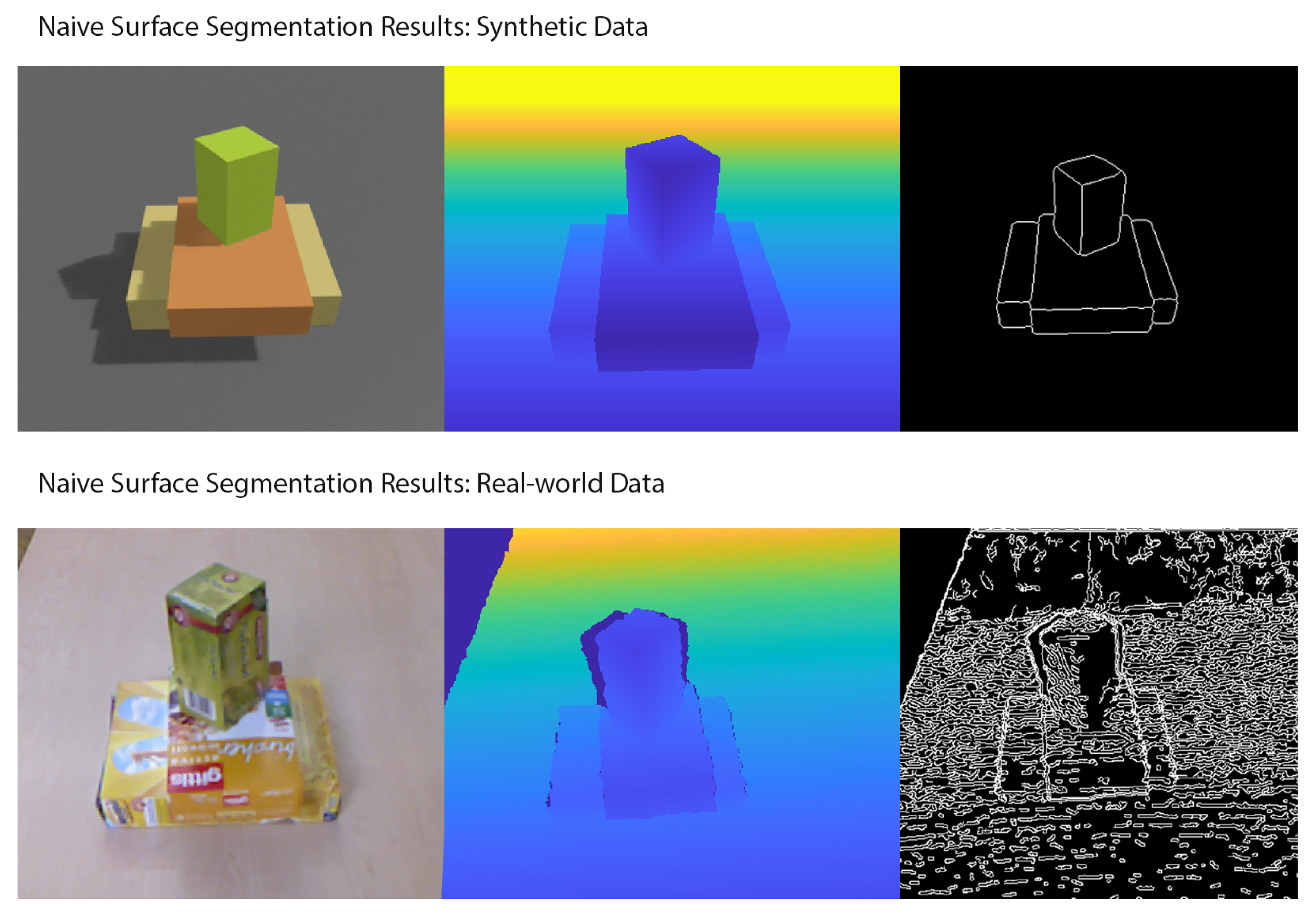
4.2.1. Segmentation Procedure

We sought to limit our research to a video stream comprising solely of 2D depth data visualizing a target scene. We also build upon the premise of [19] which states that stable grasps can be achieved by enacting force closure at contact regions with (i) sharp depth discontinuities or (ii) locally maximal principle curvature in the depth image. As such, we follow the multi-stage approach for achieving real-time surface segmentation as defined in Section 1. We begin with the following data structures:
Depth Frame : d t ( . ) : R 2 R Filtered Depth Frame : d f ( . ) : r o b u s t i f i c a t i o n ( d t ) Filtered Depth Value : z = d f r , c , t
Here, d t denotes a 2D array representing a depth frame at time ( t ), and ( z ) represents the depth value located at the coordinates ( r , c ) at time t . The algorithm begins by applying the robustification measures to the incoming frames to attenuate noise and other negative artifacts. To begin, a running average is performed on the previous 5 incoming frames. As mentioned in Section 3.4.2, this is performed to remove jitter and other range noise associated with any particular frame. This is followed by a heuristic based filling algorithm, established in Section 3.4.3, to close NDP regions with the most likely depth values. Finally, the Wiener filter, as described in Section 3.4.1 is applied to remove zero-mean Gaussian noise. This is all accomplished in the Frame-Producer pipeline subsystem prior to being forwarded to the surface-segmentation subsystem. Subsequently, the filtered frame would finally be routed to the surface-segmentation subsystem where the contouring procedure is applied. To identify DD edges representing surface boundaries within the given scene, we leverage the Canny Edge detect operation to trace regions of high gradient disparity within a single depth frame. This follows the DD extraction approach defined in Section 1 where the horizontal derivatives ( G x ), vertical derivatives ( G y ), and gradient magnitude ( I M ) are used to identify regions of high gradient disparity calculated from (5).
Gradient Vector : I = d f x , d f y T Gradient Magnitude : I M = d f x 2 + d f y 2
The Canny operation considers potential edges as contiguous sets of pixels with locally maximal gradient magnitudes where the associated gradients points in the direction perpendicular to the underlying edge. Thus, it locates region of significant discontinuities within the presented depth image. Though this is able to register edges bounding regions of high gradient changes, it fails to recognize CD edges within the silhouetted regions of the scene. Notwithstanding, the Canny operator is implemented according to the literature [24] to produce edges associated with the scenes’ silhouette. We classify these edges as depth discontinuity (DD) edges and store them in binary 2D array called D D f r a m e .
While a D D f r a m e is being processed, the surface-segmentation subsystem also begins to isolate internal CD edges. As mentioned in Section 3, curvature discontinuity edges are highly correlated with significant change in the curvature of the depth frame. Thus, we establish a series of first principles presented in (6) to isolate these CD edges:
Gradient Direction : I θ = tan 1 I d y / I d x CD * Edges : I C D = I θ x , I θ y T
Instead of relying on the Hessian H as presented in Section 3, we rely on the gradient of the angular offsets within the vector field F. This allows us to forego complex mathematical operations such as calculating the determinant of the Hessian, for a more simple approach of calculating differences in angles. As described in Section 3, the definiteness of the Hessian matrix is still relied upon to determine weather the underlying curvature is convex or concave while the magnitude of the angular values are use to determine the curvature. As a result, we are able to determine CD edges by isolating regions of significant change in the curvature of the depth image. Similar to DD edge, this is accomplished by performing a Canny edge detect operation on the magnitude of the curvature values. The isolated CD edges are stored in a binary 2D array, labeled C D f r a m e , with positive values representing regions of locally maximum curvatures in the depth map.

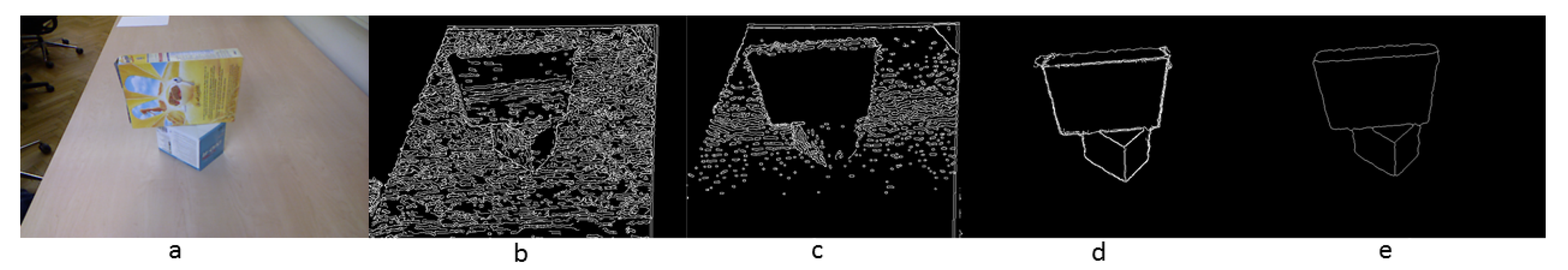
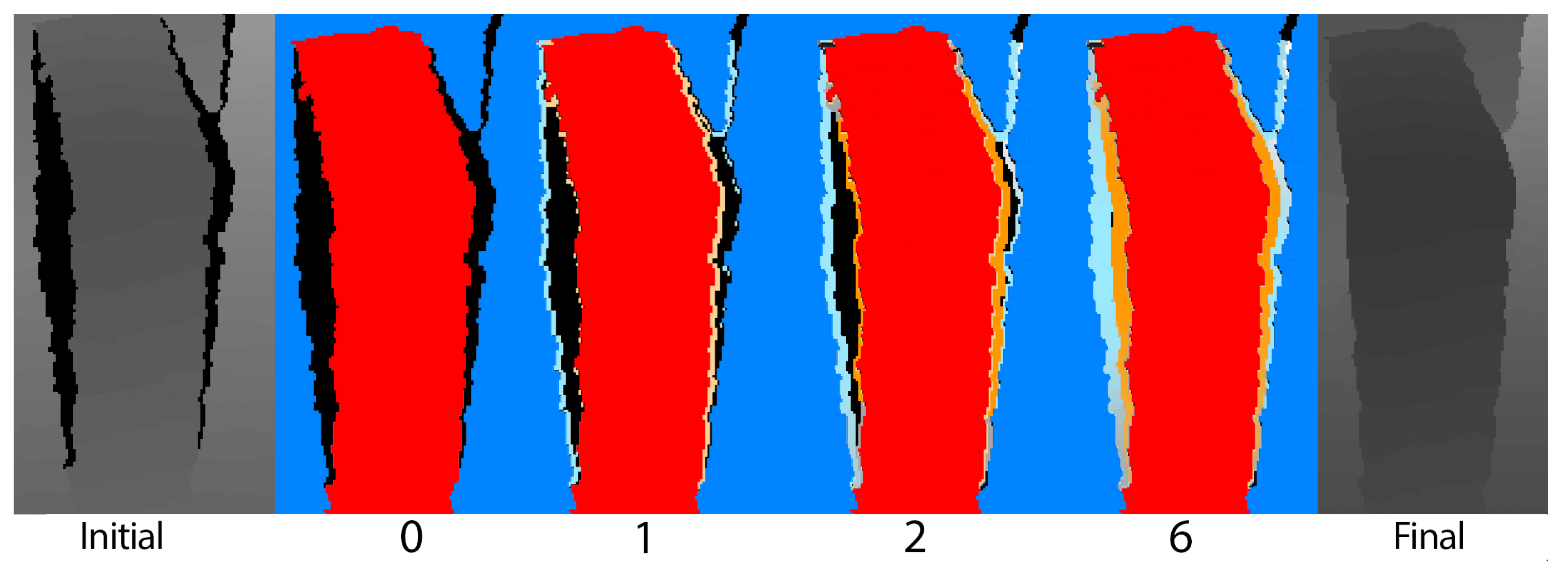
4.2.2. Contour Smoothing

As a result of these operations, we are left with a DD and CD image corresponding to depth discontinuity coordinate locations ( I D D ( . ) : R 2 ) and curvature discontinuity coordinate locations ( I C D ( . ) : R 2 ). Following these procedures, a union operator is applied to established the closed contour regions within the scene. This is followed by an edge smoothing operation performed by a morphological band-pass filter. To accomplish this we perform the following morphological steps:
Step 1. 
A morphological opening operation is employed to obtain the background image, f 01 , from the binarized contours, I c n t r s . The structuring element used in the opening operation, B 1 , is designed to be larger than the high-frequency features that are desired filtered. The concatenated operator is:
f 01 = I c n t r s * B 1 = ( I c n t r s * B 1 ) B 1
where ∘ represents a morphological opening operation encompassing an erosion operation ⊖ and expansion expansion operation, ⊕. This operation expands the bounds width of the contour edges while maintaining the overall form. High-frequency features and noisy elements that are smaller than the structuring elements are thereby excluded.
Step 2. 
The morphological opening operation is employed to obtain the image, f 01 , from the binarized test image, I c n t r s * . The structuring element used in the opening operation is B 2 , which is similar to the measured feature in shape, but slightly smaller in size. The concatenated operator is:
f 02 = I c n t r s B 2 = ( I c n t r s * B 2 ) B 2
In this case, the measured feature and the noise, whose size is smaller than the structuring elements, are excluded.
Step 3. 
The results of morphology band-pass filtering applied to the contour, I c n t r s , is obtained via image differential operations, f 01 and f 02 . The operator is:
I c n t r s = f 02 f 01
The resulting binary image removes high-frequency and low-frequency features, such as kinks and sharp corners, within the contour and presents a smooth set of lines to be used for segmenting.
Remnants of kinks and other filtered perturbations may present themselves as short protrusions from an edge after a morphological band pass filter is applied. To remove these artifacts, we follow the pruning algorithms presented by Jang and Chin [25]. Specifically, we rely on a lookup table (LUT), to decipher the appropriate morphological operation to apply given a specific set of structuring elements B as indicated in Figure 9. Relying on these structuring elements, the pruning process essentially follows the morphological steps realized in (10) as follows:
I 1 = I i n { B } I 2 = 1 8 ( I 1 { B } ) I 3 = ( I 2 H ) I i n I 4 = I 1 I 3
The process begins by applying a thinning procedure to ensure that the contours are within the specified width. The results are then convolved with end-point candidates to isolate all endpoints within the image. We then track these endpoints by performing a dilation and union operation. Finally, a union operation is able to isolate all endpoint pixels within the image. This process is applied recursively to isolate and remove all spurs that may occur within the image. The final result is a smooth contour with high-frequency elements and subsequent spurs removed. From the resulting binary image of embedding contours, we are able to isolate individual surfaces from the scene.

4.2.3. Contour Separation

Given the filtered binarized image, I c n t r s , we sought to separate the representative contour-like features into a list of vectors of varying length whose elements are the contiguous points representing a contour. To accomplish this, we rely on OpenCV’s findContour procedure. This routine implements Suzuki et al. [22], Connected Component Labeling (CCL) algorithm which essentially labels pixels within a binary image with the goal of isolating boundary pixels. This is accomplished by defining a set of constraints which may determine whether a pixel is an inner boundary pixel or outer boundary pixel. The algorithm also keeps track of previously isolated boundaries by labeling these regions with numerical indices. In addition, the algorithm also generates hierarchies of elements based on the contour parent contours enclosing child contours. Thus, the algorithm keeps track of hierarchies by maintaining an index of the previously identified inner and outer indices. These values are defaulted to 1 which indicates that the image frame is considered the root contour. Given the necessary parameters, the algorithm identifies the contours within the depth image by performing the following steps:
Step 1. 
Raster search for pixels satisfying inner, or outer border conditions, and store value of previous visited border as current L N B D value.
Step 2. 
Given a border pixel, assign a numerical index N B D and parent index L N B D to the bordering pixel and all pixels along this currently identified border.
Step 3. 
Upon completion, increment N B D and continue raster search from previously identified border pixel; step (1)
The labeling process is not only able to index individual contours within the scene, but can also group contours into parent child hierarchies based on whether a contour lies in the interior of another. This allows us to track groups of contours which may comprise an entire object and offers potential additional application in the surface merging process. The final result is a set of arrays representing a list of coordinates corresponding to the contours within the image. Thus, we are able to extract the individual contours as a vector list of point describing the bounds surrounding a surface segment. This structure, along with the contour hierarchies, is passed further through our pipeline to be used for visualization purposes or for the principle features needed to perform planar grasping.

4.2.4. Identifying 6-DOF Surface Pose

Figure 10 presents a set of six-DOF poses associated with the segmented surfaces. This is achieved by first applying the proposed segmentation procedure to obtain a set of contours { S } . The subsequent stage of the algorithm extracts the six-DOF pose of the surface segment bounded by the selected contour D i , where the six-DOF pose is comprised of the central position of the surface in addition to 3 degrees associated with orientation. Thus, given a camera’s intrinsic parameters K, we are able to project the depth image into a point cloud using the matrix transform P = K 1 [ x , y , z ] T , where x, y, and z are the 2D coordinates and depth values of the 2D depth image. This results in the transformation of our surface into its associated location in 3D camera space. To determine the centroid of the surface in camera space, we first determine the centroid of the associated contour in the 2D depth-image space. This is achieved by averaging all points across a selected contour, c = 1 M j = 1 M D i j , where i is the index of the selected contour for the surface whose six-DOF pose is desired. The 3D camera-space position is determined by directly transforming the previously determined centroid location, C = K 1 [ c x , c y , f ( c x , c y ) ] T . We then attempt to determine the the orientation of the selected surface by means of plane fitting using a Random Sampling Consensus (RANSAC) algorithm. To summarize, we generate a random consensus set, R, of points derived from the 3D camera space and bounded by surface contour D i . We also define k super-sets of randomly sampled sets G R 3 , where each element G j in G is a random set of 3 points derived from 3D camera space bounded by contour D i . To expand, element G j contains 3 non-collinear points defining a plane. Thus, given k iterations where j identifies the iteration from 1 to k, a plane G j G is selected and the distances d i s t j is define between each point in the consensus set, R, and the iterated plane G j . Thus the plane G α that best fits the surface segment D i is determined by maximizing the formula m a x ( d i s t j < T H R E S H ) , where T H R E S H is the maximum allowable distance from the points to the plane. Thus, the best fitting plane, G α , is selected and its normal axis A n o r m a l or A r o l l further used to identify the pitch and yaw axis of the surface. The yaw axis is obtained by performing a cross product between the calculated normal axis and the general up axis, A y a w = A r o l l × Z . The pitch axis is then determined by the cross product between the surface normal and the previously determined yaw axis A p i t c h = A r o l l × Z . As a result of these operations, the final six-DOF pose of the surface can be represented as [ C x , C y , C z , A p i t c h , A y a w , A r o l l ] . We note here that, given a camera’s extrinsic parameters, these parameters could be trivially transformed to world orientations to aid in robot manipulation.

5. Results

This section presents the image segmentation algorithm applied to multiple imaging sources. Specifically, the OSD dataset is utilized to contrast application performance against Jabalameli and Behal [19]. (Object Segmentation Dataset (OSD) has been collected by researchers in Vienna University of Technology for the purpose of segmenting unknown objects in RGBD images. This dataset consists of 111 manually annotated RGBD images representing table-top isolated objects, stacked objects, and occluded scenes. Diverse kinds of objects in terms of size and shape are included in OSD and these objects are boxes, cups, bowls.) Furthermore, the segmentation procedure is applied to various scenes streamed through Microsoft’s Kinect Depth Camera to showcase the improved segmentation performance on a relatively modern RGB-D capture device. To review, for testing purposes, the algorithm has been applied on a variety of scenes, from basic single object scenes to, highly cluttered scenes filled with variously shaped objects that have not been previously identified. These scenes have been selected to present objects of diverse shapes, sizes, and poses. Performance metrics, such as segmentation accuracy, segmentation run-times, accuracy relative to the number of objects within a scene, and run-time length relative to the number of objects within a particular scene are presented. To elaborate, segmentation accuracy corresponds to the total number of positive surface segments identified within a scene with the true number of surfaces that are present. Likewise, segmentation run-time, represents the total time taken between receiving a single frame of a particular scene and the time presented after the segmentation procedure has been completed. Both accuracy and segmentation run-time performance are also assessed against the number of objects within a given scene. Finally, we conclude with a qualitative results to emphasize the surface-segmentation quality across numerous test scenes of varying levels of clutter. As for the evaluation metrics, the authors aimed to identify groups of surface patches that possibly belong to the same object (perceptual grouping) and categorized the collected scenes into different levels of complexity. For evaluation purposes, eight images were chosen from the OSD with different complexity levels and all the reachable edges for the existing objects were manually marked and considered as graspable edges. If each graspable edge is detected along with correct features, it is counted as a detected edge. In addition, a surface segment is determined graspable if it provides at least one planar force-closure grasp in the camera view and is counted toward the available ground truth surface. In a similar way, graspable ground truth object, and detected object are specified. In this terminology an object is graspable, if there exists at least one feasible grasp configuration compatible with the proposed framework. In a similar way, we consider an object as detected, if the algorithm provides at least one 6D grasp configuration.

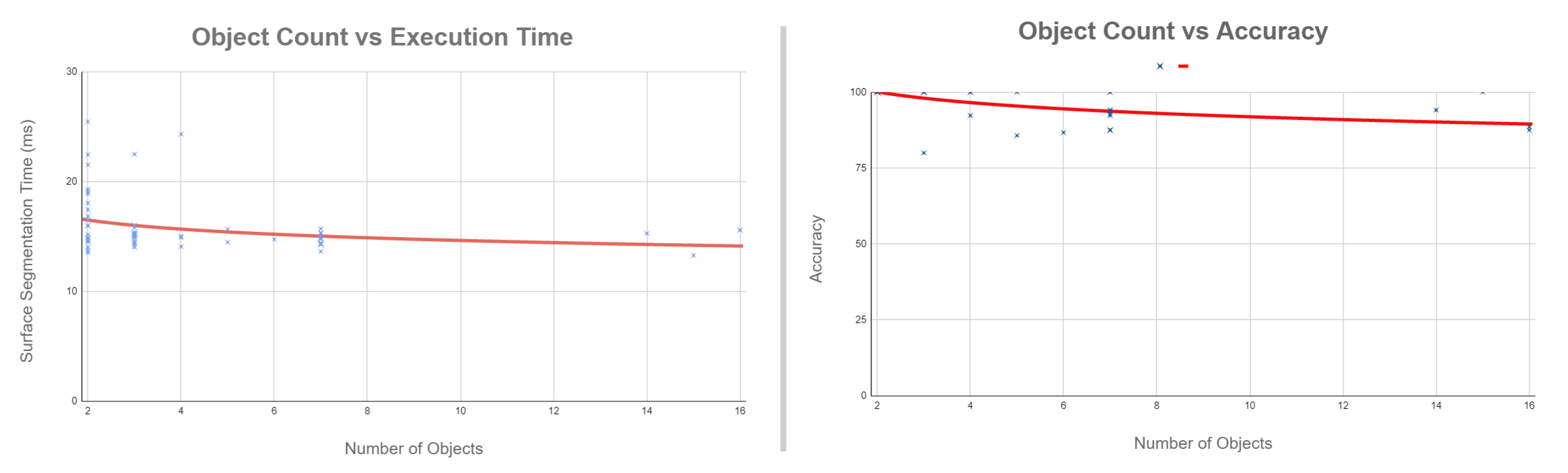
5.1. Performance Comparison

This section scrutinizes the segmentation performance as compared with the results presented in [19]. Because the primary source of comparison is the OSD dataset, the section is primarily focused on static images. As such, the principle objective of this section involves isolating all surface segments within a particular scene and labeling the presented edges as either graspable or non-graspable. It is noted that graspable edges satisfy the convexity test as described in Section 3. To compare our results with [19], we select scenes that are referenced in that research. A select set of these scenes is presented in Figure 11. Scenes are chosen to represent a diverse set of objects and scenarios to challenge even the most state-of-the-art segmenting procedure.
Ground truth data presented by Jabalameli and Behal [19] have been used as the primary mean of comparison. Ref. [19] defines a graspable surface segment as an edge that provides at least one force-closure grasp in the camera view. Thus, it is possible to utilize the isolated closed contours, as discussed in Section 3, by bounding the surface segments to distinguish graspability. This is achieved by simply correlating closed contour convexity (as discussed previously in Section 3.2) to graspability. Thus, a direct comparison could be invoked between [19] and the presented work, including graspable edge classification. Table 2 contrasts the quality of the proposed algorithm against the results presented in [19]. Comparing the presented results underscores the significant gains that the proposed surface segmentation approach has over the prior implementation.
Our review of the data shown in Table 2 showcases not only the significant gains in the amount of positively identified surface segments, the proposed approach also betters the approach in [19] by successfully labeling edges according to graspability. Moreover, it is shown that 99% of all edges across the chosen scenes are positively identified as graspable or non-graspable. Furthermore, the surface identification results showcases near perfect scores across the chosen scenes. Likewise, object identification, which deals with identifying all surfaces for a particular objects, presents near perfect results for the chosen scenes. In comparing run-time performance, the presented algorithm averaged 15.6 milliseconds from the time take to receive a frame to an associated output. In contrast, Ref. [19] notes that the required time needed to proposed edge detection procedure averages approximately 281 milliseconds. These results underscore significant gains achieved by adopting the proposed robustification measures coupled with highly parallel software architecture needed to maintain peak computing performance.

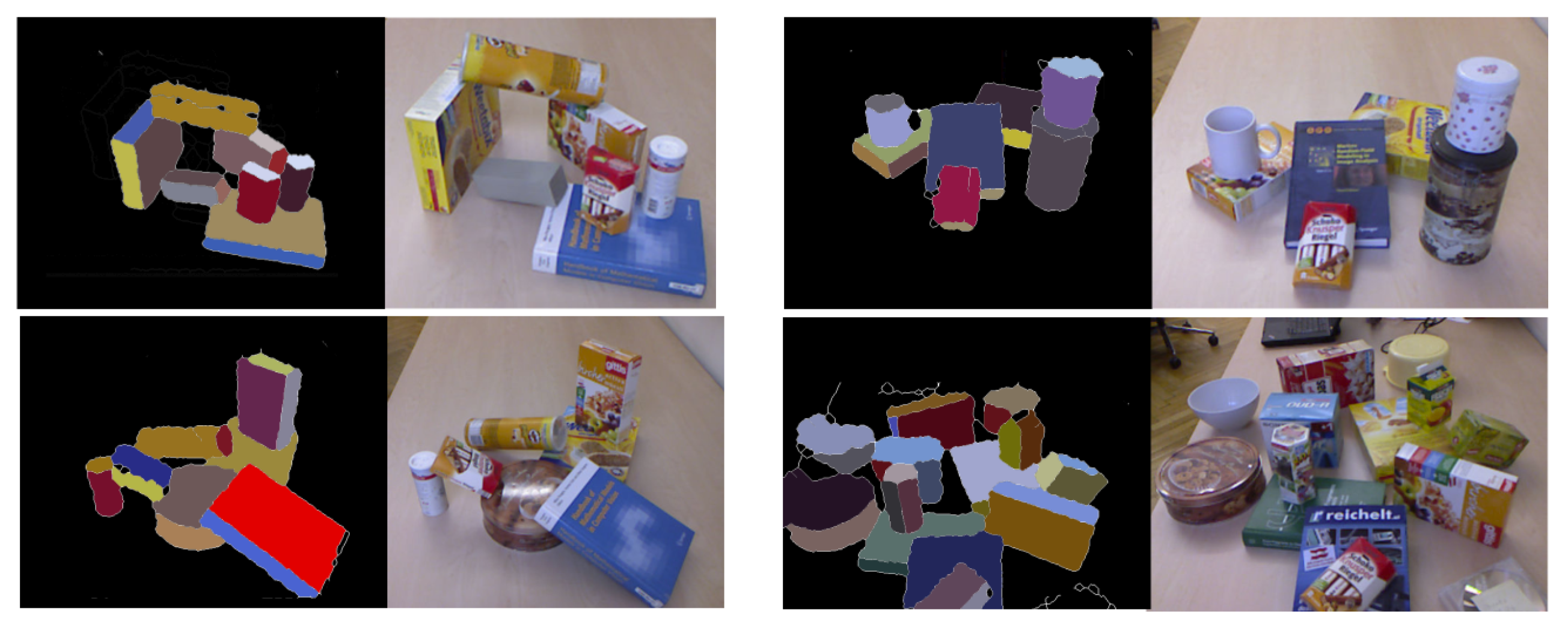
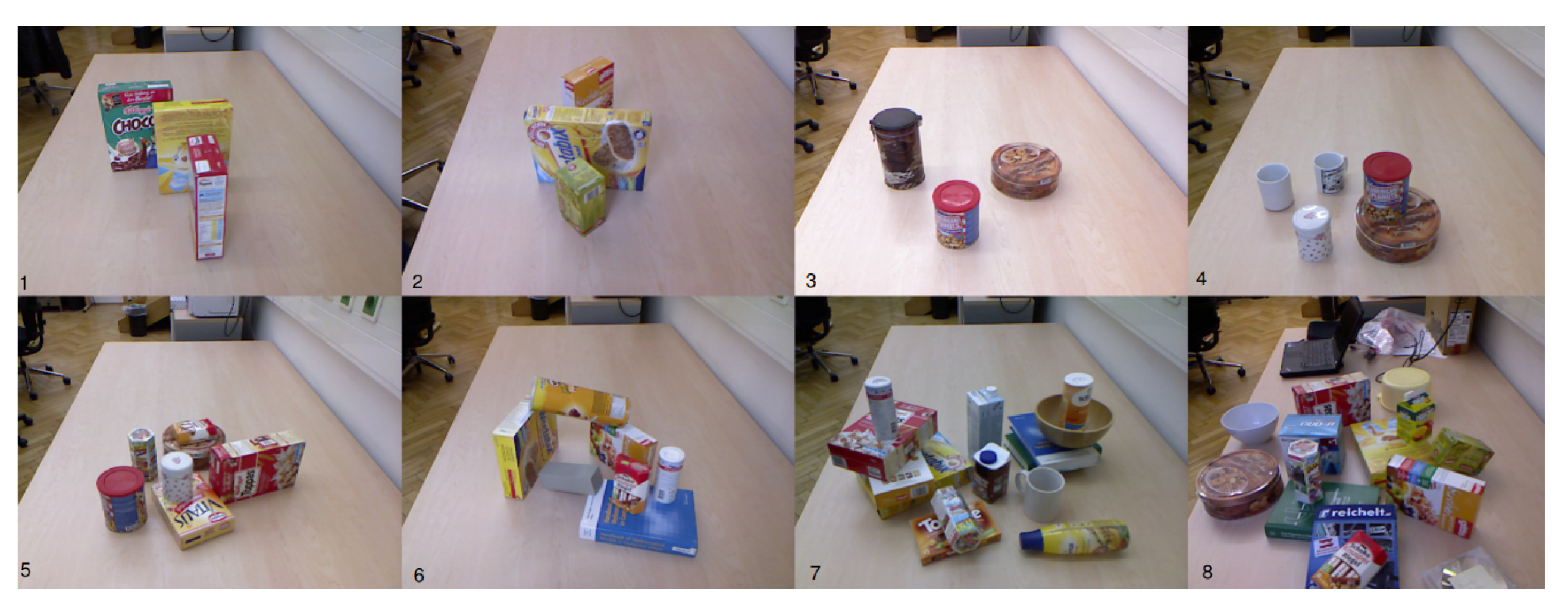
5.2. OSD Dataset Performance

To better understand the overall performance, the framework was executed across the entire OSD dataset. During this test, the proposed framework achieved an average accuracy of 91.51%. In addition, the average performance for each part of the framework has been presented in Table 3. Notably, the approach averages 15.9 ms to segment an entire image. The run-time standard deviation was recorded at 2.6 ms. Given these measurements, we consider the application run-time to be practically invariant to the number of objects within a particular scene. Additionally, the six-DOF surface pose estimation required an additional 1.2 milliseconds on average to compute per selected surface segment. Thus, the average run-time across the entire pipeline is approximately 16.8 milliseconds. The presented time is inclusive of additional overhead required to manage system resources such as CPU-GPU inter-process communication, and general purpose memory management and system routines.
Figure 12 presents a graph comparing process run-time against total objects within a particular scene. According to the figure, it is show that the algorithm is executed in near constant time. Figure 12, also illustrates application accuracy versus the level of clutter within the environment. While the approach maintains great accuracy under less cluttered environments, accuracy falls to 85% for highly cluttered environments.

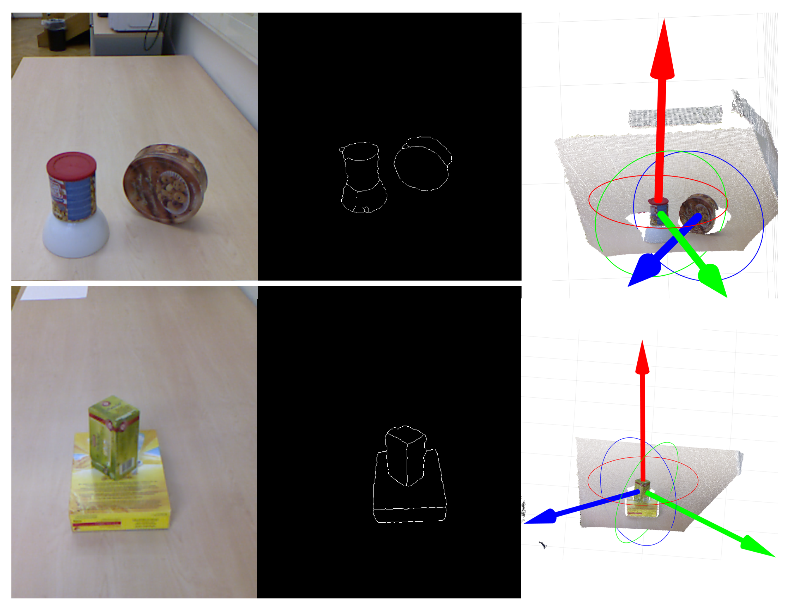
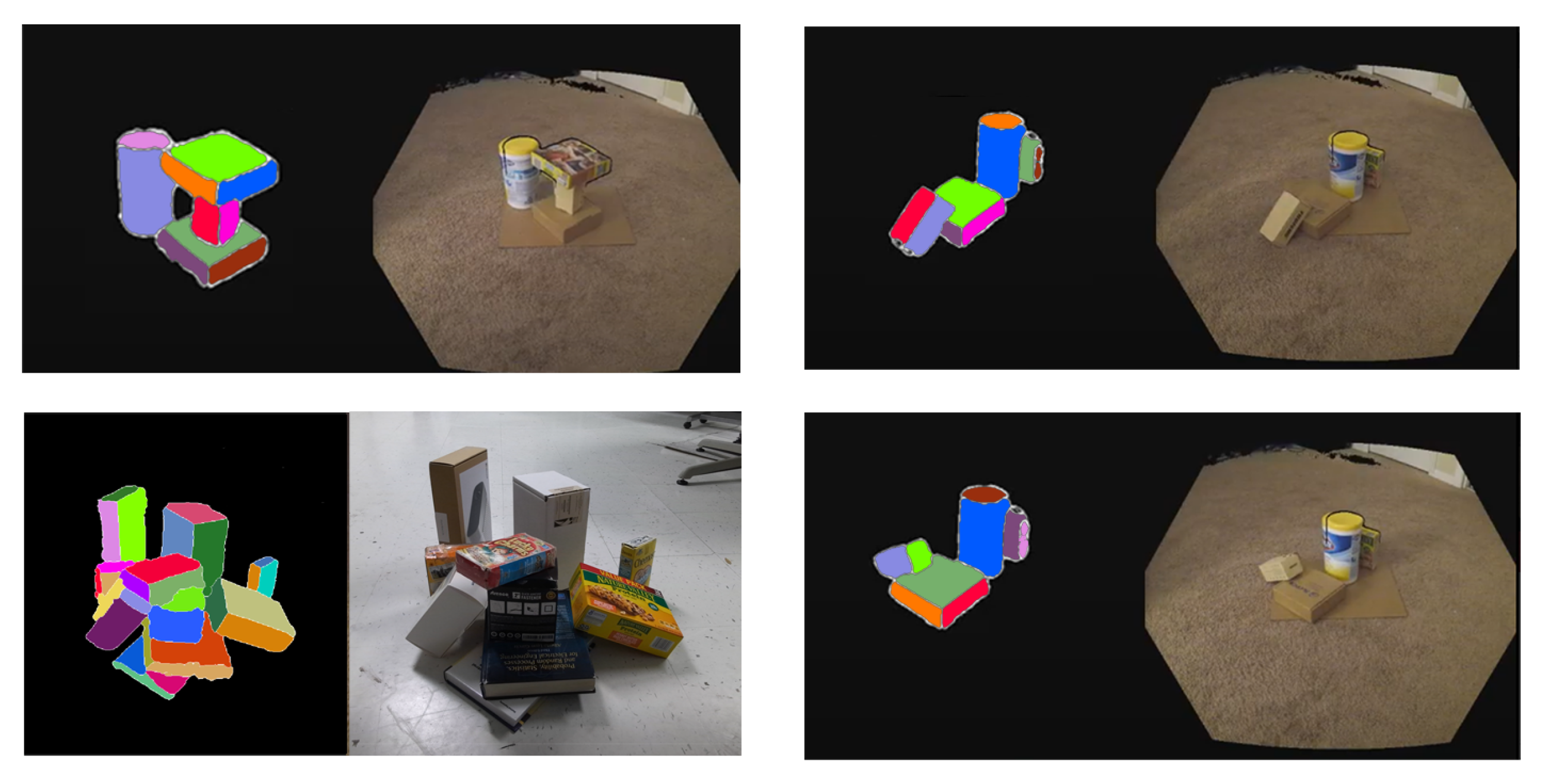
5.3. Qualitative Results

In additional to quantitative results, qualitative results are all presented to showcase segmentation quality across scenes with varying levels of clutter. Figure 13 illustrates these qualitative results across the OSD dataset. The isolated surfaces are coded a distinct color for identification purposes. While the algorithm does not currently apply semantic information when performing the segmentation process, it is apparent that the approach is able to robustly identify individual surfaces of unseen objects within varying environments. Furthermore, the algorithm is able to successfully segment objects differing in shapes—from cylinders, and boxes, to more complex objects like cups and upside-down bowls. It can be observed that the objects are not placed in any particular order but are randomly strewn about, with significant variations in their poses. Nevertheless, the proposed surface segmentation algorithm is able to identify the vast majority of surfaces within the presented scenes, and is able to accurately provide a six-DOF pose to interact with these desired surfaces.
In addition to the OSD datasets, Figure 14 presents the algorithm’s performance on real-time data taken from Microsoft’s Azure Kinect camera. Given a higher quality depth sensor, the presented algorithm is able to better capture individual surfaces across cluttered environments. Even with abnormal poses, the proposed approach maintains real-time performance and high segmentation accuracy as can be seen in the video demonstration provided in [21]. These qualitative results underscore a superior level of robustness as it relates to unseen objects and scenes. Concisely, the proposed algorithm demonstrates an acute level of invariance to rotation, scale, lighting conditions, clutter, and occlusion. Moreover, the proposed approach remains highly effective at segmenting objects even in noisy environments due to the robustification measures that are applied.

6. Discussion

In this section, shortcomings relating to contouring quality and segmentation run-time performance are discussed. To begin, small artifacts resulting from unfiltered noise may present themselves as false-positive contours. Though many of these artifacts are a result of transient noise that may generate fleeting contours, some noise may produce artifacts that may persist across time. Smaller artifacts are trivially removed by filtering contours by size. Consequently, applying such an operation removes contours in the scene after the formation process, resulting in non-uniformly shaped contours which may not encompass the entire surface segment. While most of these persisting artifacts are small enough to be filtered by size, for still frames, larger transient artifacts may persist across frames and are, therefore, more difficult to filter by size or by transient noise. In this case, these contours routinely present themselves as subcontours dividing an actual surface segment. Likewise, false-negative contours may arise as contours may be erroneously merged during the robustification phase. More precisely, while we attempt to utilize a 3 × 3 kernel size for the majority of our convolution and morphological operations, edges that are relatively close together may be merged due to resolution constraints and distance of the surface from the camera. While this may cause a hindrance with lower resolution cameras, the presented approach was able to decipher edges as thin as 5 mm with the camera approximately 1 m away at a resolution of 640 × 578 . A corollary of this would be that, given a high-density depth frame, our proposed approach should be able to exceed the performance presently established in this presentation. In addition to the surface segmentation quality, Figure 12 appears to represent the non-intuitive result that run-time speed is inversely correlated with scene clutter. This discrepancy is a consequence of the contour formation and filter procedures defined in Section 4.2.2 and Section 4.2.3 where larger surface segments require greater execution time to calculate contours details such as size. This results in greater run-times for less cluttered scenes with larger objects.

7. Conclusions

The presented work relies on a first-principles-based approach to segmenting object surfaces within a depth image. This is achieved by identifying and combining discontinuity regions across the depths and curvatures of a depth image. In addition, as shown in the progression in Figure 5, numerous robustification measures are applied to filter noise and other artifacts that are inherent to any real-world data capturing system. Furthermore, given a segment surface, a six-DOF pose is estimated and designated as an end-effector approach vector for object manipulation. By deferring to algorithms presented in [19], a stable grasp can be achieved by performing force and torque closure on the edges of an object’s surface. Thus, a never-before-seen object within an unstructured scene can be manipulated as desired given the outputs of the presented algorithm. Finally, it is demonstrated that the segmentation procedure can achieve a high level of accuracy, even in cluttered environments. Moreover, the segmentation and pose estimation procedures are performed faster than real time and are shown to be more or less invariant to the number of objects in the scene. This allows a robot to optimize strategies through querying grasps and other manipulation techniques by merely altering its perspective. Future research may present a means of merging surfaces to form objects, which may further allow the ability to rank graspable objects based on their relative locations and orientations within a scene. Insofar as the presented software implementation currently stands, this could be implemented as an added pipeline stage to maintain real-time performance.

Author Contributions

Conceptualization, A.B.; Formal analysis, A.J.; Funding acquisition, A.B.; Investigation, Y.R.; Methodology, Y.R. and A.J.; Software, Y.R.; Validation, Y.R.; Visualization, Y.R.; Writing—original draft, Y.R.; Writing—review and editing, A.J. and A.B. All authors have read and agreed to the published version of the manuscript.

Funding

This study was funded in part by NSF grant numbers IIS-1409823 and IIS-1527794, and in part by NIDILRR grant #H133G120275. However, these contents do not necessarily represent the policy of the aforementioned funding agencies, and you should not assume endorsement by the Federal Government.

Institutional Review Board Statement

Not applicable.

Informed Consent Statement

Not applicable.

Data Availability Statement

Publicly available database utilized. Demonstration Video available.

Conflicts of Interest

The authors declare no conflict of interest.

References

  1. Sahbani, S.; El-Khoury, P.B. An overview of 3D object grasp synthesis algorithms. Robot. Auton. Syst. 2012, 60, 326–336. [Google Scholar] [CrossRef] [Green Version]
  2. Bohg, J.; Morales, A.; Asfour, T.; Kragic, D. Data-Driven Grasp Synthesis—A Survey. IEEE Trans. Robot. 2014, 30, 289–309. [Google Scholar] [CrossRef] [Green Version]
  3. Miller, A.; Knoop, S.; Christensen, H.; Allen, P. Automatic Grasp Planning Using Shape Primitives. In Proceedings of the Robotics and Automation, 2003. Proceedings. ICRA’03, IEEE International Conference, Taipei, Taiwan, 14–19 September 2003; Volume 2, pp. 1824–1829. [Google Scholar]
  4. Huebner, K.; Kragic, D. Selection of robot pre-grasps using box-based shape approximation. In Proceedings of the 2008 IEEE/RSJ International Conference on Intelligent Robots and Systems, Nice, France, 22–26 September 2008; pp. 1765–1770. [Google Scholar]
  5. Przybylski, M.; Asfour, T.; Dillmann, R. Planning grasps for robotic hands using a novel object representation based on the medial axis transform. In Proceedings of the 2011 IEEE/RSJ International Conference on Intelligent Robots and Systems, San Francisco, CA, USA, 25–30 September 2011; pp. 1781–1788. [Google Scholar]
  6. Detry, R.; Ek, C.H.; Madry, M.; Kragic, D. Learning a dictionary of prototypical grasp-predicting parts from grasping experience. In Proceedings of the 2013 IEEE International Conference on Robotics and Automation, Karlsruhe, Germany, 6–10 May 2013; pp. 601–608. [Google Scholar] [CrossRef]
  7. Kroemer, O.; Ugur, E.; Oztop, E.; Peters, J. A kernel-based approach to direct action perception. In Proceedings of the 2012 IEEE International Conference on Robotics and Automation, Saint Paul, MI, USA, 14–18 May 2012; pp. 2605–2610. [Google Scholar] [CrossRef]
  8. Kopicki, M.; Detry, R.; Schmidt, F.; Borst, C.; Stolkin, R.; Wyatt, J.L. Learning dexterous grasps that generalise to novel objects by combining hand and contact models. In Proceedings of the 2014 IEEE International Conference on Robotics and Automation (ICRA), Hong Kong, China, 31 May–7 June 2014; pp. 5358–5365. [Google Scholar] [CrossRef] [Green Version]
  9. Saxena, A.; Driemeyer, J.; Ng, A.Y. Robotic grasping of novel objects using vision. Int. J. Robot. Res. 2008, 27, 157–173. [Google Scholar] [CrossRef] [Green Version]
  10. Morrison, D.; Corke, P.; Leitner, J. Closing the Loop for Robotic Grasping: A Real-time, Generative Grasp Synthesis Approach. In Proceedings of the Robotics: Science and Systems (RSS), Pittsburgh, PA, USA, 26–28 June 2018. [Google Scholar]
  11. Liang, H.; Ma, X.; Li, S.; Gorner, M.; Tang, S.; Fang, B.; Sun, F.; Zhang, J. PointNetGPD: Detecting grasp configurations from point sets. In Proceedings of the IEEE International Conference on Robotics and Automation (ICRA), Montreal, QC, Canada, 20–24 May 2019. [Google Scholar]
  12. Mahler, J.; Liang, J.; Niyaz, S.; Laskey, M.; Doan, R.; Liu, X.; Ojea, J.A.; Goldberg, K. Dex-net 2.0: Deep learning to plan robust grasps with synthetic point clouds and analytic grasp metrics. In Proceedings of the Robotics: Science and Systems, Cambridge, MA, USA, 12–16 July 2017. [Google Scholar]
  13. Kappler, D.; Bohg, J.; Schaal, S. Leveraging big data for grasp planning. In Proceedings of the IEEE International Conference on Robotics and Automation (ICRA), Seattle, WA, USA, 26–30 May 2015; pp. 4304–4311. [Google Scholar]
  14. Pinto, L.; Gupta, A. Supersizing self-supervision: Learning to grasp from 50k tries and 700 robot hours. In Proceedings of the 2016 IEEE International Conference on Robotics and Automation (ICRA), Stockholm, Sweden, 16–21 May 2016; pp. 3406–3413. [Google Scholar]
  15. Schmidt, P.; Vahrenkamp, N.; Wachter, M.; Asfour, T. Grasping of unknown objects using deep convolutional neural networks based on depth images. In Proceedings of the IEEE International Conference on Robotics and Automation (ICRA), Brisbane, Australia, 21–25 May 2018; pp. 6831–6838. [Google Scholar]
  16. Veres, M.; Moussa, M.; Taylor, G.W. Modeling grasp motor imagery through deep conditional generative models. IEEE Robot. Autom. Lett. 2017, 2, 757–764. [Google Scholar] [CrossRef] [Green Version]
  17. Mahler, J.; Matl, M.; Satish, V.; Danielczuk, M.; DeRose, B.; McKinley, S.; Goldberg, K. Learning ambidextrous robot grasping policies. Sci. Robot. 2019, 4, 26. [Google Scholar] [CrossRef] [PubMed]
  18. Montaño, A.; Suárez, R. Dexterous Manipulation of Unknown Objects Using Virtual Contact Points. Robotics 2019, 8, 86. [Google Scholar] [CrossRef] [Green Version]
  19. Jabalameli, A.; Behal, A. From Single 2D Depth Image to Gripper 6D Pose Estimation: A Fast and Robust Algorithm for Grabbing Objects in Cluttered Scenes. Robotics 2019, 8, 63. [Google Scholar] [CrossRef] [Green Version]
  20. Nguyen, V. Constructing force-closure grasps. In Proceedings of the 1986 IEEE International Conference on Robotics and Automation, San Francisco, CA, USA, 7–10 April 1986; Volume 3, pp. 1368–1373. [Google Scholar]
  21. Roberts, Y.; Jabalameli, A.; Behal, A. Surface Segmentation Video Demonstration. 2020. Available online: https://youtu.be/2KkEk_INvTM (accessed on 12 September 2021).
  22. Suzuki, S.; Be, K. Topological structural analysis of digitized binary images by border following. Comput. Vision Graph. Image Process. 1985, 30, 32–46. [Google Scholar] [CrossRef]
  23. Sweeney, C.; Izatt, G.; Tedrake, R. A Supervised Approach to Predicting Noise in Depth Images. In Proceedings of the 2019 International Conference on Robotics and Automation (ICRA), Montreal, QC, Canada, 20–24 May 2019; pp. 796–802. [Google Scholar] [CrossRef]
  24. Canny, J. A Computational Approach to Edge Detection. IEEE Trans. Pattern Anal. Mach. Intell. 1986, PAMI-8, 679–698. [Google Scholar] [CrossRef]
  25. Jang, B.K.; Chin, R. Analysis of thinning algorithms using mathematical morphology. IEEE Trans. Pattern Anal. Mach. Intell. 1990, 12, 541–551. [Google Scholar] [CrossRef]
Figure 1. An illustration showcasing Depth Discontinuity (DD) and Curvature Discontinuity (CD) features that are used to isolate surfaces within a scene.
Robotics 11 00007 g001
Figure 2. A flow diagram indicating the logic operations performed on a depth map to obtain DD and CD features necessary in generating surface contours.
Robotics 11 00007 g002
Figure 3. Series of steps relied upon to isolate individual surface segments. (a) Initial Scene (usually depicted by an RGB image). (b) Depth Map in accordance with z = f ( x , y ) . (c) Extracted DD (red) and CD (blue) features as described in section above. (d) Closed contours generated by a union operation of DD and CD maps. (e) Final segmentation process separates the surfaces with respect to their bounding contours. In this case, each contour is represented by a distinct color.
Robotics 11 00007 g003
Figure 4. Naive surface segmentation approach applied to synthetically generated scene (above) contrasted naive results applied to an unfiltered real-world scene (below). (left) RGB capture of the scene. (center) Depth Image. (right) resulting segmentation.
Robotics 11 00007 g004
Figure 5. A series of steps needed to robustify a depth frame against noise. (a) RGB Image. (b) Filtering results without any robustification measures. (c) Results with a Wiener filter applied. (d) Results with Wiener Filter and Sobel Operator. (e) Results with Wiener Filtering, Sobel Operator, and Edge Smoothing.
Robotics 11 00007 g005
Figure 6. NDP filling passes. Left to right: beginning with initial depth image (left), set boundary NDP pixels using the proposed averaging technique until NDP regions are filled (right).
Robotics 11 00007 g006
Figure 7. An example of a pipeline containing multiple filtering stages.
Robotics 11 00007 g007
Figure 8. Overall program architecture use to perform surface segmentation and extract 6-DOF surface pose.
Robotics 11 00007 g008
Figure 9. Set of structuring elements used as Pruning templates to decide whether a pixel should be removed [25].
Robotics 11 00007 g009
Figure 10. Illustration of 6-DOF Surface pose estimation. (Left) Scene. (Center) Contours. (Right) Point Cloud showcasing various surface poses.
Robotics 11 00007 g010
Figure 11. The subset of images presented by [19] during their simulation illustration.
Robotics 11 00007 g011
Figure 12. Left: Number of Surfaces in a scene versus execution time. Execution time is invariant to scene complexity. Right: Accuracy versus number of surfaces within a scene.
Robotics 11 00007 g012
Figure 13. Qualitative surface-segmentation results of cluttered scenes from the OSD dataset. The results presents the case that our proposed algorithm is able to capture surfaces across cluttered scenes.
Robotics 11 00007 g013
Figure 14. Qualitative surface-segmentation results of scenes streamed form Microsoft’s Acure Kinect Camera.
Robotics 11 00007 g014
Table 1. Correlation between the sign of the Eigen values of the Hessian matrix and curvature type.
λ 1 >0=0<0
λ 2 >0ConcaveConcaveSaddle
=0ConcavePlaneConvex
<0SaddleConvexConvex
Table 2. Column comparing the number of Detected objects, surface segments, and edges with Jabalameli and Behal [19]. GT: Ground truth; LC: low clutter; HC: high clutter.
SceneGT. ObjectProposed[19]GT. SurfaceProposed[19]GT. EdgeProposed[19]
1Boxes333666171714
2Boxes333888202017
3Cylinders333665121210
4Cylinders55510109202019
5Mixed - LC66613139282821
6Mixed - LC77713139282822
7Mixed - HC111111242417555342
8Mixed - HC141410222216494733
100.00%92.31% 100.00%77.45% 98.25%77.73%
Table 3. Average performance in milliseconds across individual stages of the segmentation process. Total time includes the sum of all operations in addition to post-processing procedures and system overhead.
NDP FillDD OprWienerSobelCD OprCannyMorphologyValidationTotal Time
0.66 ± 0.00.21 ± 0.02.10 ± 0.30.84 ± 0.00.36 ± 0.30.34 ± 0.34.80 ± 0.51.87 ± 0.215.9 ± 2.6
Publisher’s Note: MDPI stays neutral with regard to jurisdictional claims in published maps and institutional affiliations.

