
Implementation of a Flexible and Lightweight Depth-Based Visual Servoing Solution for Feature Detection and Tracing of Large, Spatially-Varying Manufacturing Workpieces

 and
and 
Abstract
:1. Introduction
2. Methods and Materials
2.1. Selection of Physical Camera and Kinematic Robot
2.2. Selection of Software
2.3. Algorithm Design
2.3.1. Acute Edge Detection
2.3.2. Obtuse Edge Detection
3. Experimental Setup
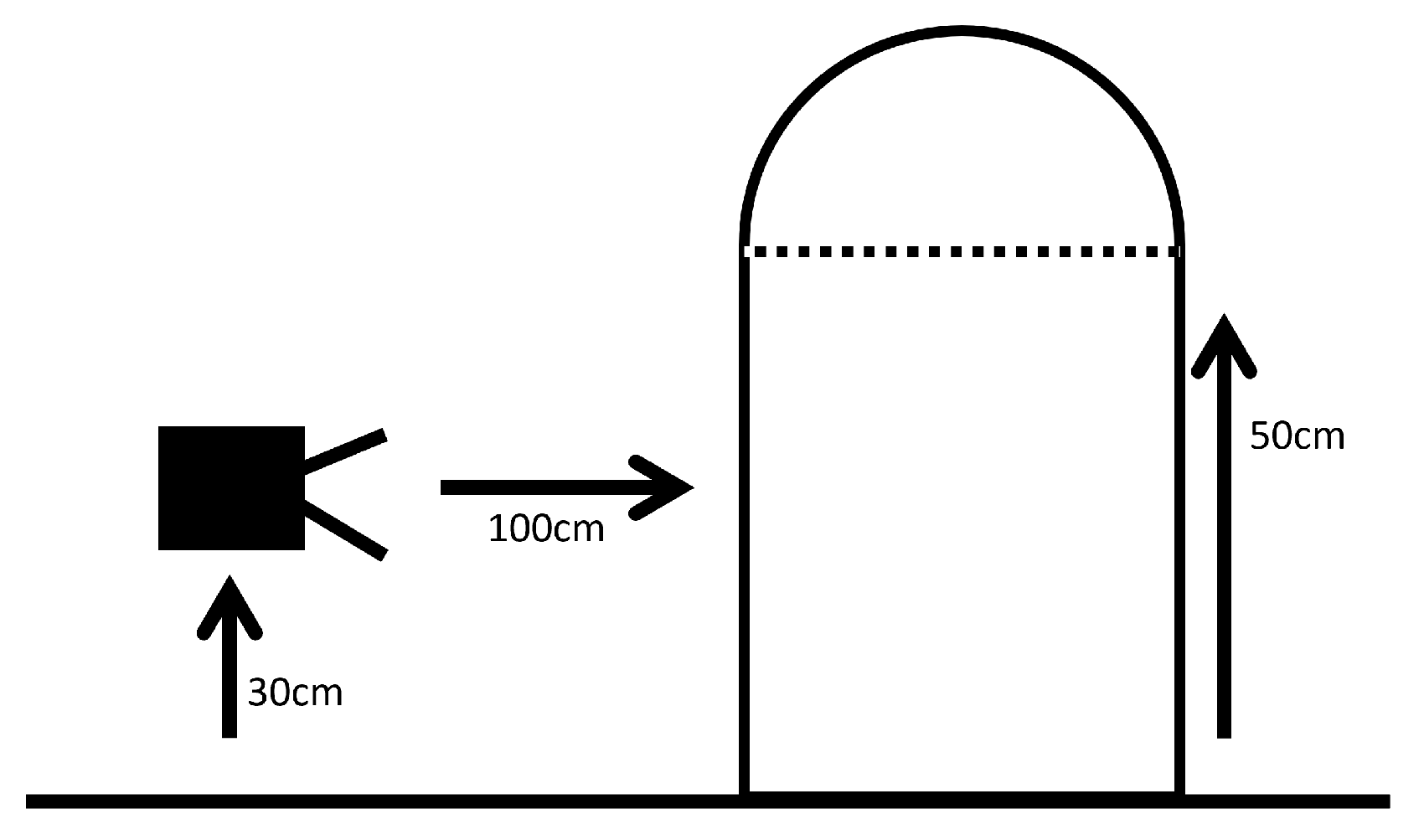
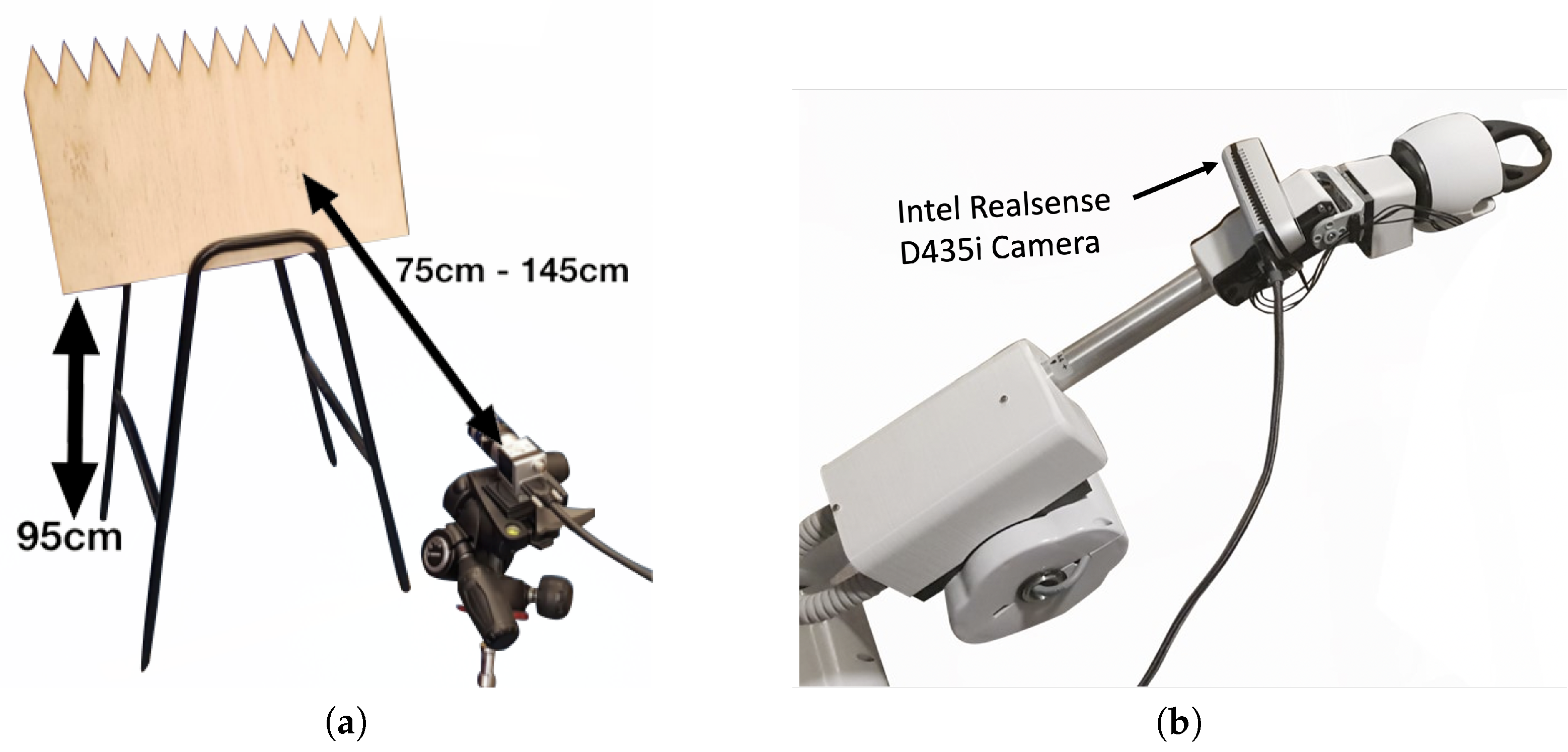
3.1. Environmental Variable Experimentation
3.2. Acute Feature Detection and Tracking
3.3. Obtuse Feature Detection and Tracking
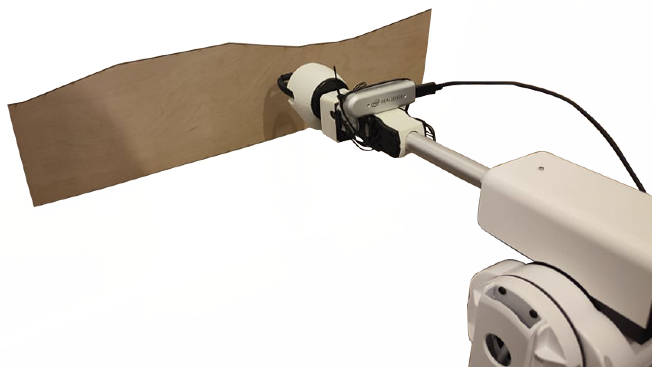
3.4. Physical Detection and Tracing
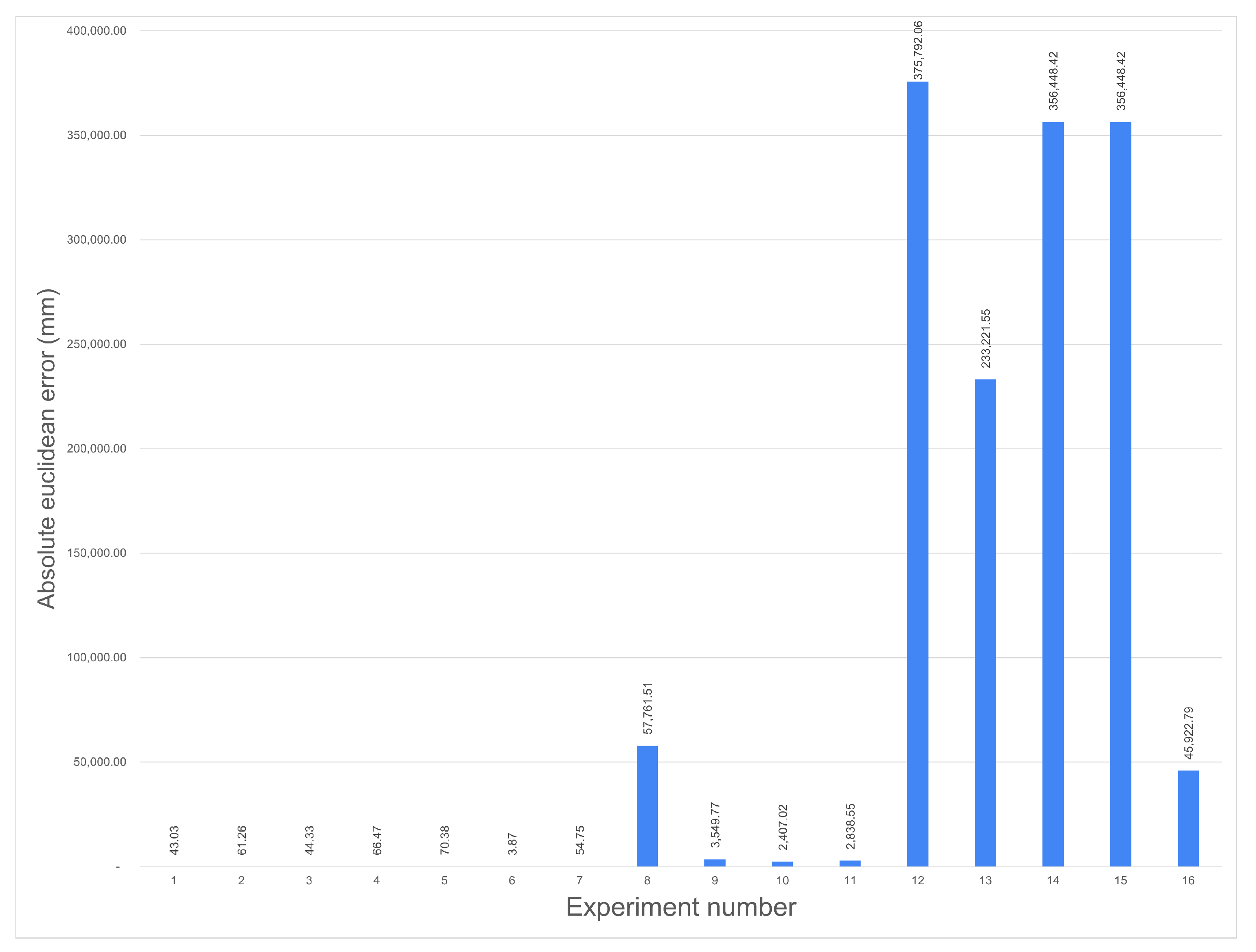
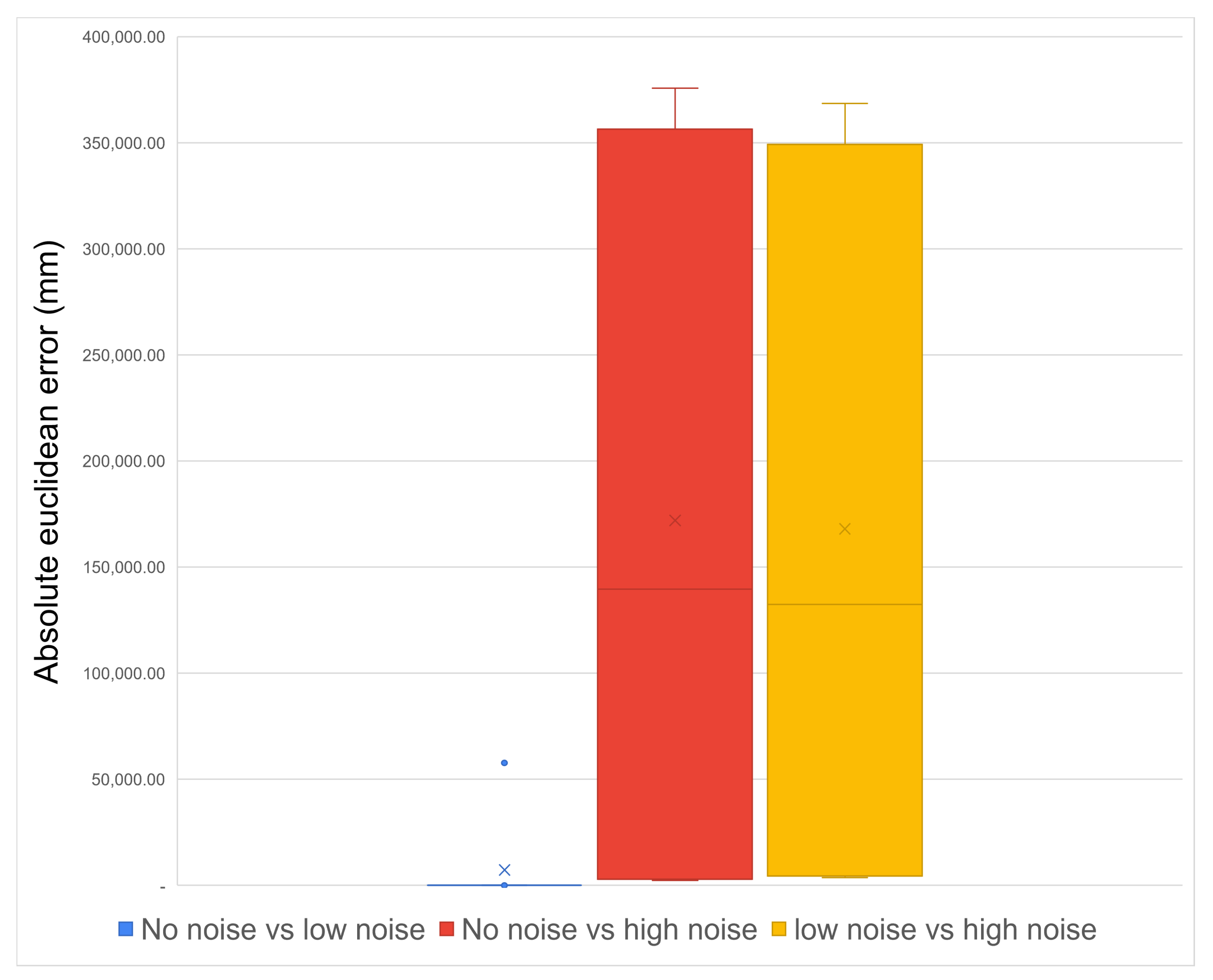
4. Results and Discussion
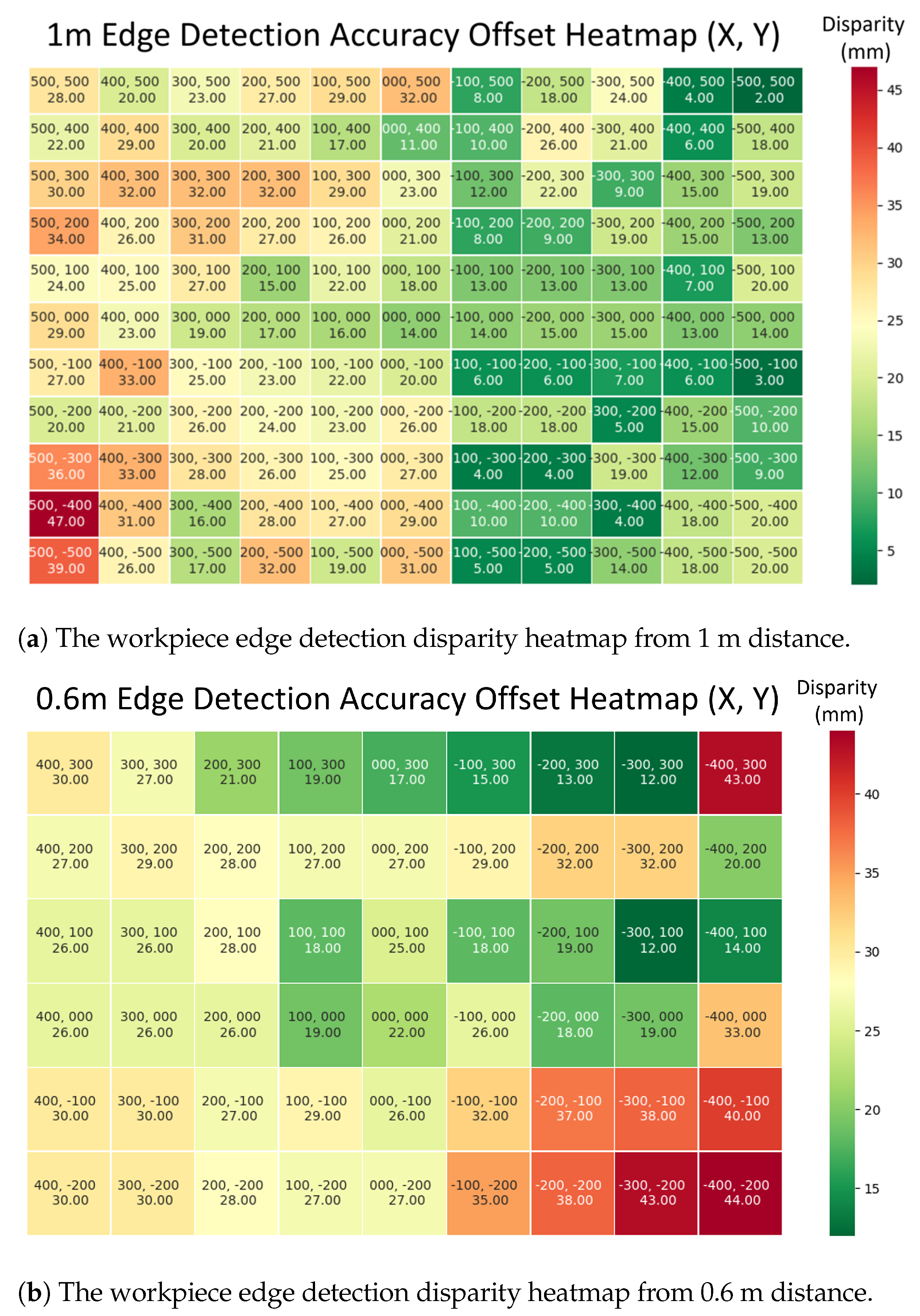
4.1. Identification of Best Environmental Parametres
- While on its own, the aperture had a significant effect on the final image, as expected, as it controlled how much light was let into the lens as well as the lens depth of focus. When combined with lighting, these became the two variables with the strongest interdependencies. This was expected as the two variables complemented each other and directly affected how the other one would affect the image;
- Similarly, the second strongest interdependency was focus and distance. Individually both of these variables had little effect on the final image but combined, they interacted to either create a focused image or one which was entirely out of focus;
- Unsurprisingly, the variable with the smallest impact was the environment’s lighting, due to how the minimal lighting setting selected was not total darkness, but having one of the possible three lights on, producing a value of 478 lux. This was done to consistently provide usable images and not cause anomalies with the other variables.
4.2. Feature Identification and Tracing
4.2.1. Acute Feature Identification and Extraction
4.2.2. Obtuse Feature Identification and Extraction
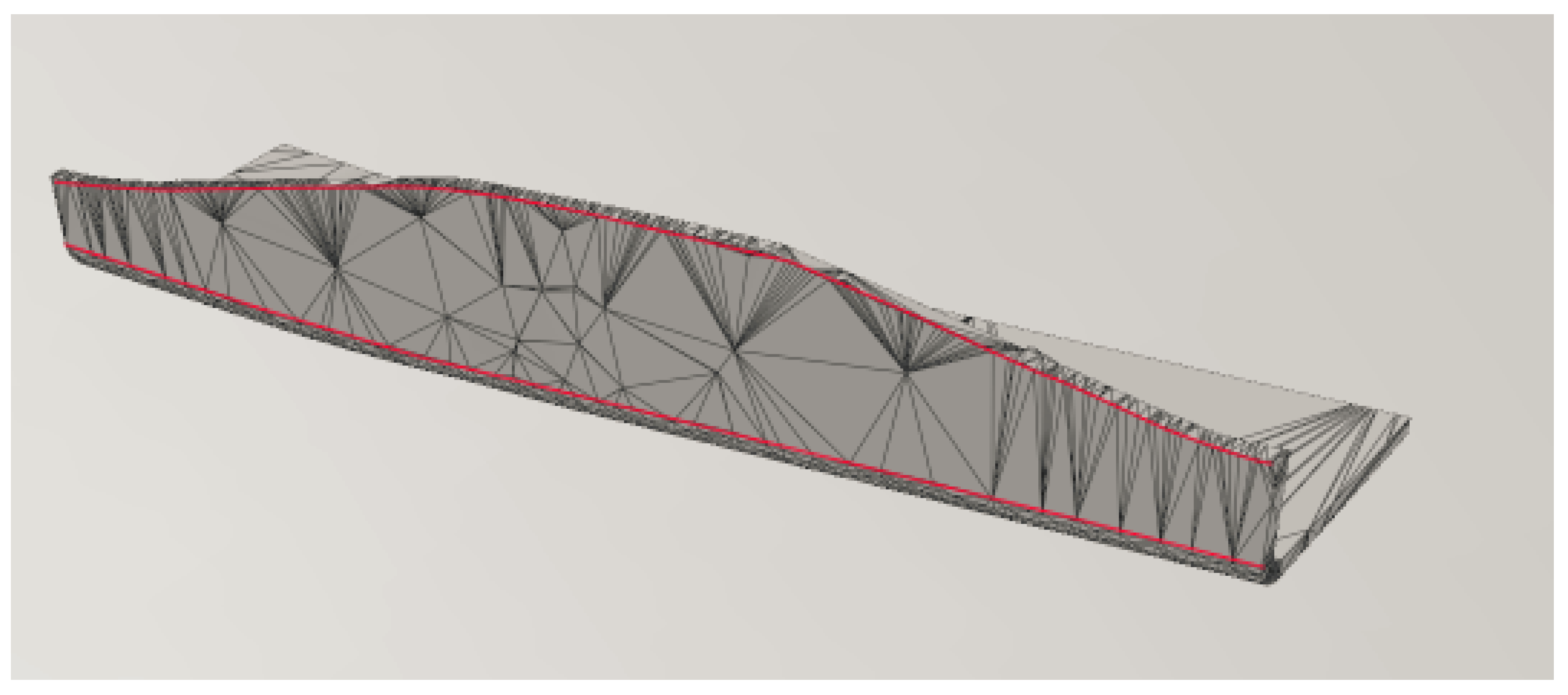
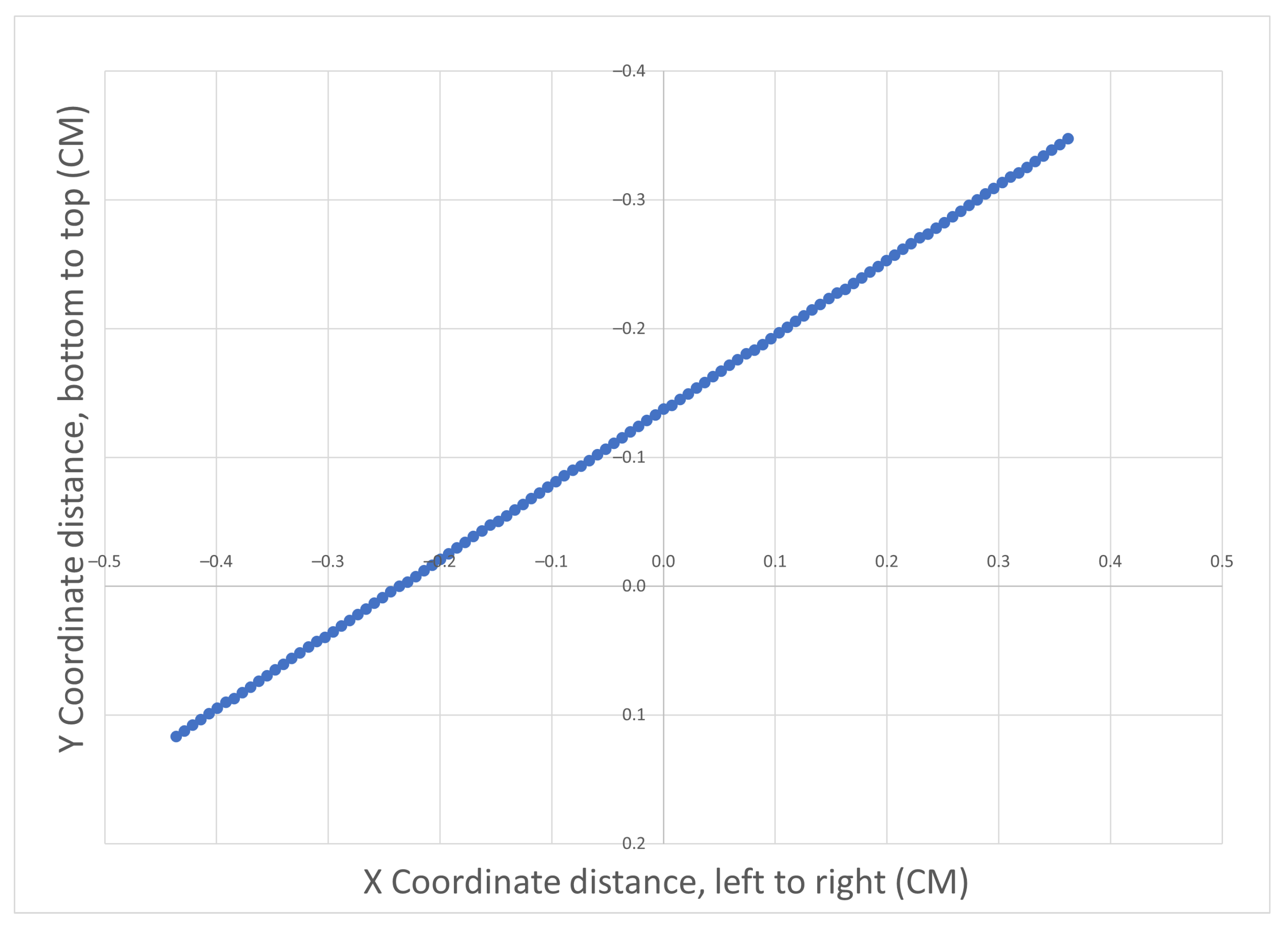
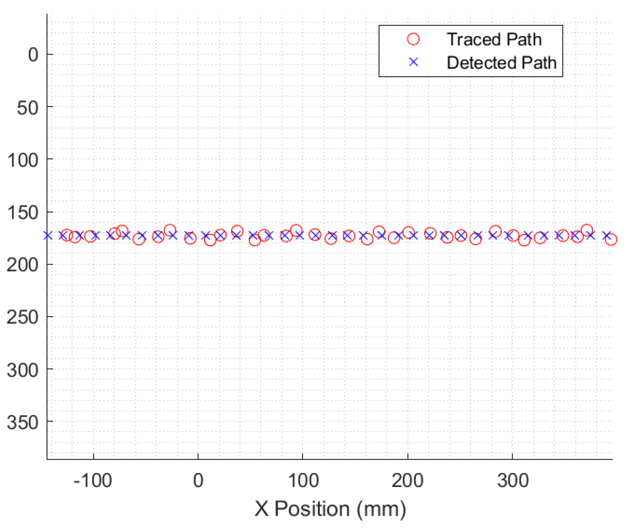
4.2.3. Feature Tracing
5. Conclusions and Future Work
Author Contributions
Funding
Data Availability Statement
Conflicts of Interest
References
- Williams, M. JOBS02: Workforce Jobs by Industry; Technical Report; Office for National Statistics: London, UK, 2019. [Google Scholar]
- Brogårdh, T. Present and future robot control development-An industrial perspective. Annu. Rev. Control. 2007, 31, 69–79. [Google Scholar] [CrossRef]
- Devlieg, R.; Szallay, T. Applied Accurate Robotic Drilling for Aircraft Fuselage. SAE Int. J. Aerosp. 2010, 3, 180–186. [Google Scholar] [CrossRef]
- Agin, G.J. Real Time Control of a Robot with a Mobile Camera; Technical Note; SRI International: Menlo Park, CA, USA, 1979. [Google Scholar]
- Hutchinson, S.; Hager, G.D.; Corke, P.I. A tutorial on visual servo control. IEEE Trans. Robot. Autom. 1996, 12, 651–670. [Google Scholar] [CrossRef] [Green Version]
- Chen, W.; Wang, X.; Liu, H.; Tang, Y.; Liu, J. Optimized combination of spray painting trajectory on 3D entities. Electronics 2019, 8. [Google Scholar] [CrossRef] [Green Version]
- Zhou, L.; Lin, T.; Chen, S.B. Autonomous acquisition of seam coordinates for arc welding robot based on visual servoing. J. Intell. Robot. Syst. Theory Appl. 2006, 47, 239–255. [Google Scholar] [CrossRef]
- Xu, D.; Wang, L.; Tan, M. Image processing and visual control method for arc welding robot. In Proceedings of the 2004 IEEE International Conference on Robotics and Biomimetics, Shenyang, China, 22–26 August 2004; pp. 727–732. [Google Scholar]
- Chen, H.; Liu, K.; Xing, G.; Dong, Y.; Sun, H.; Lin, W. A robust visual servo control system for narrow seam double head welding robot. Int. J. Adv. Manuf. Technol. 2014, 71, 1849–1860. [Google Scholar] [CrossRef]
- Zacharia, P.T.; Mariolis, I.G.; Aspragathos, N.A.; Dermatas, E.S. Visual Servoing Controller for Robot Handling Fabrics of Curved Edges. In Intelligent Production Machines and Systems—2nd I*PROMS Virtual International Conference 3–14 July 2006; Elsevier: Amsterdam, The Netherlands, 2006; pp. 301–306. [Google Scholar] [CrossRef]
- Chang, W.C.; Cheng, M.Y.; Tsai, H.J. Implementation of an Image-Based Visual Servoing structure in contour following of objects with unknown geometric models. In Proceedings of the International Conference on Control, Automation and Systems, Gwangju, Korea, 20–23 October 2013. [Google Scholar] [CrossRef]
- Gangloff, J.A.; de Mathelin, M.; Abba, G. Visual servoing of a 6 DOF manipulator for unknown 3D profile following. In Proceedings of the IEEE International Conference on Robotics and Automation, Detroit, MI, USA, 10–15 May 1999. [Google Scholar] [CrossRef]
- Boeing. Robot Painters; Boeing: Chicago, IL, USA, 2013. [Google Scholar]
- Chen, R.; Wang, G.; Zhao, J.; Xu, J.; Chen, K. Fringe Pattern Based Plane-to-Plane Visual Servoing for Robotic Spray Path Planning. IEEE/ASME Trans. Mechatronics 2018, 23, 1083–1091. [Google Scholar] [CrossRef]
- Kuka. KUKA OmniMove Moves Heavy Parts in Confined Spaces during Construction of the A380 at Airbus; Kuka: Augsburg, Germany, 2016. [Google Scholar]
- Liaqat, A.; Hutabarat, W.; Tiwari, D.; Tinkler, L.; Harra, D.; Morgan, B.; Taylor, A.; Lu, T.; Tiwari, A. Autonomous mobile robots in manufacturing: Highway Code development, simulation, and testing. Int. J. Adv. Manuf. Technol. 2019, 104, 4617–4628. [Google Scholar] [CrossRef] [Green Version]
- AMRC. AMRC’s Robot Research Cuts the Cost of Producing Aircraft Components for BAE Systems Technology to Evolve Over Time and Embrace; Technical report; AMRC: Catcliffe, UK, 2016. [Google Scholar]
- Airbus. Wing of the Future; Airbus: Leiden, The Netherlands, 2017. [Google Scholar]
- Choi, C.; Trevor, A.J.B.; Christensen, H.I. RGB-D edge detection and edge-based registration. In Proceedings of the 2013 IEEE/RSJ International Conference on Intelligent Robots and Systems, Tokyo, Japan, 3–7 November 2013; pp. 1568–1575. [Google Scholar] [CrossRef]
- Bradski, G. The OpenCV Library. Dr. Dobb’s J. Softw. Tools 2000, 120, 122–125. [Google Scholar]
- Stanford Artificial Intelligence Laboratory. Robotic Operating System; Stanford Artificial Intelligence Laboratory: Stanford, CA, USA, 2018. [Google Scholar]
- Intel. Pyrealsense2; Intel: Santa Clara, CA, USA, 2018. [Google Scholar]
- Elkady, A.; Sobh, T. Robotics Middleware: A Comprehensive Literature Survey and Attribute-Based Bibliography. J. Robot. 2012, 2012, 959013. [Google Scholar] [CrossRef] [Green Version]
- Koenig, N.; Howard, A. Design and use paradigms for Gazebo, an open-source multi-robot simulator. In Proceedings of the 2004 IEEE/RSJ International Conference on Intelligent Robots and Systems, Sendai, Japan, 28 September–2 October 2004; pp. 2149–2154. [Google Scholar] [CrossRef] [Green Version]
- Nogueira, L. Comparative Analysis Between Gazebo and V-REP Robotic Simulators. In Proceedings of the 2011 International Conference on Materials for Renewable Energy and Environment, Shanghai, China, 20–22 May 2011; pp. 1678–1683. [Google Scholar] [CrossRef]
- Canny, J. A Computational Approach to Edge Detection. IEEE Trans. Pattern Anal. Mach. Intell. 1986, 8, 679–698. [Google Scholar] [CrossRef] [PubMed]
- Rosebrock, A. Zero-Parameter, Automatic Canny Edge Detection with Python and OpenCV. 2015. Available online: https://www.pyimagesearch.com/2015/04/06/zero-parameter-automatic-canny-edge-detection-with-python-and-opencv (accessed on 11 November 2021).
- Engel, J.; Schöps, T.; Cremers, D. LSD-SLAM: Large-Scale Direct Monocular SLAM. In Computer Vision—ECCV 2014; Fleet, D., Pajdla, T., Schiele, B., Tuytelaars, T., Eds.; Springer International Publishing: Cham, Switzerland, 2014; pp. 834–849. [Google Scholar]
- Godard, C.; Aodha, O.; Firman, M.; Gabriel, J. Digging Into Self-Supervised Monocular Depth Estimation. In Proceedings of the 2019 IEEE/CVF International Conference on Computer Vision (ICCV), Seoul, Korea, 27 October–2 November 2019. [Google Scholar] [CrossRef] [Green Version]
- Patil, V.; Patil, I.; Kalaichelvi, V.; Karthikeyan, R. Extraction of Weld Seam in 3D Point Clouds for Real Time Welding Using 5 DOF Robotic Arm. In Proceedings of the 2019 5th International Conference on Control, Automation and Robotics, Beijing, China, 19–22 April 2019; pp. 727–733. [Google Scholar] [CrossRef]
- Anderson, M.; Whitcomb, P. Chapter 3: Two-Level Factorial Design. In DOE Simplified: Practical Tools for Effective Experimentation, 3rd ed.; CRC Press: Boca Raton, FL, USA, 2015; pp. 37–67. [Google Scholar]
- Manish, R.; Denis Ashok, S. Study on Effect of Lighting Variations in Edge Detection of Objects using Machine Vision System. Int. J. Eng. Res. Technol. 2016, 4, 1–5. [Google Scholar]
- Commonplace Robotics. Robotic Arm Mover6 User Guide; Commonplace Robotics GmbH: Bissendorf, Germany, 2014; pp. 1–32. [Google Scholar]
- ISO 9283:1998; Manipulating Industrial Robots—Performance Criteria and Related Test Methods. International Organization for Standardization: Geneva, Switzerland, 1998.
- da Silva Santos, K.R.; Villani, E.; de Oliveira, W.R.; Dttman, A. Comparison of visual servoing technologies for robotized aerospace structural assembly and inspection. Robot. Comput.-Integr. Manuf. 2022, 73, 102237. [Google Scholar] [CrossRef]


| Variable | Maximum (+) | Minimum (−) |
|---|---|---|
| Focus | Maximum | Minimum |
| Lighting | 862 Lux | 478 Lux |
| Aperture | 1.8 f | 16 f |
| Distance | 143 cm | 75 cm |
| Mean | |||||
|---|---|---|---|---|---|
| 0 | 4 | 8 | 18 | ||
| Var | 0.3 | 1 | 2 | 3 | 4 |
| 6 | 5 | 6 | 7 | 8 | |
| 20 | 9 | 10 | 11 | 12 | |
| 50 | 13 | 14 | 15 | 16 | |
| Experiment | Dependency Value |
|---|---|
| BC | −357 |
| AD | −224.3 |
| C | −39.4 |
| AC | −16.6 |
| ABCD | 12.3 |
| ABC | 10.9 |
| A | 10.1 |
| BD | 7.4 |
| BCD | 5.6 |
| CD | 5.2 |
| AB | −5.0 |
| D | −3.6 |
| ACD | −3.6 |
| ABD | −3.6 |
| B | −2.6 |
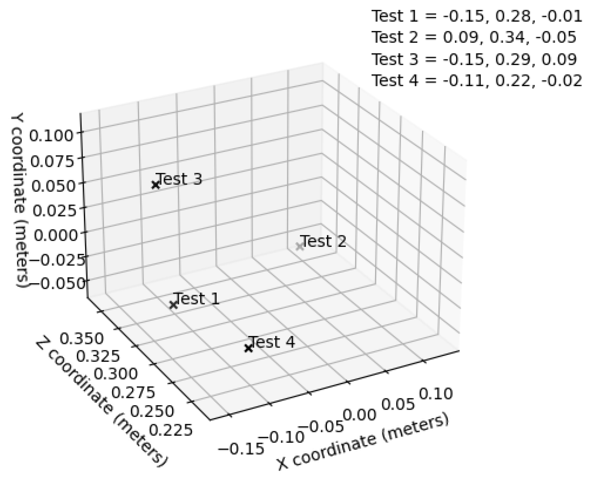
| Test Case | Feature Position in mm (X,Y,Z) | Offset in mm (X,Y,Z) |
|---|---|---|
| Test 1 | −146, −15, 276 | 50, −115, 35 |
| Test 2 | 88, −45, 34 | −3, −125, −30 |
| Test 3 | −153, 94, 289 | 1, −2, 5 |
| Test 4 | −111, −22, 216 | 0, 3, 14 |
Publisher’s Note: MDPI stays neutral with regard to jurisdictional claims in published maps and institutional affiliations. |
© 2022 by the authors. Licensee MDPI, Basel, Switzerland. This article is an open access article distributed under the terms and conditions of the Creative Commons Attribution (CC BY) license (https://creativecommons.org/licenses/by/4.0/).
Share and Cite
Clift, L.; Tiwari, D.; Scraggs, C.; Hutabarat, W.; Tinkler, L.; Aitken, J.M.; Tiwari, A. Implementation of a Flexible and Lightweight Depth-Based Visual Servoing Solution for Feature Detection and Tracing of Large, Spatially-Varying Manufacturing Workpieces. Robotics 2022, 11, 25. https://doi.org/10.3390/robotics11010025
Clift L, Tiwari D, Scraggs C, Hutabarat W, Tinkler L, Aitken JM, Tiwari A. Implementation of a Flexible and Lightweight Depth-Based Visual Servoing Solution for Feature Detection and Tracing of Large, Spatially-Varying Manufacturing Workpieces. Robotics. 2022; 11(1):25. https://doi.org/10.3390/robotics11010025
Chicago/Turabian StyleClift, Lee, Divya Tiwari, Chris Scraggs, Windo Hutabarat, Lloyd Tinkler, Jonathan M. Aitken, and Ashutosh Tiwari. 2022. "Implementation of a Flexible and Lightweight Depth-Based Visual Servoing Solution for Feature Detection and Tracing of Large, Spatially-Varying Manufacturing Workpieces" Robotics 11, no. 1: 25. https://doi.org/10.3390/robotics11010025
APA StyleClift, L., Tiwari, D., Scraggs, C., Hutabarat, W., Tinkler, L., Aitken, J. M., & Tiwari, A. (2022). Implementation of a Flexible and Lightweight Depth-Based Visual Servoing Solution for Feature Detection and Tracing of Large, Spatially-Varying Manufacturing Workpieces. Robotics, 11(1), 25. https://doi.org/10.3390/robotics11010025