Investigation of a Collisional Radiative Model for Laser-Produced Plasmas

Abstract

Plasmas of a variety of types can be described by the collisional radiative (CR) model developed by Colombant and Tonan. From the CR model, the ion distribution of a plasma at a given electron temperature and density can be found. This information is useful for further simulations, and due to this, the employment of a suitable CR model is important. Specifically, ionization bottlenecks, where there are enhanced populations of certain charge states, can be seen in these ion distributions, which in some applications are important in maintaining large amounts of a specific ion. The present work was done by implementing an accepted CR model, proposed by Colombant and Tonon, in Python and investigating the effects of variations in the ionization energy and outermost electron subshell occupancy term on the positions of ionization bottlenecks. Laser Produced Plasmas created using a Nd:YAG laser with an electron density of ∼n_e = 10²¹ cm⁻³ were the focus of this work. Plots of the collisional ionization, radiative recombination, and three-body recombination rate coefficients as well as the ion distribution and peak fractional ion population for various elements were examined. From these results, it is evident that using ionization energies from the NIST database and removing the orbital occupancy term in the CR model produced results with ionization bottlenecks in expected locations.

1. Introduction

Laser-produced plasmas (LPPs) are important to many fields of research. They have found uses in laser-induced breakdown spectroscopy [1], extreme ultraviolet lithography [2], and are laboratory scale sources of astrophysical plasmas [3,4], therefore, it is important to understand the characteristics of LPPs. In this regard, a collisional-radiative (CR) model was proposed by Colombant and Tonon to describe LPPs [5]. This CR model finds the charge state distribution for an LPP, utilizing rate equations for three dominant processes: collisional ionization, three-body recombination, and radiative recombination [5].

The CR model continues to be used to estimate charge state distributions for the emission spectra of a variety of elements, for example C (${\mathrm{Z}}_{\mathrm{A}}^{}=6$), Ge (${\mathrm{Z}}_{\mathrm{A}}^{}=32$), and Gd (${\mathrm{Z}}_{\mathrm{A}}^{}=64$) [6,7,8]. Typically in these experiments laser pulse lengths are on the order of 10 ns, with wavelengths of 1064 or 532 nm [6,7,8,9,10]. The CR model has seen further use in investigating LPPs through the three-body and radiative recombination rate coefficients [9]; and it has also been extended, for example into a time-dependent version taking into account photoionization [10]. Su et al. investigated the evolution of Al (${\mathrm{Z}}_{\mathrm{A}}^{}=13$) LPPs and, as might be expected, determined that the impact of photoionization on the charge state distribution was more important for plasmas with lower electron densities in which relative collisional ionization rates are lower [10]. The photoionization rates reported by Su et al. for Al${}^{3+}$ to Al${}^{6+}$ have orders of magnitude in the same range as the other rate coefficients. Colombant and Tonan [5] used units of cm${}^3$s${}^{-1}$ for rate coefficients for the three dominant processes and to express photoionization rates in these units Su et al. considered rates/electron number density ($n_{\mathrm{e}}$). These authors found rate coefficents for photoionization between ${10}^{-9}$ to ${10}^{-15}$ cm${}^3$s${}^{-1}$ depending on the electron temperature and density [10]. Other photoionization rates have been reported [11], but these rates describe multi-photon ionization during the formation of LPPs and thus are not applicable to the CR model considered here. However, it is noteworthy that these high photoionization rates during the laser pulse duration play a significant role in creating LPPs when the laser beam is of sufficient intensity. Comparing the order of magnitude of the photoionization rate coefficients determined by Su et al. with the multi-photon rate coefficients, clearly shows the difference between the two. For the photoionization of O (${\mathrm{Z}}_{\mathrm{A}}^{}=8$) with laser intensities on the order of ${10}^{13}$ W/cm${}^{-2}$, Sharma et al. report the multi-photon rates being between ${10}^8$ to ${10}^{10}$ s${}^{-1}$, where $n_{\mathrm{e}}$ is on the order of ${10}^{14}$ to ${10}^{15}$ cm${}^{-3}$[11], corresponding to rate coefficients between ${10}^{-6}$ to ${10}^{-5}$ cm${}^3$s${}^{-1}$. The resonant process of dielectronic recombination (DR) has recently been shown to have a significant effect upon the charge state distribution of Si (${\mathrm{Z}}_{\mathrm{A}}=14$) LPPs [12]. Due to their resonant nature, DR rates are sensitive to electron temperature. Whilst there are relatively few studies on the effect of DR on charge state distributions in plasmas at electron temperatures below 100 eV, some studies indicate that it dominates over radiative recombination [12]. It is worth bearing in mind that this recent study does not include the influence of autoionization, a resonant process that will drive the charge balance in the opposite direction to DR. The work presented here does not take into account photoionization, DR or autoionization and instead focuses on the original CR model developed by Colombant and Tonon.

The basis of the CR model is a set of analytical expressions for the rate coefficients, that have been compared to empirical formulas or experimental data [13,14]. This model was presented in 1973, and the aim of the original publication was not the CR model itself but instead an extension of it [5]. Colombant and Tonan were mainly concerned with the optimization of LPPs as heavy-ion or X-ray sources. However, the reasonable correspondence of the expressions used in the CR model with experiments has proven to be adequate, and the model is still utilized today. Despite this widespread use, little investigation into the original model has been reported. In some cases the results of the CR model are compared to other more rigorous models (such as FLYCHK [7] or a CR model based on output from HULLAC [15,16]), but this comparison is not always carried out. Thus, any inconsistencies within the CR model may go unnoticed. In the present work, the effects of altering different parameters within the CR model, namely the ionization energy of ion stage Z (${\chi }_{\mathrm{Z}}^{}$) and the number of electrons in the outermost subshell of ion stage Z (${\xi }_{\mathrm{Z}}^{}$), were examined. A representative range of elements, spanning carbon to lead, has been studied, and the main findings are presented in this article.

2. The CR Model

2.1. Limits of Applicability

The CR model described by Colombant and Tonon assumes there are three main processes in the plasma that give the ratio of two ion populations of adjacent charge states ($n_{\mathrm{Z}+1}^{}$ and $n_{\mathrm{Z}}^{}$), when the system is in a steady state [5]. The processes are collisional ionization, radiative recombination, and three-body recombination. These assumptions constrain the model to certain electron densities ($n_{\mathrm{e}}$) and temperatures ($T_{\mathrm{e}}$) [5]. The plasma must also be optically thin, and the electrons must have a Maxwellian velocity distribution [5]. The constraints on $n_{\mathrm{e}}$ and $T_{\mathrm{e}}$ come from the need for the population of the more highly charged state (Z+1) to remain steady, while the less charged state (Z) approaches its equilibrium population [5]. In other words, lower charged ion stages must reach an equilibrium population, before the populations of more highly charged ion stages significantly change. Colombant and Tonon presented a plot of this constraint, and they show for $n_{\mathrm{e}}={10}^{21}$ cm${}^{-3}$ the $T_{\mathrm{e}}$ must be at least 10 eV and for $n_{\mathrm{e}}={10}^{19}$ cm${}^{-3}$ at least 3 eV [5]. The constraint requiring an optically thin plasma necessitates $T_{\mathrm{e}}^{}\ge 30$ eV for $n_{\mathrm{e}}={10}^{21}$ cm${}^{-3}$, but the $T_{\mathrm{e}}^{}$ minimum remains the same for $n_{\mathrm{e}}={10}^{19}$ cm${}^{-3}$ [5].

Equation (1) is the electron critical density formula, with $n_{\mathrm{ec}}$ in cm${}^{-3}$ and $\lambda$ in $\mathsf{\mu }$m. From Equation (1), a wavelength of 1064 nm produces $n_{\mathrm{e}}\approx {10}^{21}$ cm${}^{-3}$, and a wavelength of 10.6 $\mathsf{\mu }$m produces $n_{\mathrm{e}}\approx {10}^{19}$ cm${}^{-3}$.

$$n_{\mathrm{ec}}=\frac{1.12\times {10}^{21}}{{\lambda }^2}\left[{\mathrm{cm}}^{-3}\right]$$

(1)

Colombant and Tonon also provide the following estimate for $T_{\mathrm{e}}$ (Equation (2)), which is valid for plasmas that are not fully ionized and have small radiation losses [5].

$$T_{\mathrm{e}}\approx 5.2\times {10}^{-6}{\mathrm{Z}}_{\mathrm{A}}^{1/5}{\left[{\lambda }^2\varphi \right]}^{3/5}\left[eV\right]$$

(2)

In Equation (2), ${\mathrm{Z}}_{\mathrm{A}}^{}$ is the target material’s atomic number, $\lambda$ is the laser wavelength in $\mathsf{\mu }$m, and $\varphi$ is the laser flux in W/cm${}^2$. Equation (2) can be used to determine indicative temperatures to find laser parameters that produce LPPs, for which the CR model is applicable. The temperature determined from the equation should fall within the temperature constrains specified by Colombant and Tonan [5] mentioned above. Since ${\mathrm{Z}}_{\mathrm{A}}^{1/5}$ is on the order of 1 to 2 for elements as heavy as Pb, $T_{\mathrm{e}}=30$ eV and $\lambda =1064$ nm in Equation (2) yields a laser flux on the order of ${10}^{11}$ W/cm${}^2$. This minimum laser flux can be achieved easily with typical Nd:YAG lasers, with laser pulse energies, pulse widths, and focal spot diameters on the order of 1 J, 10 ns, and 100 $\mathsf{\mu }$m, respectively. Where spot sizes are on the order of 10s of $\mathsf{\mu }$m the minimum laser flux is greatly exceeded [6,8,9,10]. Similarly, with $T_{\mathrm{e}}=3$ eV and $\lambda =10.6$$\mathsf{\mu }$m, a laser flux on the order of ${10}^7$ W/cm${}^2$ is found, which can be exceeded by laser energies, pulse widths, and focal spot diameters on the order of 1 J, 1 $\mathsf{\mu }$s, and a few mm, respectively. These parameters can be achieved by CO${}_2^{}$ lasers, for example as reported in [7].

The CR model no longer applies when the $n_{\mathrm{e}}^{}$ is on the order of ${10}^{17}$ cm${}^{-3}$ or smaller [5], such as in inductively coupled plasmas with $n_{\mathrm{e}}^{}$ on the order of ${10}^{14}$ cm${}^{-3}$[17], as there are not enough electron-electron collisions to ensure that the constraints of the CR model are met. This minimum order of $n_{\mathrm{e}}^{}$ magnitude (${10}^{17}$ cm${}^{-3}$) along with Equation (1) gives a limit of $\lambda \le {10}^2$$\mathsf{\mu }$m for lasers used in LPP production. Furthermore, the time to achieve a charge of Z and the time an ion is in the conduction region of the plasma must be shorter than the laser pulse [5]. Colombant and Tonon show for $n_{\mathrm{e}}^{}={10}^{21}$ cm${}^{-3}$ and $n_{\mathrm{e}}^{}={10}^{19}$ cm${}^{-3}$ the laser pulse must be greater than ${10}^{-10}-{10}^{-9}$ s and ${10}^{-8}-{10}^{-7}$ s, respectively [5]. Thus, the CR model is not applicable for LPPs from ps laser such as those in [18,19], which have $n_{\mathrm{e}}\approx {10}^{21}$ given $\lambda =1064$ nm.

2.2. Basis of the Model

The ion population ratio and rate coefficient for each process are given in Equations (3)–(6), respectively [5].

$$\frac{n_{\mathrm{Z}+1}^{}}{n_{\mathrm{Z}}^{}}=\frac{S(\mathrm{Z},T_{\mathrm{e}})}{{\alpha }_{\mathrm{r}}(\mathrm{Z}+1,T_{\mathrm{e}})+n_{\mathrm{e}}{\alpha }_{3\mathrm{b}}(\mathrm{Z}+1,T_{\mathrm{e}})}$$

(3)

$$S(\mathrm{Z},T_{\mathrm{e}})=\frac{9\times {10}^{-6}{\xi }_{\mathrm{Z}}^{}{\left(\frac{T_{\mathrm{e}}}{{\chi }_{\mathrm{Z}}^{}}\right)}^{1/2}}{{{\chi }_{\mathrm{Z}}^{}}^{3/2}(4.88+\frac{T_{\mathrm{e}}}{{\chi }_{\mathrm{Z}}^{}})}exp\left(\frac{-{\chi }_{\mathrm{Z}}^{}}{T_{\mathrm{e}}}\right)[{\mathrm{cm}}^3·{\mathrm{s}}^{-1}]$$

(4)

$${\alpha }_{\mathrm{r}}(\mathrm{Z},T_{\mathrm{e}})=5.2\times {10}^{-14}{\left(\frac{{\chi }_{\mathrm{Z}}^{}}{T_{\mathrm{e}}}\right)}^{1/2}\mathrm{Z}[0.429+\frac{1}{2}ln\left(\frac{{\chi }_{\mathrm{Z}}^{}}{T_{\mathrm{e}}}\right)+0.469{\left(\frac{T_{\mathrm{e}}}{{\chi }_{\mathrm{Z}}^{}}\right)}^{1/2}][{\mathrm{cm}}^3·{\mathrm{s}}^{-1}]$$

(5)

$${\alpha }_{3\mathrm{b}}(\mathrm{Z},T_{\mathrm{e}})=\frac{2.97\times {10}^{-27}{\xi }_{\mathrm{Z}}^{}}{T_{\mathrm{e}}{{\chi }_{\mathrm{Z}}^{}}^2(4.88+\frac{T_{\mathrm{e}}}{{\chi }_{\mathrm{Z}}^{}})}\left[{\mathrm{s}}^{-1}\right]$$

(6)

Here $n_{\mathrm{e}}$ is the electron density (in cm${}^{-3}$), ${\xi }_{\mathrm{Z}}^{}$ is the number of electrons in the outermost orbital subshell for an ion of charge Z, ${\chi }_{\mathrm{Z}}^{}$ is the ionization energy for an ion of charge Z (in $eV$), and $T_{\mathrm{e}}$ is the electron temperature (in $eV$). In the present work, $n_{\mathrm{e}}$ was set to ${10}^{21}$ cm${}^{-3}$, ${\xi }_{\mathrm{Z}}^{}$ was found using the normal rules for electron removal (removing electrons in descending order, starting with the least tightly bound electrons with the largest $nl$ values), two different sets of ${\chi }_{\mathrm{Z}}^{}$ were used (the NIST database [20] values and estimates using Equation (7), as in [5]), and $T_{\mathrm{e}}$ was either a range of values or a set value. For the ratio of the bare nucleus population over the ions with one electron remaining, a non-zero ${\chi }_{\mathrm{Z}}^{}$ for the bare nucleus is needed, since Equations (5) and (6) require this value in several places including denominators. The bare nucleus was assumed to have an ${\chi }_{\mathrm{Z}}^{}$ similar to the Bohr Hydrogen atom and was calculated as ${\chi }_{\mathrm{Z}}^{}=13.5984{\left(\mathrm{Z}\right)}^2$ [eV], with $\mathrm{Z}={\mathrm{Z}}_{\mathrm{A}}^{}$ being the charge of the bare nucleus.

The population ratio ($n_{\mathrm{Z}}^{}/n_{\mathrm{Total}}^{}$) for all charge states of an ion at a given temperature can be found, by setting the ion population for the ground state to an arbitrary value (e.g. 1), iteratively solving Equation (3) from the ground state up to the highest charge state to obtain each ion population, and then dividing each charge state’s population by the sum of all populations. Repeating this process for different temperatures and plotting the results gives an ion distribution plot of population ratio against temperature as shown in Figure 1, which shows an example charge state, or ion, distribution for Sn (${\mathrm{Z}}_{\mathrm{A}}^{}=50$). The computing requirements are not high and the work here was done using Python.

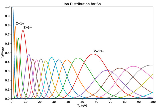
Figure 1. A Sn ion distribution generated using the traditional CR model by Colombant and Tonon [5], with different ion stages denoted by the different colored curves and the $1^{+}$, $3^{+}$, and ${13}^{+}$ ion stages marked.

2.3. Parameters Used

During the investigation some changes were made to the parameters used in the Colombant and Tonan CR model [5], which will be referred to as the traditional CR model. A major consideration was the change in determination of ${\xi }_{\mathrm{Z}}^{}$, when the phenomena known as $4f$ collapse, or contraction occurs. $4f$ contraction is where electrons in the $4f$ subshell become more tightly bound than $5p$ and $5s$ electrons, thus changing the typical electron configuration expected as the $4f$ orbital is filled before the $5p$ and $5s$ shells are completely filled [21,22]. To observe the effects of this phenomenon on the lanthanides, the electronic configurations reported in [22] were used. The outermost orbital was chosen to be the one, which appeared to lose an electron, when comparing an ion stage of charge Z to the next highest ion stage, with charge Z+1. For elements heavier than the lanthanides, the standard electron removal method was used again for simplicity.

In addition to this, the ionization energy used is an important factor within the model, but the actual values used are not reported in many of the papers using the CR model. Complicating the issue is that Colombant and Tonon provide an estimated ionization energy shown in Equation (7) [5], which will be referred to as CT ${\chi }_{\mathrm{Z}}^{}$, and small variations in the ionization energy can produce significantly different results. Within Equation (7), ${\chi }_{\mathrm{Z}}^{}$ is the ionization energy to obtain an ion of charge Z, Z is the charge of the ion, and ${\mathrm{Z}}_{\mathrm{A}}^{}$ is the atomic number of the element.

$${\chi }_{\mathrm{Z}}^{}\approx \frac{45{\mathrm{Z}}^2}{{\mathrm{Z}}_{\mathrm{A}}^{2/3}}\left[\mathrm{eV}\right]$$

(7)

2.4. Correction to the Traditional CR Model

While investigating the rate equations, a discrepancy was found in the radiative recombination rate coefficient (Equation (5)). Colombant and Tonon and their cited source for Equation (5) [23] differ from the original sources [14,24] in the power on the last $T_{\mathrm{e}}/{\chi }_{\mathrm{Z}}^{}$ term, which has a coefficient of $0.469$. Instead of a $\frac{1}{2}$ power, it is a $\frac{1}{3}$ power as shown in Equation (8) [14,24]. The $\frac{1}{3}$ power comes from the fitting of an equation to the asymptotic expansion of the Kramers-Gaunt factor for bound to free transitions [14]. Furthermore, no explanation is given for the change to $\frac{1}{2}$, nor could one be determined [23].

$${\alpha }_{\mathrm{r}}(\mathrm{Z},T_{\mathrm{e}})=5.2\times {10}^{-14}{\left(\frac{{\chi }_{\mathrm{Z}}^{}}{T_{\mathrm{e}}}\right)}^{1/2}\mathrm{Z}[0.429+\frac{1}{2}ln\left(\frac{{\chi }_{\mathrm{Z}}^{}}{T_{\mathrm{e}}}\right)+0.469{\left(\frac{T_{\mathrm{e}}}{{\chi }_{\mathrm{Z}}^{}}\right)}^{1/3}][{\mathrm{cm}}^3·{\mathrm{s}}^{-1}]$$

(8)

Changing the power to $\frac{1}{3}$ causes the ion distribution peaks to shift slightly toward higher temperatures, and Equation (8) was used for the majority of the data presented here. To differentiate this choice from the traditional CR model which uses the $\frac{1}{2}$ power, the method using the $\frac{1}{3}$ will be referred to as the standard CR model. Table 1 lists the terms used to describe the different methods and parameter configurations used. Many elements were examined and general trends are described from this examination. The elements Sn and Pb are presented as illustrative examples, as these elements show many of the important characteristic features observed in the studies of other elements.

Table 1. A list of the terms used to describe the model and parameter configurations used throughout this work, along with a brief description of each.

Name	Description
Traditional	The CR model using Equations (3)–(6)
Standard	The CR model using Equations (3), (4), (6), and (8)
NIST ${\chi }_{\mathrm{Z}}^{}$	Use of the ${\chi }_{\mathrm{Z}}^{}$ values reported by NIST [20]
CT ${\chi }_{\mathrm{Z}}^{}$	Use of ${\chi }_{\mathrm{Z}}^{}$ values calculated from Colombant and Tonon’s estimate, Equation (7) [5]
No ${\xi }_{\mathrm{Z}}^{}$	Removal of the ${\xi }_{\mathrm{Z}}^{}$ term from Equations (4) and (6)

3. Ionization Bottlenecks

A possible error and part of the impetus for this work can be seen in Figure 1. In this distribution, there are large peaks in the maximum ion population for Sn${}^{1+}$, Sn${}^{3+}$, and Sn${}^{13+}$. However, given the phenomena known as ionization bottlenecks, these peaks are not expected. An ionization bottleneck is a build up of the ion population that occurs in ion stages with a full outermost electron orbital, due to the difference between ionization energies [25]. Therefore, the peak population of an ion stage corresponding to a full outermost subshell is expected to be greater than the peak population of its neighboring ion stages, especially the one of higher charge. The electron configurations for Sn${}^{1+}$, Sn${}^{3+}$, and Sn${}^{13+}$ do not correspond to full orbitals and are instead $\left[\mathrm{Kr}\right]4d^{10}5s^{2}5p^1$, $\left[\mathrm{Kr}\right]4d^{10}5s^1$, and $\left[\mathrm{Kr}\right]4d^1$, respectively. It would be expected that ionization bottlenecks should be observed at Sn${}^{2+}$, Sn${}^{4+}$ and Sn${}^{14+}$. Examples of this discrepancy in other research can be seen in the ion distribution plots of Gd [8,26,27] and Sn [28].

4. Results and Discussion

4.1. Sn (${\mathrm{Z}}_{\mathrm{A}}^{}=50$)

Ion distributions, such as the one shown in Figure 1, were the initial basis for comparisons. To further examine the ionization bottleneck discrepancy, ion distribution curves were extended to higher temperatures (up to $5·{10}^6$ eV), and the peak fractional populations were plotted against the number of electrons in the ionization stage for different methods, as summarized in Table 1. These results are shown in Figure 2. For the peak population plots, the standard method was plotted along with the standard method without ${\xi }_{\mathrm{Z}}^{}$. In both plots of Figure 2, the standard method with the ${\xi }_{\mathrm{Z}}^{}$ term is the solid line, and the standard method without the ${\xi }_{\mathrm{Z}}^{}$ term is the dashed line. These two cases utilize the NIST ${\chi }_{\mathrm{Z}}^{}$s and the CT ${\chi }_{\mathrm{Z}}^{}$s, as shown in Figure 2a,b respectively. For each plot, the number of electrons remaining corresponding to noble gas configurations and configurations whose outermost subshell was a filled nd subshell were marked as dashed vertical lines. The vertical lines show where ionization bottlenecks are expected to occur.

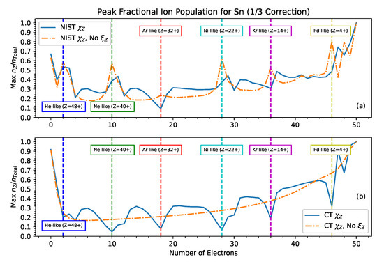
Figure 2. Plots of the peak fractional ion population for Sn calculated with the standard CR model, using Equation (3) (solid lines) and the standard CR model without the ${\xi }_{\mathrm{Z}}^{}$ term (dashed lines). Two different ${\chi }_{\mathrm{Z}}^{}$s were used, the NIST values [20] (a) and the estimated CT values from Equation (7) (b). The vertical lines mark noble gas configurations and configurations whose outermost subshell was a filled n$d^{10}$ subshell.

Using the standard CR model and NIST ${\chi }_{\mathrm{Z}}^{}$s for Sn (solid line in Figure 2a), a possible ionization bottleneck can be seen at the He-like configuration (Sn${}^{48+}$), as the peak fractional population is much larger than the more highly charged configuration (Sn${}^{49+}$) and slightly larger than the less charged configuration (Sn${}^{47+}$). All further expected ionization bottlenecks are not observed. Instead the peak fractional population for the closed subshell configurations are either much lower than their neighbors, or the lower charged neighboring configuration (Z−1) exhibits an ionization bottleneck. The Ar-like configuration (Sn${}^{32+}$) is an example of the former behaviour, with a dip, while the Ne-like, Ni-like, Kr-like, and Pd-like configurations (Sn${}^{40+}$, Sn${}^{22+}$, Sn${}^{14+}$, and Sn${}^{4+}$) are closer to the latter behaviour. Similarly, when the CT ${\chi }_{\mathrm{Z}}^{}$s are used (solid line in Figure 2b), there are dips at all of the expected ionization bottleneck locations, with only the Pd-like configuration having a significant bottleneck at a lower charged state. Removing ${\xi }_{\mathrm{Z}}^{}$ produces the expected ionization bottlenecks with the NIST ${\chi }_{\mathrm{Z}}^{}$s but removes all features with the CT ${\chi }_{\mathrm{Z}}^{}$s, as shown by the dashed lines in Figure 2a,b respectively.

While rate coefficients plots were not shown by Colombant and Tonon, they were examined here, in an effort to interpret the unusual behaviour observed for the ionization bottlenecks. The results from Equations (4), (6), and (8) were plotted for consecutive ion stages. The ground state and up to the sixth ion stage (Sn${}^{5+}$) were chosen, because several changes in the outermost occupied subshell could be observed. As with the peak fractional population plots, the NIST and CT ${\chi }_{\mathrm{Z}}^{}$s were used, with and without ${\xi }_{\mathrm{Z}}^{}$. Figure 3 shows these plots for the collisional ionization rate coefficient.

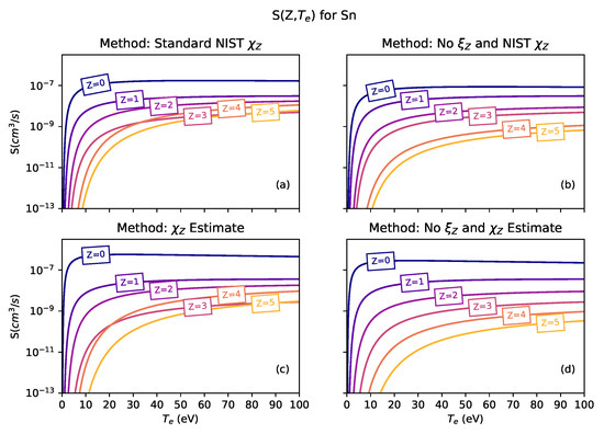
Figure 3. Plots of the collisional ionization rate coefficient for neutral Sn to Sn${}^{5+}$. Each plot was made using Equation (4) without any changes with the NIST ${\chi }_{\mathrm{Z}}^{}$s (a), without the orbital occupancy term, ${\xi }_{\mathrm{Z}}^{}$ (b), with the estimated ionization energies from Equation (7) (c), and with the estimated ionization energies and without ${\xi }_{\mathrm{Z}}^{}$ (d).

Curves for ion stages with the same outermost occupied subshell tended to group together for all of the rate coefficients. The rate equations given above indicate that the collisional ionization and three-body recombination rates decrease as ionization increases, while the radiative recombination rates would increase as ionization increased. However, as illustrated in Figure 3, some curves of ion stages with the same outermost electron orbital cross. In particular, crossing can be observed in Figure 3a,c between Sn${}^{3+}$, Sn${}^{4+}$, and Sn${}^{5+}$. An important note here is that this crossing was not seen in the radiative recombination curves; and unlike the other two rates, the radiative recombination rate does not depend on the occupancy term (${\xi }_{\mathrm{Z}}^{}$). Again, the effect of removing this occupancy was investigated. For the NIST ${\chi }_{\mathrm{Z}}^{}$s, the curve crossing observed before was no longer present in Figure 3b. For the CT ${\chi }_{\mathrm{Z}}^{}$s, removing ${\xi }_{\mathrm{Z}}^{}$ also removed the curve crossing. All rate coefficient plots followed the ionization orders seen before, but the ion stage curves were no longer clustered. Instead the first few curves corresponding to low ionization stages appeared to have larger differences than later stages, and the differences decreased in size as ionization increased. The rate coefficient differences themselves were small and gave some curves the appearance of equal spacing. This can be seen in Figure 3d for neutral Sn to Sn${}^{5+}$. This behaviour indicates that the occupancy term (${\xi }_{\mathrm{Z}}^{}$) may be associated with the appearance of ionization bottlenecks at unexpected charge states, evident in Figure 1. This association is supported by further consideration of the three-body recombination rates, as shown in Figure 4. The rates would be expected to decrease with charge state [10], however the rate for Sn${}^{3+}$ is between that for Sn${}^{6+}$ and Sn${}^{7+}$. When the occupancy (${\xi }_{\mathrm{Z}}^{}$) was removed, the exception evident in Figure 4 using the standard method was no longer present.

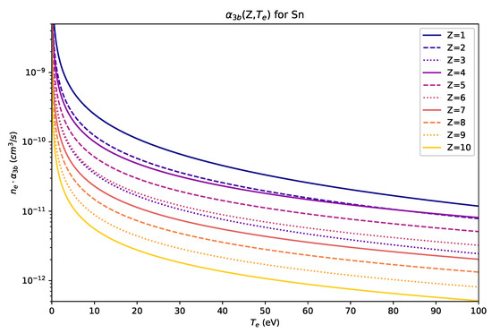
Figure 4. A plot of the 3-body recombination rate coefficient for Sn made with NIST ${\chi }_{\mathrm{Z}}^{}$s and ${\xi }_{\mathrm{Z}}^{}$ included. Here the Sn${}^{3+}$ curve is not in the same order of charge as the other curves, and is instead between the Sn${}^{6+}$ and Sn${}^{7+}$ curves. The Sn${}^{2+}$ curve can also be seen crossing the Sn${}^{4+}$ curve.

One final consideration for Sn was the population behavior of ion stages with very few to no electrons remaining, which corresponds to the far right side of the plots in Figure 2. Without the $\frac{1}{3}$ correction to Equation (5) and using the NIST ${\chi }_{\mathrm{Z}}^{}$s, with or without the occupancy factor (${\xi }_{\mathrm{Z}}^{}$), the peak population of the final stage (Z = 50${}^{+}$) was smaller than the three preceding stages (Z = 49${}^{+}$, 48${}^{+}$, and 47${}^{+}$). It would be expected that at sufficiently high temperatures bare ions would be the dominate species in the plasma. When the $\frac{1}{3}$ correction was used with the NIST ${\chi }_{\mathrm{Z}}^{}$s, the final stage had a higher peak population than the three lower charged stages, as shown in Figure 2a. In all cases using the CT ${\chi }_{\mathrm{Z}}^{}$s, the peak population of the final stage exceeded those of the neighboring states. Nevertheless, the improved behavior of the model using the NIST ${\chi }_{\mathrm{Z}}^{}$s, when $\frac{1}{3}$ (rather than $\frac{1}{2}$) was used, supports the adoption of the standard (as opposed to the traditional) model used for most of the work described here.

4.2. Common Trends Observed across the Periodic Table

The Sn plots showed many of the common trends observed in the peak fractional population and rate coefficient plots obtained for other elements investigated using the NIST ${\chi }_{\mathrm{Z}}^{}$s. In particular, the peak fractional population plots for other elements also exhibited ionization bottleneck discrepancies, peaks occurring before filled outermost subshell configurations or dips at these locations. For He-like and Ne-like configurations, these discrepancies were not seen throughout the elements examined. Instead, the expected ionization bottleneck was observed, with the peak population of these stages being greater than both of their neighbors. As atomic number increased though, the peak population of the preceding neighbor (Z−1) of the Ne-like ionization bottlenecks increased with respect to the bottleneck’s peak population. At Ru (${\mathrm{Z}}_{\mathrm{A}}^{}=44$), the peak population before the Ne-like configuration exceeded the ionization bottleneck, leading to what is observed for Sn in Figure 2a. While this trend was also seen for the He-like bottlenecks, for heavier elements the ion stages themselves went outside of the range of the plot, due to insufficient computing power and the need to maintain good resolution at lower temperatures. When the ${\xi }_{\mathrm{Z}}^{}$ term was removed, the peaks corresponding to ionization bottlenecks shifted to ion stages with full outermost orbitals.

The CT ${\chi }_{\mathrm{Z}}^{}$s also produced discrepancies throughout the elements examined. However, there were more dips at the number of electrons for a full outermost orbital than observed using the NIST ${\chi }_{\mathrm{Z}}^{}$s. This difference was often seen at lower numbers of electrons, namely He-like and Ne-like configurations. Removing ${\xi }_{\mathrm{Z}}^{}$ while using the CT ${\chi }_{\mathrm{Z}}^{}$s did not produce expected ionization bottlenecks. Instead, the peaks and dips were flattened, as shown in Figure 2b.

As with Sn, for the rate coefficient plots, generated using the NIST ${\chi }_{\mathrm{Z}}^{}$s, the curves tended to group according to their configurations’ outermost subshell. The rate coefficients also decreased or increased as ionization increased as described previously. In some cases the curves of ion stages with the same outermost electron orbital would cross, like with Sn; and no connection between the crossing point and the peak populations of the crossed curves could be found. As with Sn, in other cases one curve would not be in the ionization order for the three-body recombination plots. Again, no exceptions were observed in the radiative recombination curves. When the occupancy (${\xi }_{\mathrm{Z}}^{}$) was removed, the exceptions seen before using the standard method were no longer present, and the grouping of curves for the collisional ionization and three-body recombination curves became more distinct, as was observed for Sn.

In comparing the NIST and CT ${\chi }_{\mathrm{Z}}^{}$s, using the CT values produced the same discrepancies of crossing and out of order curves. The difference between the two methods was that the clustering of ionization stages based on the outermost electron orbital was diminished if not completely lost, when using the CT ${\chi }_{\mathrm{Z}}^{}$s. The observations for Sn, when ${\xi }_{\mathrm{Z}}^{}$ was removed, was the common trend. The curves remained in the increasing ionization order, but were not clustered; and the difference between curves appeared to be slowly decreasing.

Heavier elements continued to show the previously described trends; however, once ground state configurations have electrons in the $4f$ orbital (${\mathrm{Z}}_{\mathrm{A}}^{}\ge 58$), additional complications arise. These complications are mainly seen in configurations where the now occupied $4f$ orbital begins to be emptied and $4f$ contraction becomes relevant.

4.3. Pb (${\mathrm{Z}}_{\mathrm{A}}^{}=82$)

To illustrate the difference in behavior between the lighter elements and the lanthindes or heavier elements, Figure 5 shows peak fractional population plots for Pb, which has a ground state electronic configuration of $\left[\mathrm{Xe}\right]4f^{14}5d^{10}6s^{2}6p^2$. Continuing to use the standard electron removal method, the peak corresponding to the ionization bottleneck for an outermost electron configuration of $4f^{14}5s^{2}5p^6$ should occur at Pb${}^{14+}$ (Er-like, 68 electrons). It is clear from Figure 5a that using the standard CR model with NIST ${\chi }_{\mathrm{Z}}^{}$s produced an ionization bottleneck at a charge state Pb${}^{13+}$ rather than Pb${}^{14+}$. This discrepancy vanishes when the ${\xi }_{\mathrm{Z}}^{}$ is removed. However, the entire region between between the Pb${}^{36+}$ ion stage (Pd-like), which corresponds to a full outermost $4d$ subshell, and Pb${}^{14+}$ has no obvious ionization bottlenecks associated with the $4f$, $5s$, or $5p$ subshells. Using the occupancies (${\xi }_{\mathrm{Z}}^{}$), there is a dip at Pb${}^{22+}$ (Nd-like, 60 electrons) indicating a possible bottleneck, since this matches the discrepancies described previously for Sn and is observed for the Kr-like and Pd-like ion stages for Pb in Figure 5a. This dip could correspond to a full outermost $4f$ subshell after the $5s$ and $5p$ electrons are removed. Furthermore for the CT ${\chi }_{\mathrm{Z}}^{}$s, the dips observed at the expected bottlenecks are deeper than those observed for lighter elements. These additional observations from the Pb plots were common to period 6 elements with ${\mathrm{Z}}_{\mathrm{A}}^{}\ge 72$ (transition metals and heavier elements).

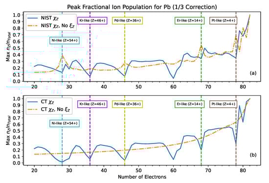
Figure 5. Plots of the peak fractional ion population Pb, calculated with the standard CR model using Equation (3) (solid lines), and from the standard CR model without the ${\xi }_{\mathrm{Z}}^{}$ term (dashed lines). Two different ${\chi }_{\mathrm{Z}}^{}$s were used, the NIST values [20] (a) and the estimated values from Equation (7) (b). The vertical lines mark noble gas configurations and configurations whose outermost subshell is a filled n$d^{10}$ subshell. The Er-like line corresponds to the electronic configuration: [Xe]$4f^{14}$.

The lanthanides exhibited the same ionization bottleneck discrepancies described for lighter elements up to Pd-like configurations (46 electrons), as discussed for Pb. At ion stages with more electrons than the Pd-like peak population trends varied, being sensitive to the ordering of shells from which electrons are stripped. This variation was most likely due to $4f$ contraction [21,22], since the value of ${\xi }_{\mathrm{Z}}^{}$ was ambiguous as the outermost subshell was no longer easily determined [22]. In other words, due to the contraction of the $4f$ orbital, ions with the same number of electrons as Xe are no longer likely to exhibit closed-shell behaviour as the ground state configuration corresponds to a mixture of open $5p$ and open 4f shells. However, if the ${\xi }_{\mathrm{Z}}^{}$ term is removed this issue becomes moot.

4.4. Gd (${\mathrm{Z}}_{\mathrm{A}}^{}=\mathit{64}$) Comparison

In order to further emphasize the importance of ${\xi }_{\mathrm{Z}}^{}$ and ${\chi }_{\mathrm{Z}}^{}$, an attempt was made to reproduce an ion distribution plot for Gadolinium (${\mathrm{Z}}_{\mathrm{A}}=64$, [Xe]$4f^{7}5d^{1}6s^2$) from another work [8]. The exact distribution could not be reproduced, but the closest agreement was achieved using the NIST ${\chi }_{\mathrm{Z}}^{}$s, with no ${\xi }_{\mathrm{Z}}^{}$ term, and without the $\frac{1}{3}$ correction to the recombination term. As described above, the removal of the occupancy term automatically negates the need to consider $4f$ contraction and the ordering of shells. The resulting plot is shown in Figure 6. In this plot ionization bottlenecks can be seen at Gd${}^{3+}$, Gd${}^{11+}$, and Gd${}^{18+}$. Gd${}^{3+}$ corresponds to the removal of the $5d^1$ and $6s^2$ electrons, whilst Gd${}^{18+}$ corresponds to a full outermost $4d$ subshell with the electronic configuration [Kr]$4d^{10}$ [22], so that these two are bottlenecks as expected. Gd${}^{11+}$ falls into the region where the ground configurations have both open $5p$ and open $4f$ shells [22], where the ground state configuration is given as [Kr]$4d^{10}5s^{2}4f^5$. This bottleneck could be attributed to the removal of all the $5p$ electrons, but it is important to keep in mind that the corresponding configurations for Gd${}^{10+}$ and Gd${}^{9+}$ are [Kr]$4d^{10}5s^{2}4f^6$ and [Kr]$4d^{10}5s^{2}5p^{2}4f^5$ respectively [22]. It is noteworthy that the Gd${}^{11+}$ bottleneck is much less distinct than those for Gd${}^{3+}$ and Gd${}^{18+}$, this being directly associated with the complex, mixed nature of the ground state configurations for ion stages in this range of charge states.

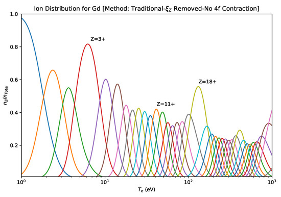
Figure 6. A Gd ion distribution generated using the traditional CR model by Colombant and Tonon using the NIST ${\chi }_{\mathrm{Z}}^{}$s, with no ${\xi }_{\mathrm{Z}}^{}$ term, and without the $\frac{1}{3}$ correction. Since the ${\xi }_{\mathrm{Z}}^{}$ was removed, whether or not 4f contraction is taken into account produces the same distribution. Here ion stages are denoted by the different colored curves, and the 3${}^{+}$, 11${}^{+}$, and 18${}^{+}$ stages are marked, due to the observed ionization bottlenecks.

4.5. Overall Findings

The effect of the ${\xi }_{\mathrm{Z}}^{}$ term within Equation (3) was investigated by comparing when the term was set to 1, effectively removing the term, and when the term was used normally. This effect was investigated using both the NIST ${\chi }_{\mathrm{Z}}^{}$s and the CT ${\chi }_{\mathrm{Z}}^{}$s. Using the NIST ${\chi }_{\mathrm{Z}}^{}$s and removing ${\xi }_{\mathrm{Z}}^{}$ produced rate coefficient plots, ion distributions, and consequently peak fractional population plots that better supported the theory of ionization bottlenecks. In other words, given the current availability of accurate ionization energy data, which were not accessible when the CR model was developed [5], it is now better to use actual ionization energies rather than to estimate them and subsequently correct for quantum effects with an occupancy factor. There is of course no physical justification for using the occupancy factor with the NIST ${\chi }_{\mathrm{Z}}^{}$s. ${\xi }_{\mathrm{Z}}^{}$ was probably introduced in an attempt to mitigate against the continuous nature of the expression used for the ionization potentials (Equation (7)) in the original CR model [5].

Examining the results using the NIST ${\chi }_{\mathrm{Z}}^{}$s, it was found that He-like and Ne-like configurations were clearly shown to be ionization bottlenecks, having peak populations greater than both the ion stage before (Z−1) and after (Z+1). However, ion stages corresponding to full outermost configurations with larger n (e.g. Ar-like, Kr-like configurations) had peak populations lower than at least one neighbor, indicating no ionization bottleneck at the anticipated configuration. Removing ${\xi }_{\mathrm{Z}}^{}$ caused these ion stages to then become ionization bottlenecks. Figure 2a. and the region below 60 electrons in Figure 5a are some examples of this. Therefore, with the NIST ${\chi }_{\mathrm{Z}}^{}$s, the ${\xi }_{\mathrm{Z}}^{}$ term seems to be the cause of the discrepancies between the charge states of observed and expected ionization bottleneck peaks.

These results suggest that the ${\xi }_{\mathrm{Z}}^{}$ term could have been an early correction factor to help account for the unrealistic smoothness of the estimated ${\chi }_{\mathrm{Z}}^{}$s. Equation (7) models processes that are quantum mechanical in nature; therefore, a term to account for an ion’s quantum state, (i.e., electronic configuration), could be needed. The introduction of such a term was discussed in the sources for Equation (4) [13,29,30]. However, the ion distributions for C and U (${\mathrm{Z}}_{\mathrm{A}}^{}=92$) presented by Colombont and Tonon [5] do not appear to have been made using the estimated ${\chi }_{\mathrm{Z}}^{}$s with the occupancy factor, since the plots were not reproduced in the present study using these parameters. The C distribution is close to one that was generated using the NIST ${\chi }_{\mathrm{Z}}^{}$s with no occupancy factor. This suggests that Colombont and Tonon [5] may have used experimentally determined ${\chi }_{\mathrm{Z}}^{}$s when they were available. This difference between the plots demonstrates the value of carefully considering what ${\chi }_{\mathrm{Z}}^{}$s are used in plasma models. In addition to this, the removal of ${\xi }_{\mathrm{Z}}^{}$, with the use of the CT estimated ${\chi }_{\mathrm{Z}}^{}$s, demonstrates the importance of utilizing the correct ${\chi }_{\mathrm{Z}}^{}$s, since under these conditions all bottleneck features are removed (as shown in Figure 2b) instead of producing the expected ionization bottlenecks.

Furthermore, within the rate coefficient plots, for some elements an ion stage curve was out of the commonly observed ion stage order. By removing ${\xi }_{\mathrm{Z}}^{}$ this order discrepancy was also removed. Some ion stage curves would also cross others. No reason could be found for this sort of crossing to occur, and when ${\xi }_{\mathrm{Z}}^{}$ was removed the curve crossing was no longer observed. Additionally, ion stages began to group according to outermost electron orbital. An example of each of these trends is shown in Figure 3a,b. Equations (4), (6), and (8) indicate that without the ${\xi }_{\mathrm{Z}}^{}$ factor, ${\chi }_{\mathrm{Z}}^{}$ is the only other variable for a given temperature ($T_{\mathrm{e}}^{}$) within the rate coefficient equations and therefore the only influence on the ion stage distributions for a fixed $n_e$. The grouping of ion stages according to the outermost electronic orbital, which are observed when the NIST ${\chi }_{\mathrm{Z}}^{}$s are used with no occupancy factor, makes sense as ${\chi }_{\mathrm{Z}}^{}$ most drastically changes between ion stages with different outermost subshells. These larger differences are in turn the reason for ionization bottlenecks [25], and therefore the observed grouping of ion stages also supports the use of experimental ${\chi }_{\mathrm{Z}}^{}$s, with no ${\xi }_{\mathrm{Z}}^{}$ term. This sole reliance of the rate equations, and thus the CR model, upon ${\chi }_{\mathrm{Z}}^{}$ underlines the benefit of using the real values of ${\chi }_{\mathrm{Z}}^{}$, which are now available [20].

5. Conclusions

In conclusion, the importance of careful consideration of the values for the ionization energies (${\chi }_{\mathrm{Z}}^{}$) and occupancy factors (${\xi }_{\mathrm{Z}}^{}$) within the traditional CR model proposed by Colombant and Tonon [5] has been shown. This point was emphasised by consideration of the charge states at which ionization bottlenecks occur. The effect of a number of different variants of the CR model were explored, revealing unphysical behaviour in rate coefficients and the associated occurrence of ionization bottlenecks at unexpected charge states. It was found that eliminating ${\xi }_{\mathrm{Z}}^{}$, removed these discrepancies, when using NIST ${\chi }_{\mathrm{Z}}^{}$ values. However, when using the CT estimated ${\chi }_{\mathrm{Z}}^{}$ values, all features indicating any ionization bottlenecks were removed if the occupancy factor was not included. A minor correction from [14,24] to the radiative recombination rate coefficient term was also found. This correction being the change of a $\frac{1}{2}$ power to a $\frac{1}{3}$ power in Equation (5).

The continuation of this work will be to compare the generated ion distributions to experimental plasmas. In this comparison, an investigation of ionization bottlenecks could also be done, since they have been the impetus for the current work with extremely visible discrepancies in the traditional CR model plots. Furthermore, the addition of the photoionization, dielectronic recombination and autoionization rate coefficients to the CR model could be tested.

References

- Kaiser, J.; Novotný, K.; Martin, M.Z.; Hrdlička, A.; Malina, R.; Hartl, M.; Adam, V.; Kizek, R. Trace elemental analysis by laser-induced breakdown spectroscopy—Biological applications. Surf. Sci. Rep. 2012, 67, 233–243. [Google Scholar] [CrossRef]
- Versolato, O.O. Physics of laser-driven tin plasma sources of EUV radiation for nanolithography. Plasma Sources Sci. Technol. 2019, 28, 83001. [Google Scholar] [CrossRef]
- Cross, J.E.; Reville, B.; Gregori, G. Scaling of magneto-quantum-radiative hydrodynamic equations: From laser-produced plasmas to astrophysics. Astrophys. J. 2014, 795, 59. [Google Scholar] [CrossRef]
- O’Sullivan, G.; Li, B.; D’Arcy, R.; Dunne, P.; Hayden, P.; Kilbane, D.; McCormack, T.; Ohashi, H.; O’Reilly, F.; Sheridan, P.; et al. Spectroscopy of highly charged ions and its relevance to EUV and soft X-ray source development. J. Phys. B At. Mol. Opt. Phys. 2015, 48, 144025. [Google Scholar] [CrossRef]
- Colombant, D.; Tonon, G.F. X-ray emission in laser-produced plasmas. J. Appl. Phys. 1973, 44, 3524–3537. [Google Scholar] [CrossRef]
- Min, Q.; Su, M.; Wang, B.; Cao, S.; Sun, D.; Dong, C. Experimental and theoretical investigation of radiation and dynamics properties in laser-produced carbon plasmas. J. Quant. Spectrosc. Radiat. Transf. 2018, 210, 189–196. [Google Scholar] [CrossRef]
- Maguire, O.; Kos, D.; O’Sullivan, G.; Sokell, E. EUV spectroscopy of optically thin Ge VI-XI plasmas in the 9–18 nm region. J. Quant. Spectrosc. Radiat. Transf. 2019, 235, 250–256. [Google Scholar] [CrossRef]
- Otsuka, T.; Kilbane, D.; White, J.; Higashiguchi, T.; Yugami, N.; Yatagai, T.; Jiang, W.; Endo, A.; Dunne, P.; O’Sullivan, G. Rare-earth plasma extreme ultraviolet sources at 6.5–6.7 nm. Appl. Phys. Lett. 2010, 97, 111503. [Google Scholar] [CrossRef]
- Wubetu, G.A.; Kelly, T.J.; Hayden, P.; Fiedorowicz, H.; Skrzeczanowski, W.; Costello, J.T. Recombination contributions to the anisotropic emission from a laser produced copper plasma. J. Phys. B At. Mol. Opt. Phys. 2020, 53, 65701. [Google Scholar] [CrossRef]
- Su, M.G.; Wang, B.; Min, Q.; Cao, S.Q.; Sun, D.X.; Dong, C.Z. Time evolution analysis of dynamics processes in laser-produced Al plasmas based on a collisional radiative model. Phys. Plasmas 2017, 24, 13302. [Google Scholar] [CrossRef]
- Sharma, A.; Slipchenko, M.N.; Shneider, M.N.; Wang, X.; Rahman, K.A.; Shashurin, A. Counting the electrons in a multiphoton ionization by elastic scattering of microwaves. Sci. Rep. 2018, 8, 1–10. [Google Scholar] [CrossRef]
- Lu, H.; Su, M.; Min, Q.; Cao, S.; He, S.; Dong, C.; Fu, Y. Effect of dielectronic recombination on charge-state distribution in laser-produced plasma based on steady-state collisional-radiative models. Plasma Sci. Technol. 2020, 22, 105001. [Google Scholar] [CrossRef]
- McWhirter, R.W.P. Spectral Intensities. In Plasma Diagnostic Techniques; Huddlestone, R.H., Leonard, S.L., Eds.; Academic Press Inc.: New York, NY, USA, 1965; pp. 201–264. [Google Scholar]
- Seaton, M.J. Radiative Recombination of Hydrogenic Ions. Mon. Not. R. Astron. Soc. 1959, 119, 81–89. [Google Scholar] [CrossRef]
- Shimada, Y.; Kawasaki, H.; Watanabe, K.; Hara, H.; Anraku, K.; Shoji, M.; Oba, T.; Matsuda, M.; Jiang, W.; Sunahara, A.; et al. Optimized highly charged ion production for strong soft X-ray sources obeying a quasi-Moseley’s law. AIP Adv. 2019, 9, 115315. [Google Scholar] [CrossRef]
- Sasaki, A.; Sunahara, A.; Nishihara, K.; Nishikawa, T. Investigation of the ionization balance of bismuth-to-tin plasmas for the extreme ultraviolet light source based on a computer-generated collisional radiative model. AIP Adv. 2016, 6, 105002. [Google Scholar] [CrossRef]
- Lee, K.; Lee, Y.; Jo, S.; Chung, C.W.; Godyak, V. Characterization of a side-type ferrite inductively coupled plasma source for large-scale processing. Plasma Sources Sci. Technol. 2008, 17, 015014. [Google Scholar] [CrossRef]
- Wu, T.; Higashiguchi, T.; Li, B.; Arai, G.; Hara, H.; Kondo, Y.; Miyazaki, T.; Dinh, T.H.; Dunne, P.; O’Reilly, F.; et al. Spectral investigation of highly ionized bismuth plasmas produced by subnanosecond Nd:YAG laser pulses. J. Phys. B At. Mol. Opt. Phys. 2016, 49, 35001. [Google Scholar] [CrossRef]
- Li, B.; Otsuka, T.; Sokell, E.; Dunne, P.; O’Sullivan, G.; Hara, H.; Arai, G.; Tamura, T.; Ono, Y.; Dinh, T.H.; et al. Characteristics of laser produced plasmas of hafnium and tantalum in the 1–7 nm region. Eur. Phys. J. D 2017, 71, 1–9. [Google Scholar] [CrossRef]
- Kramida, A.; Ralchenko, Y.; Reader, J.; NIST ASD Team. NIST Atomic Spectra Database (Ver. 5.7.1); National Institute of Standards and Technology: Gaithersburg, MD, USA, 2019. Available online: https://physics.nist.gov/asd (accessed on 12 February 2020).
- Carroll, P.K.; O’Sullivan, G. Ground-state configurations of ionic species I through XVI for Z = 57 − 74 and the interpretation of 4d − 4f emission resonances in laser-produced plasmas. Phys. Rev. A 1982, 25, 275–286. [Google Scholar] [CrossRef]
- Kilbane, D.; O’Sullivan, G. Ground-state configurations and unresolved transition arrays in extreme ultraviolet spectra of lanthanide ions. Phys. Rev. A At. Mol. Opt. Phys. 2010, 82. [Google Scholar] [CrossRef]
- Kolb, A.C.; McWhirter, R.W.P. Ionization Rates and Power Loss from θ-Pinches by Impurity Radiation. Phys. Fluids 1964, 7, 519–531. [Google Scholar] [CrossRef]
- Menzel, D.H.; Pekeris, C.L. Absorption Coefficients and Hydrogen Line Intensities. Mon. Not. R. Astron. Soc. 1935, 96, 77–110. [Google Scholar] [CrossRef]
- Attwood, D.T.; Sakdinawat, A.; Geniesse, L. X-Rays and Extreme Ultraviolet Radiation: Principles and Applications, 2nd ed.; Cambridge University Press: Cambridge, UK, 2016. [Google Scholar] [CrossRef]
- Otsuka, T.; Higashiguchi, T.; Yugami, N. Rare-Earth Plasma Beyond Extreme Ultraviolet (BEUV) Sources at 6.x nm. Electron. Commun. Jpn. 2015, 98, 52–58. [Google Scholar] [CrossRef]
- Higashiguchi, T.; Otsuka, T.; Yugami, N.; Jiang, W.; Endo, A.; Dunne, P.; Li, B.; O’Sullivan, G. Shorter-Wavelength Extreme-UV Sources below 10 nm; SPIE: Washington, DC, USA, 2011. [Google Scholar] [CrossRef]
- White, J.; Hayden, P.; Dunne, P.; Cummings, A.; Murphy, N.; Sheridan, P.; O’Sullivan, G. Simplified modeling of 13.5 nm unresolved transition array emissionof a Sn plasma and comparison with experiment. J. Appl. Phys. 2005, 98, 113301. [Google Scholar] [CrossRef]
- Drawin, H.W. Zur formelmäßigen Darstellung der Ionisierungsquerschnitte gegenüber Elektronenstoß. Zeitschrift für Physik 1961, 164, 513–521. [Google Scholar] [CrossRef]
- Thomson, J.J. XLII. Ionization by moving electrified particles. Lond. Edinb. Dublin Philos. Mag. J. Sci. 1912, 23, 449–457. [Google Scholar] [CrossRef]
© 2020 by the authors. Licensee MDPI, Basel, Switzerland. This article is an open access article distributed under the terms and conditions of the Creative Commons Attribution (CC BY) license (http://creativecommons.org/licenses/by/4.0/).