Article

Calculation of the Breit–Rosenthal Effect in Bi I

by
Tarje Arntzen Røger
and
Jonas R. Persson
*
Department of Physics, Norwegian University of Science and Technology, NO-7491 Trondheim, Norway
*
Author to whom correspondence should be addressed.
This work is based on the Master thesis of the first author.
Atoms 2024, 12(12), 72; https://doi.org/10.3390/atoms12120072
Submission received: 25 November 2024 / Revised: 12 December 2024 / Accepted: 17 December 2024 / Published: 20 December 2024

Abstract

:
Corrections to the measured nuclear magnetic moments obtained from hyperfine structure measurements include the Breit–Rosenthal effect. In this paper, we present results from calculations on Bi using the GRASP2018 code. The results indicate that the Breit–Rosenthal effect is on the order of 0.1 % fm 2 , the same order of magnitude as neighbouring elements, while some atomic states may have one order of magnitude smaller values. The ground state 6 p 3   S 3 / 2 o 4 is more sensitive to the Breit–Rosenthal effect, and hence the hyperfine anomaly, with a value of −0.25 % fm 2 .

1. Introduction

The use and study of nuclear magnetic dipole moments play a crucial role in different applications and in understanding the fundamental structure of the nucleus. Various measurement techniques for extracting nuclear magnetic dipole moments include Nuclear Magnetic Resonance (NMR), β -NMR, Atomic Beam Magnetic Resonance (ABMR) experiments, and Laser spectroscopy. These methods have specific evaluation principles and corrections, such as diamagnetism for the three former and hyperfine anomaly for the latter. While diamagnetism has been widely investigated, the hyperfine anomaly is an area of almost universal neglect. The hyperfine anomaly was originally observed when accurate measurements of the hyperfine interaction constant A and the nuclear magnetic moment became available with the advent of the ABMR method in the 1940s. The hyperfine anomaly is due to interactions that are not uniform over the nuclear volume, consisting of the Breit–Rosenthal (BR) effect [1], which describes the non-point-like nature of the nuclear charge distribution, and the Bohr–Weisskopf (BW) effect [2], which relates to the distribution over the nuclear volume of the spin and orbital angular momentum contributions to the nuclear moment. The effect of the extended charge distribution (BR) can attain values up to 25% in absolute terms, while differential variations between two neighbouring isotopes are considered to be on the order of 2 × 10 4 , which explains why it has generally been neglected. The BW effect is normally on the order of 10 2 10 3 , with exceptions up to 10% [3]. To estimate the corrections, and thus the errors, in the values of the nuclear magnetic dipole moment, we have performed calculations of the differential BR effect in Bi as a systematic continuation to calculations made in Hg [4] and Pb [5]. Even if the differential BR effect is expected to be up to an order of magnitude smaller than the BW effect, it is still important to get an estimate. It should be noted that the differential BR effect may be in the same order of magnitude as the BW effect if the different isotopes have the same spin and similar magnetic dipole moments. The BR effect was studied by Rosenberg and Stroke [6], where they calculated the differential BR effect using diffuse and Hofstadter-type charge distributions for isotope pairs ( Δ N = 2 ) in various elements. In our case, we aim to study the differential BR anomaly ( Δ B R ) over a long chain of isotopes. It is thus sensible to relate the differential BR anomaly to the change in charge radius ( δ r c 2 ) in the following form:
Δ B R = λ δ r c 2
where λ is independent of the nuclear parameters and where the change in charge radius can be obtained from tables [7] or isotope shift studies. It should be noted that this assumption is based on the first-order approximation of nuclear charge distribution. Results from Heggset and Persson in Hg [4] and Karlsen and Persson [5] in Pb indicate that this is a sensible assumption for nuclei close to the doubly magic nucleus 208Pb, where deformation is expected to be small. The objective of this study is to further expand on the previous work by Heggset and Persson on Hg [4] and Karlsen and Persson [5] on Pb to Bi, as well as to summarise the findings on the calculation of the differential BR effect.

2. Method

The computations in this study were performed using GRASP2018 [8,9], a relativistic atomic structure package, based on a combination of the multiconfigurational Dirac–Hartree–Fock (MCDHF) and relativistic configuration interaction methods [10,11]. A detailed description of the calculations can be found in the master’s thesis of the first author [12].

The States Studied in Bi
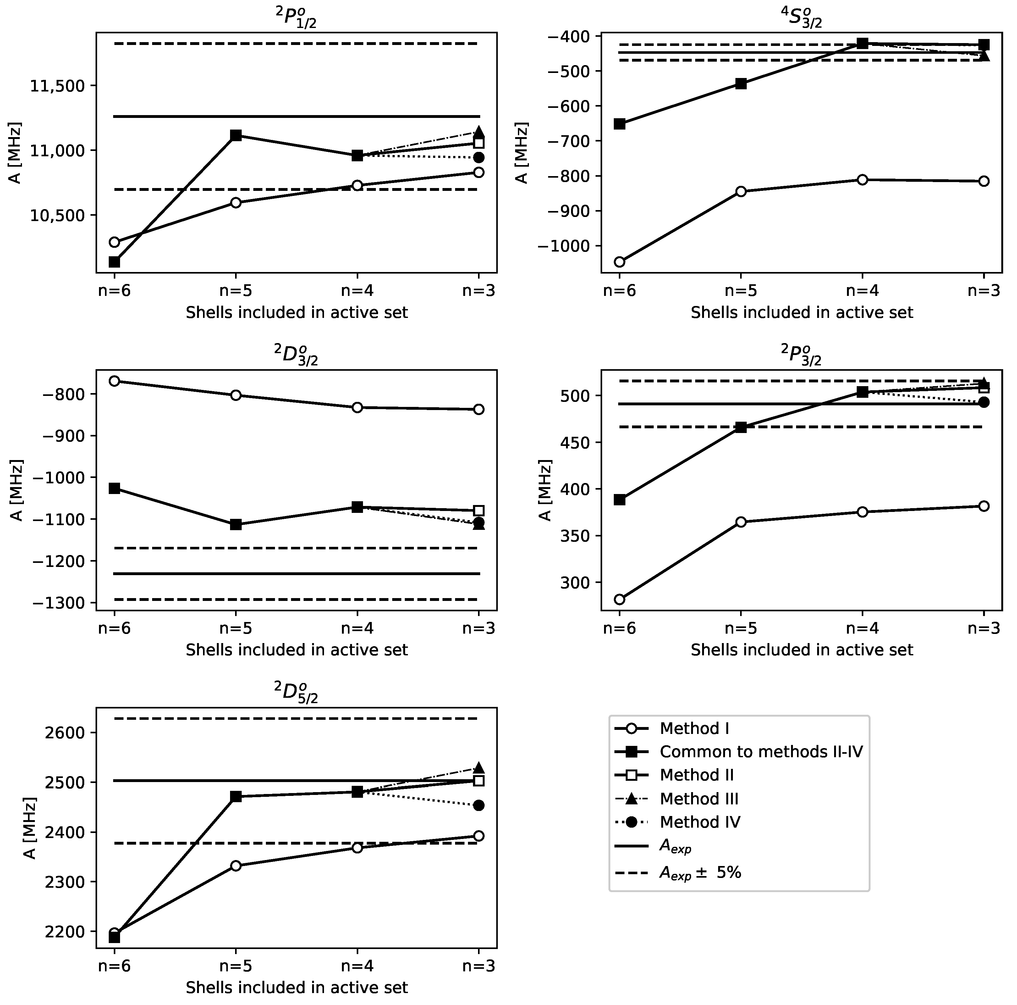
The states P 1 / 2 , 3 / 2 o 2 , D 3 / 2 , 5 / 2 o 2 , and S 3 / 2 o 4 in this study all belong to the 6 p 3 configuration. In the calculations, we used 209Bi ( I = 9 / 2 ) as the reference isotope. The calculations utilised the tabulated values for the nuclear radius, with R = 5.5211(26) fm [7] and the nuclear magnetic dipole moment μ I = 4.092(2) μ N [13]. The experimental values used (Table 1) were taken from [14].

3. Calculations

In order to obtain the values of the BR correction, a method for finding the expansion that agreed best with experimental values of the A constant was employed. As indicated by the theory, and as shown in previous studies [4,5], a good fit of A indicates a reasonable value of λ . At the same time, it is important to find the most economical method, as large-scale calculations might not be necessary. The calculations aimed to get within 5% of the experimental A constants. While previous results indicated that s p -configurations are rather insensitive to the scale of the calculations of λ [4,5], results in the p 2 -configuration in Pb [5] show a more complex picture.
The A constants for a minimal calculation (only 6 s 2 6 p 3 , multireference (MR)) gave a large deviation from the experimental A constants (see Table 2). This indicates that different expansions in the calculations are necessary. Different approaches were tested when adopting the active set approach, where orbitals are systematically evaluated. The results of the different approaches are given in Table 3 and Figure 1.
As the hyperfine interaction only involves single (S) excitations in the first order theory, a natural expansion to the multireference (MR) would be calculations on unrestricted single excitations from 6 s p 5 s p d 4 s p d f 3 s p involving four virtual layers 4 s p d f (Method I). This improved convergence, but not enough to be within 5% of the experimental values. This indicates that correlations will be of importance; thus, double (D) and even triple (T) excitations may be included. The drawbacks are the large number of Configuration state functions (CSFs) and a long calculation time.
Expanding the calculations to include some double substitutions defined Method II, where unrestricted single excitations were allowed from 6 s p 5 s p d 4 s p d f 3 s p to four virtual layers 4 s p d f g 1 h , augmented by double substitutions from 6 s p shells to the same virtual layers and double substitutions from 6 s p 5 s p d shells to one layer of virtual shells (1spdfgh). While the calculated A constants improved relative to the experimental values, the deviation is still quite large for the J = 3/2 states. To further improve this, an extra set of restricted double excitations are added: 6 s p 5 s p d 4 s p d to four virtual layers 4 s p d f g 1 h (Method III). This improvement brought the largest deviation within 10% of the experimental A constants and below 5% for the remaining four (Figure 1 and Table 4), but at the cost of computing power, as the number of CSFs increased by a factor of almost 5.
As the levels under study are all within the p 3 -configuration, one can use the approach of Bieron and Pyykkö [15] when calculating the electric field gradient to extract the nuclear quadrupole moment in 209Bi. Since the p-electrons in single excitation go to f-electrons, it might be possible to exclude active d-electrons in the core without losing too much precision while keeping the number of CSFs at an acceptable level.
This was achieved by only including the l = s , p subshells in the spectroscopic set, with unrestricted single excitations from 6 s p 5 s p 4 s p 3 s p 2 s p 1 s and unrestricted single and double excitations from 6 s p to four virtual layers 4 s p d f g 1 h and restricted single and double (SD) excitations from 6 s p 5 s p to one virtual layer 1 s p d f g h (Method IV). The latter methods (III–IV) give similar results, with good convergence (Table 2). The difference lies in the number of CSFs and, consequently, calculation time.

Calculation of BR Effect

To determine the differential BR effect, the different methods described above were used with different nuclear charge radii. For each of the methods, the change in the nuclear charge radius ( δ r c 2 ) was varied in steps of 0.25 fm2 from −1.5 to 1.0 fm2 relative to the charge radius of the reference isotope 209Bi. The BR proportionality constant λ was extracted for the five methods, and the results are given in Figure 2 and Table 4.
Method I and MR yield, as expected, different values, as these methods cannot reproduce the A constants within 5% for the J = 3/2 states. Excluding these in the discussion, we find that the values agree to a high degree. Even if the similarity of the methods can largely account for this, this indicates that the values with a high probability are close to the correct value. For the P 1 / 2 o 2 , the values vary in the range ( 0.039 , 0.040 ) , including the value for Method I, a rather small value, indicating that this state is insensitive to changes in nuclear charge radii. Since the values of Δ A are less than 5 %, a conservative error estimate should be in the same order of magnitude.
The D 5 / 2 o 2 state also shows small variations between methods for the A constants and λ , as these do not mix with other states. The values vary in the range ( 0.013 , 0.017 ) , indicating that the error should be in the same order as for the P 1 / 2 o 2 state. One also sees the insensitivity to changes in nuclear charge radii.
The J = 3/2 states show a higher degree of sensitivity towards the expansions. Method I does not reproduce the experimental A constants within 5 or 10%. Even if we were not able to get convergence to within 5% for the D 3 / 2 o 2 state for the A constant, the value of λ can still be considered to be sensible within an error of about 10%. The A constant for the S 3 / 2 o 4 and P 3 / 2 o 2 states are reproduced within or lower than 5 %. This indicates a similar error; however, the values for λ in the D 3 / 2 o 2 state vary by more than 5 %, meaning that it is sensible to increase the error.
Using these calculations, we arrive at recommended values for λ , which are given with errors in Table 5. The errors were obtained using the maximum relative errors of A constants or 5% of the calculated λ for Methods II–IV.

4. Systematics

The differential BR effect has been calculated in Hg [4], Pb [5], and now in Bi, so a comparison between these elements can be conducted. The values of λ for the different states presented in Table 6 reflect the contributions to the hyperfine structure arising from different configurations and their mixing. This indicates that the calculations of Rosenberg and Stroke [6] may be misleading, since they do not account for the mixing of states, in addition to only considering isotope pairs. In all considered cases, the absolute values of the differential BR effect is on the order of 0.1 % fm 2 , with some exceptions, notably that the 6 p 3   S 3 / 2 o 4 state in Bi is over 100% larger. This indicates consistency in the method used and possibly a general feature for elements in this region. However, the deviations should serve as a warning that a definite value of λ on the order of 0.1 % fm 2 may not be applicable for a specific state. The calculations also indicate the states that will potentially exhibit a large BW effect, as it has a similar dependency of electrons near the nucleus—that is, which transitions would be advantageous to study experimentally.

5. Conclusions

We have carried out calculations of the differential BR effect in Bi, yielding the recommended values presented in Table 5. The values are of the same order as previously published calculations [4,5]. The values are smaller than the expected values of the BW effect and confirm the practice of neglecting the BR effect, but may still be used to correct the obtained nuclear magnetic dipole moment from laser spectroscopy. Our results also suggest that the approach of Bieron and Pyykkö [15] may allow for accurate values of λ to be obtained without the need for large numbers of CSFs.

Author Contributions

Conceptualization, J.R.P.; methodology, T.A.R. and J.R.P.; software, T.A.R.; validation, J.R.P.; formal analysis, T.A.R. and J.R.P.; investigation, T.A.R. and J.R.P.; data curation, T.A.R. and J.R.P.; writing—original draft preparation, T.A.R. and J.R.P.; writing—review and editing, T.A.R. and J.R.P.; visualization, T.A.R.; supervision, J.R.P.; project administration, J.R.P. All authors have read and agreed to the published version of the manuscript.

Funding

This research received no external funding.

Data Availability Statement

The data presented in this study are available on request from the corresponding author.

Acknowledgments

The use of the HPC Cluster IDUN [16] at NTNU for the calculations is kindly acknowleged.

Conflicts of Interest

The authors declare no conflicts of interest.

References

  1. Rosenthal, J.E.; Breit, G. The Isotope Shift in Hyperfine Structure. Phys. Rev. 1932, 41, 459–470. [Google Scholar] [CrossRef]
  2. Bohr, A.; Weisskopf, V. The influence of nuclear structure on the hyperfine structure of heavy elements. Phys. Rev. 1950, 77, 94. [Google Scholar] [CrossRef]
  3. Persson, J. Table of hyperfine anomaly in atomic systems—2023. At. Data Nucl. Data Tables 2023, 154, 101589. [Google Scholar] [CrossRef]
  4. Heggset, T.; Persson, J.R. Calculation of the Differential Breit–Rosenthal Effect in the 6 s 6 p 3 P 1, 2 States of Hg. Atoms 2020, 8, 86. [Google Scholar] [CrossRef]
  5. Karlsen, M.K.; Persson, J.R. Calculation of the Differential Breit-Rosenthal Effect in Pb. Atoms 2024, 12, 5. [Google Scholar] [CrossRef]
  6. Rosenberg, H.; Stroke, H. Effect of a diffuse nuclear charge distribution on the hyperfine-structure interaction. Phys. Rev. A 1972, 5, 1992. [Google Scholar] [CrossRef]
  7. Angeli, I.; Marinova, K. Table of experimental nuclear ground state charge radii: An update. At. Data Nucl. Data Tables 2013, 99, 69–95. [Google Scholar] [CrossRef]
  8. Fischer, C.F.; Gaigalas, G.; Jönsson, P.; Bieron, J. GRASP2018—A Fortran 95 version of the general relativistic atomic structure package. Comput. Phys. Commun. 2019, 237, 184–187. [Google Scholar] [CrossRef]
  9. Jönsson, P.; Godefroid, M.; Gaigalas, G.; Ekman, J.; Grumer, J.; Li, W.; Li, J.; Brage, T.; Grant, I.P.; Bieroń, J.; et al. An Introduction to Relativistic Theory as Implemented in GRASP. Atoms 2023, 11, 7. [Google Scholar] [CrossRef]
  10. Fischer, C.F.; Godefroid, M.; Brage, T.; Jönsson, P.; Gaigalas, G. Advanced multiconfiguration methods for complex atoms: I. Energies and wave functions. J. Phys. At. Mol. Opt. Phys. 2016, 49, 182004. [Google Scholar] [CrossRef]
  11. Grant, I.P. Relativistic Quantum Theory of Atoms and Molecules: Theory and Computation; Springer Science & Business Media: Berlin/Heidelberg, Germany, 2007; Volume 40. [Google Scholar]
  12. Røger, T.A. On the Effects of a Non-Infinitesimal Nuclear Charge Distribution on the Hyperfine Spectrum of Bi I. Master’s Thesis, Norwegian University of Science and Technology (NTNU), Trondheim, Norway, 2024. [Google Scholar]
  13. Stone, N. Table of nuclear magnetic dipole and electric quadrupole moments. At. Data Nucl. Data Tables 2005, 90, 75–176. [Google Scholar] [CrossRef]
  14. Wilman, S.; Elantkowska, M.; Ruczkowski, J. Fine- and hyperfine structure semi-empirical studies of the neutral and singly ionised bismuth. Determination of the nuclear quadrupole moment of 209Bi. J. Quant. Spectrosc. Radiat. Transf. 2021, 275, 107892. [Google Scholar] [CrossRef]
  15. Bieroń, J.; Pyykkö, P. Nuclear Quadrupole Moments of Bismuth. Phys. Rev. Lett. 2001, 87, 133003. [Google Scholar] [CrossRef] [PubMed]
  16. Själander, M.; Jahre, M.; Tufte, G.; Reissmann, N. EPIC: An Energy-Efficient, High-Performance GPGPU Computing Research Infrastructure. arXiv 2019, arXiv:1912.05848. [Google Scholar]
Figure 1. Convergence for substitutions to the fourth virtual layer for methods I–IV.
Atoms 12 00072 g001
Figure 2. Linear fit of the relation δ A = λ δ r 2 for methods I, II, III, and IV, as well as for calculations using only the MR, with SD excitations.
Atoms 12 00072 g002
Table 1. Magnetic dipole hyperfine structure constants A of the 209Bi states [14].
StatesA (MHz)
S 3 / 2 o 4 −446.937 (1)
D 3 / 2 o 2 −1231.02 (15)
D 5 / 2 o 2 2502.86 (1)
P 1 / 2 o 2 11,260.2 (1.5)
P 3 / 2 o 2 491.028 (1)
Table 2. Calculated hyperfine structure constants A (in MHz) for excitations from the largest expansion to the fourth virtual layer for each method.
P 1 / 2 o 2 S 3 / 2 o 4 D 3 / 2 o 2 P 3 / 2 o 2 D 5 / 2 o 2
MR (6sp SD):10,135.23−652.01−1027.07387.692186.77
Method I:10,829.14−815.39−837.15381.592392.19
Method II:11,054.69−424.78−1079.71508.462502.79
Method III:11,142.64−456.14−1112.18512.902528.48
Method IV:10,944.31−426.49−1108.15492.922453.71
Experiment:11,260.2 (1.5)−446.937 (1)−1231.02 (15)491.028 (1)2502.86 (1)
Table 3. Summary of the different methods, with the quantity | ( A e x p A c a l c ) / A e x p | 2 = | Δ A / A e x p | 2 , summarised over all magnetic dipole interaction constants, used as an indicator for the convergence towards the experimentally measured values of the hyperfine constant along with the highest and lowest Δ A for each method.
MethodNumber of CSFs | Δ A / A e x p | 2 (%) Δ A m i n (%) Δ A m a x (%)
MR155.529.9945.88
I686591.393.8382.44
II41,72313.840.0012.29
III203,29910.921.029.65
IV29,38911.510.399.98
Table 4. Summary of all the methods for which λ were calculated. The units are [%fm−2] for λ and [%] for Δ A .
Mthd.Var. P 1 / 2 o 2 S 3 / 2 o 4 D 3 / 2 o 2 P 3 / 2 o 2 D 5 / 2 o 2
I λ −0.039−0.167−0.1310.169−0.013
Δ A 3.8382.4432.0022.294.42
II λ −0.040−0.248−0.1090.095−0.017
Δ A 1.834.9612.293.550.00
III λ −0.039−0.249−0.1100.103−0.016
Δ A 1.042.069.654.451.02
IV λ −0.039−0.253−0.1100.108−0.014
Δ A 2.814.589.980.391.96
Table 5. Recommended values of the differential Breit–Rosenthal effect in Bi.
State λ ( % fm 2 )
S 3 / 2 o 4 −0.250 (13)
D 3 / 2 o 2 −0.110 (11)
D 5 / 2 o 2 −0.016 (2)
P 1 / 2 o 2 −0.039 (2)
P 3 / 2 o 2 0.102 (6)
Table 6. Values of the differential Breit–Rosenthal effect in Hg [4], Pb [5], and Bi.
ElementState λ ( % fm 2 )
Hg 6 s 6 p     P 1 o 3 −0.11 (1)
6 s 6 p     P 2 o 3 −0.12 (1)
Pb 6 p 2     P 1 3 −0.083 (2)
6 p 2     P 2 3 −0.009 (4)
6 p 2     D 2 1 0.09 (2)
6 p 7 s     P 1 o 3 −0.065 (3)
Bi 6 p 3     S 3 / 2 o 4 −0.250 (13)
6 p 3     D 3 / 2 o 2 −0.110 (11)
6 p 3     D 5 / 2 o 2 −0.016 (2)
6 p 3     P 1 / 2 o 2 −0.039 (2)
6 p 3     P 3 / 2 o 2 0.102 (6)
Disclaimer/Publisher’s Note: The statements, opinions and data contained in all publications are solely those of the individual author(s) and contributor(s) and not of MDPI and/or the editor(s). MDPI and/or the editor(s) disclaim responsibility for any injury to people or property resulting from any ideas, methods, instructions or products referred to in the content.

