Carbon Elastic and Inelastic Stopping-Power Components for Heavy Ions at Bohr and Higher Velocities

Abstract

Carbon stopping power (SP) data for heavy ions (HIs), obtained around Bohr velocities, revealed remarkably lower values than those predicted using the SRIM/TRIM calculations/simulations. An attempt was made to extract the elastic (collisional) and inelastic (electronic) components from the available SP data obtained in experiments. A problem is that essentially, total SP is measured in experiments, whereas electronic SP values, usually presented as the results, are derived via the subtraction of the calculated collisional component from the measured values. At high HI reduced velocities $(V/v_0)/Z_{\mathrm{HI}}^{2/3}\gtrsim 0.3$ (V and $v_0$ are HI and Bohr velocities, respectively, and $Z_{\mathrm{HI}}$ is the HI atomic number), the collisional component can be neglected, whereas at Bohr velocities it becomes comparable to the electronic one. These circumstances were used to compare the experimental SP data with the SRIM/TRIM calculations/simulations and to empirically obtain corrections to the collisional and inelastic SP components.

1. Introduction

The stopping power (SP) of solids for heavy ions (HIs) passing through thin foils is an important value that may serve as a basis for the description of specific ion–atom interactions. Large amounts of SP data accrued to-date by James F. Ziegler [1] and Helmut Paul [2] allow us to compare these data with different calculations developed to reproduce the experimental data for practical usage. The statistical analysis of their applicability for HI stopping in elemental solids [2,3,4,5] shows that mean normalized deviations for SP values at the lowest range of HI energy E = 0.001–0.25 MeV/nucleon are the smallest for the SRIM code [1], as compared to other approaches.

It should, however, be noted that the considerations [2,3,4,5] dealt with the electronic component $S{P}_e$, whereas the total SP values ($S{P}_{tot}$) are measured in experiments. The latter is usually considered as the sum of electronic and nuclear $S{P}_n$ (collisional) components while analyzing the data. SRIM calculations give us both the components and show that the contribution of $S{P}_n$ to $S{P}_{tot}$ becomes significant at $E\lesssim 0.1$ MeV/nucleon. At the same time, the qualitative analysis [6] showed that the nuclear component calculated with SRIM $S{P}_n^{\mathrm{SRIM}}$ may be overestimated in its contribution to the $S{P}_{tot}$ values [7,8] for some media and HIs in the energy range of $0.01\lesssim E\lesssim 0.1$ MeV/nucleon.

According to the databases [1,2], a carbon SP data set is the largest one. In the early experiments on carbon SP measurements for HIs at Bohr [9,10,11] and higher velocities [12], the $S{P}_e$ values were determined by subtracting $S{P}_n$ from $S{P}_{tot}$, as mentioned above. The $S{P}_n$ values were calculated [9,10] or obtained with Monte Carlo (MC) simulations [11]. The measurements were carried out for HIs escaping targets within a narrow angle relative to the beam direction crossing a target (${\theta }_{\mathrm{out}}⩽1/3^{\circ }$ [9,10] and ${\theta }_{\mathrm{out}}⩽0.{17}^{\circ }$ [11]). The estimates of $S{P}_n$ contributions showed remarkable values at the lowest energies [9,10] and for relatively thick targets [11]. An intercomparison of the HI energy losses caused by the elastic collisions, as estimated with the calculations [9] and MC simulations [11,13], showed their differences from each other within a factor of 1.5–3. The $S{P}_n$ dependencies on the HI detection aperture followed from the theoretical work [13] and the analysis of the experimental data [14].

This work attempts to re-estimate the contribution of nuclear stopping to the total carbon SP for HIs at Bohr and higher velocities. A direct comparison of SP data obtained at HI velocity $V=0.8v_0$ with the results of SRIM/TRIM calculations/simulations is considered in the next section. In Section 3, total and electronic SP values as a function of the HI velocity will be compared with SRIM calculations, and nuclear SP values will be estimated. Nuclear SP estimates thus obtained will be discussed in Section 4, and some conclusions will be made in Section 5.

2. A Stopping Power Data Survey at $\mathbf{0.8}{\mathit{v}}_{\mathbf{0}}$

The available SP data at low HI velocities [9,10,11] provide a good opportunity to check their reproducibility within different approaches. The data of Lennard et al. [11] for HIs from F to U at a velocity of $0.8v_0$ were obtained using two sets of carbon targets (thicknesses $\Delta X$∼5 and ∼30 $\mathsf{\mu }$g/cm${}^2$). The velocity corresponded to the energy $E=E_{in}-\Delta E/2$ ($E_{in}$ and $\Delta E$ are the input energy and energy loss in the target of $\Delta X$ thickness, respectively). These values are listed in the respective tables [11]. In earlier data [9,10], SPs were measured for HIs from C to Y in the energy range of 0.1–1.5 MeV, which was around the $0.8v_0$ value. The measurements were performed with targets of different thickness (3.8–24.1 $\mathsf{\mu }$g/cm${}^2$). In our consideration of the data [9,10], the SP values corresponding to $0.8v_0$ were obtained via the interpolation of the tabulated $S{P}_e$, $S{P}_n$, and $\Delta X$ values.

2.1. Comparison with SRIM/TRIM Calculations/Simulations

Figure 1 shows the electronic SP values obtained in the experiments [9,10,11] and those calculated via SRIM. As one can see in the figure, SRIM calculations significantly exceed the experimental data for ions heavier than Xe. The excess corresponds to a factor of ∼2 for U ions. A possible contribution of the SRIM nuclear stopping is also shown in the figure, which is comparable with the SRIM electronic stopping for mid-heavy ions (30 $\lesssim Z_{\mathrm{HI}}\lesssim$ 62) and much smaller than the respective values for heavier ions. The reason for the inconsistencies between the experimental and calculated data could be twofold: the overestimates of the $S{P}_n$ values subtracted from $S{P}_{tot}$ obtained in the experiment [11] or/and similar overestimates in the $S{P}_e$ values calculated via SRIM.

In an attempt to test these assumptions, TRIM simulations were performed, which allowed us to extract the events corresponding to the definite range of angles for HI escaping stopping foils, and thus to simulate the conditions of the experiments [9,10,11]. In Figure 2 and Figure 3, the results of such simulations are shown for the energy distributions of Ar and Xe passed through carbon foils of the respective thicknesses. They are compared with the energy distributions obtained for these ions in the experiments [9,11]. The total energy distributions, corresponding to 10${}^5$ simulations for the ions passing through the foils, and the energy distributions for HIs escaping the foils within output angle ${\theta }_{\mathrm{out}}$, are compared with those obtained in the experiments.

As one can see in the figures, the simulations show some shifts to higher energies in the maximum positions for the distributions defined by the output angles relative to those corresponding to all angles for escaping ions. The values of these shifts are $\delta E=2.39\pm 0.31$ and $10.4\pm 3.0$ keV for the Ar and Xe distributions, respectively. With these values, $\Delta E/\Delta X$ is reduced by the same amount, 0.36 keV/($\mathsf{\mu }$g/cm${}^2$). Applying these results to possible SP measurements at all angles, one may expect an increase in the total SP values of 8.3 and 4.6% for the Ar and Xe ions, respectively. In the experiments [9,10,11], the $\Delta E$ values were determined in the same way, i.e., as the difference between the maximum positions for the input and output energy distributions. Note that in the Ar simulations, the width of the distribution determined by the output angle is larger than the one obtained in the experiment [9], although their maximum positions are close to each other. As for the Xe ions, the situation is reversed, i.e., the widths of the distributions are close to each other, although the maximum positions differ significantly. The reduced value of the output energy obtained in the Xe simulations corresponds to a larger energy loss (stopping power).

Figure 4 shows the comparisons of the $\Delta E/\Delta X$ values obtained in the experiments [9,10,11] to those obtained in TRIM simulations, and of the respective $S{P}_e$ values extracted in these experiments to those calculated via SRIM (both are shown in Figure 1). As one can see, the ${(\Delta E/\Delta X)}^{\mathrm{expt}}/{(\Delta E/\Delta X)}^{\mathrm{TRIM}}$ and $S{P}_e^{\mathrm{expt}}/S{P}_e^{\mathrm{SRIM}}$ ratios differ slightly. This circumstance means that angle cutting is insufficient to reduce the impact of nuclear stopping in the calculated/simulated values.

As was mentioned above, the data [9,10,11] were obtained with targets of varying thickness and for different output angles for the HIs escaping the targets. Differences in the experimental conditions for the data [9,10] and the data [11] could be the reason for the data inconsistencies that appeared in Figure 4. Figure 5 shows the $\Delta E/\Delta X$ values obtained with TRIM simulations and in the experiments [10,11] as a function of output angle ${\theta }_{\mathrm{out}}$ for Cu ions escaping the targets of different thicknesses. As one can see, TRIM simulations show the independence of the $\Delta E/\Delta X$ values upon ${\theta }_{\mathrm{out}}$ for thin (∼5 $\mathsf{\mu }$g/cm${}^2$) and thick (∼30 $\mathsf{\mu }$g/cm${}^2$) targets at ${\theta }_{\mathrm{out}}\gtrsim 0.{15}^{\circ }$ and $\gtrsim 0.2^{\circ }$, respectively. The experiments with thin targets show that in going from ${\theta }_{\mathrm{out}}=0.{17}^{\circ }$ to 1/3${}^{\circ }$, the $\Delta E/\Delta X$ value increases by a factor of $1.39\pm 0.12$, whereas this value does not change in the simulations. At the same time, the ratio of the $\Delta E/\Delta X$ values obtained with thick and thin targets in the TRIM simulations ($1.06\pm 0.02$) is close to the one obtained in the experiments [11] ($1.24\pm 0.11$).

Concluding this part, one can state that SRIM/TRIM calculations/simulations essentially overestimate carbon stopping powers [11] obtained for HIs at a velocity of $0.8v_0$. At the same time, the electronic SP data [9,10] for C to Y ions are in satisfactory agreement with SRIM calculations. Further, in attempts to reproduce the data [9,10,11], they are considered within the LSS [15] and in some other approaches as an alternative to SRIM. Various approximations to the nuclear SP will be also tested.

2.2. Comparison with the LSS and Other Approaches

The stopping power considered in the framework of the LSS approach [15] is treated in a similar way as within SRIM, i.e., as the sum of electronic $S{P}_e$ and nuclear $S{P}_n$ components:

$$S{P}_{tot}=S{P}_e+S{P}_n.$$

(1)

In the literature, one can find many works that are aimed at improving each of the components in order to obtain the best agreement with updated data supplied by ongoing experiments (for example, the LSS $S{P}_e$ correction is considered in [16] for polymer foils).

Figure 6 shows the same $S{P}_e$ data [9,10,11] (see Figure 1) but in comparison to the calculations according to the LSS approach, in which reduced electronic stopping power $S_e^{\mathrm{LSS}}$ is determined as

$$S_e^{\mathrm{LSS}}=K{\epsilon }^{1/2},$$

(2)

where K is given by

$$K=\frac{0.0793Z_{\mathrm{HI}}^{2/3}{Z}_t^{1/2}{(A_{\mathrm{HI}}+A_t)}^{3/2}}{A_{\mathrm{HI}}^{3/2}{A}_t^{1/2}{(Z_{\mathrm{HI}}^{2/3}+Z_t^{2/3})}^{3/4}},$$

(3)

and reduced energy $\epsilon$ is connected with HI energy E (in keV) with the expression:

$$\epsilon =\frac{32.53A_{t}E}{(A_{\mathrm{HI}}+A_t)Z_{\mathrm{HI}}{Z}_t{(Z_{\mathrm{HI}}^{2/3}+Z_t^{2/3})}^{1/2}},$$

(4)

where $Z_{\mathrm{HI}}$ and $Z_t$ are the HI and target atomic numbers, and $A_{\mathrm{HI}}$ and $A_t$ are the HI and target masses in amu.

Possible contributions of the nuclear stopping are also shown in Figure 6. They were calculated with different approximations for the reduced $S_n\left(\epsilon \right)$ function. The least $S{P}_n$ values correspond to the $S_n\left(\epsilon \right)$ approximation proposed by Ziegler [17] (designated as LSSZ in the figure):

$$\begin{array}{ccc}\hfill S_n& =& \hfill 1.7{\epsilon }^{1/2}\frac{ln[\epsilon +exp(1\left)\right]}{1+6.8\epsilon +3.4{\epsilon }^{3/2}},\phantom{1.7}0.01⩽\epsilon ⩽10;\hfill \\ \hfill S_n& =& \hfill 0.5ln\left(0.47\epsilon \right)/\epsilon ,\phantom{{\epsilon }^{1/2}0.5ln\left(0.47\epsilon \right)/\epsilon }\epsilon >10.\hfill \end{array}$$

(5)

Two other $S{P}_n$ curves correspond to $S_n\left(\epsilon \right)$ obtained with the integration of the $f\left(\eta \right)$ function using Thomas-Fermi screening (see details, for example, in [18] and below) and via the approximation to the Kr-C free electron potential [19] (designated as TF and Kr-C, respectively, in the figure). The Kr-C reduced $S_n\left(\epsilon \right)$ function has a form:

$$S_n^{\mathrm{Kr}-\mathrm{C}}=0.5ln(1+\epsilon )/(\epsilon +0.10718{\epsilon }^{0.37544}).$$

(6)

The reduced stopping power values ($S_e^{\mathrm{LSS}}$ and $S_n$) are converted to the $S{P}_e^{\mathrm{LSS}}$ and $S{P}_n$ values in MeV/(mg/cm${}^2$) with the relationship:

$$S{P}_{e/n}=S_{e/n}\frac{5.0958Z_{\mathrm{HI}}{Z}_t{A}_{\mathrm{HI}}}{A_t(A_{\mathrm{HI}}+A_t){(Z_{\mathrm{HI}}^{2/3}+Z_t^{2/3})}^{1/2}}.$$

(7)

Comparing Figure 1 and Figure 6, one can see that the $S{P}_n$ values calculated with Equations (5) and (7) give us the least contribution to the total SP values. In Figure 7, the $S{P}_e$ and $\Delta E/\Delta X$ values obtained in the experiments [9,10,11] are compared to the respective $S{P}_e^{\mathrm{LSS}}$ and $S{P}_{tot}^{\mathrm{LSS}}$ calculated values. This figure is similar to Figure 4 showing SP ratios according to SRIM calculations. As expected and seen in Figure 7, the calculations do not reproduce oscillations in $S{P}_e$ for $Z_{\mathrm{HI}}\lesssim 40$, although the LSS calculations are closer to the $S{P}_e$ data for $Z_{\mathrm{HI}}\gtrsim 40$ than the calculations obtained with SRIM. At the same time, the contributions of the nuclear stopping obtained with Equations (5) and (7) are still overestimated, as follows from the comparison in the upper panel of the figure.

In the next section, available data on the total and electronic stopping powers are considered as a function of the HI velocity, and are compared with the respective values obtained within SRIM calculations. Within this consideration, attempts are made to estimate the nuclear stopping power from such a comparison.

3. Stopping-Power Velocity Dependence

As was mentioned above, the SP data obtained in many experiments relate to the total SP values. At relatively high velocities, when nuclear stopping is negligible, these data may refer to the electronic SP component. In the low-energy SP measurements [9,10,11], it may be recalled that the experiments were conducted within the narrow range of forward angles for HIs escaping the targets. In contrast to the $S{P}_n$ component, the $S{P}_e$ component is independent of the escaping angle. Thus, the $S{P}_n$ values considered below refer to the “forward-direction” ones. In this sense, the results of the analysis [14] mentioned above showed two distinguished empirical approximations for reduced nuclear stopping, which corresponded to the “all angles” and “forward-direction” functions.

The ratios of the total SP values obtained in the experiments ($S{P}_{tot}^{\mathrm{expt}}$) and those calculated with SRIM ($S{P}_{tot}^{\mathrm{SRIM}}$) give us a general trend in the total SP dependence on the HI velocity. Figure 8 shows these ratios as a function of reduced velocity: $V_r=(V/v_0)/Z_{\mathrm{HI}}^{2/3}$ for $Z_{\mathrm{HI}}⩾20$ (V and $v_0$ are the HI and Bohr velocities, respectively). The $V_r$ parameterization was earlier used for the derivation of HI effective charges from the SP data in many works (see, for example, [12,20,21,22,23,24,25]).

As one can see in the figure, SRIM reproduces the $S{P}_{tot}^{\mathrm{expt}}$ data in general, with some deviations within the range of +20 to −15% at $V_r\gtrsim 0.2$. At $V_r\lesssim 0.15$, SRIM overestimates the $S{P}_{tot}^{\mathrm{expt}}$ values for all HIs under analysis. These inconsistencies could not be explained by the $S{P}_e^{\mathrm{SRIM}}$ overestimates (see Figure 1 and the bottom panel in Figure 4), but they are the result of the respective overestimates in the $S{P}_n^{\mathrm{SRIM}}$ values. Specific deviations of the experimental data from the calculations could be caused by specific stopping for some $Z_{\mathrm{HI}}$, which could differ from those predicted by SRIM. This circumstance requires SP data considerations for every specified ion.

3.1. Total Stopping Power Data Analysis

In Figure 9, Figure 10, Figure 11, Figure 12, Figure 13, Figure 14, Figure 15, Figure 16, Figure 17, Figure 18 and Figure 19, the ratios of total SP values obtained in experiments and those obtained in SRIM calculations are shown for HIs from Ar to U. Some details on the $S{P}_{tot}^{\mathrm{expt}}$ data used in the subsequent analysis should be mentioned. Available original data (with original errors) were preferably used in the analysis. In the absence of tabulated data in the original works, SP data were used from the database [2].

The $S{P}_{tot}^{\mathrm{expt}}/S{P}_{tot}^{\mathrm{SRIM}}$ values as a function of $V_r$ for Ar to U ions were fitted using the correction function in the framework of the weighted LSM procedure:

$$f_{tot}^{cor}\left(V_r\right)\equiv S{P}_{tot}^{\mathrm{expt}}/S{P}_{tot}^{\mathrm{SRIM}}=a_t-b_{t}exp(-k_t{V}_r),$$

(8)

where $a_t$, $b_t$, and $k_t$ are fitting parameters.

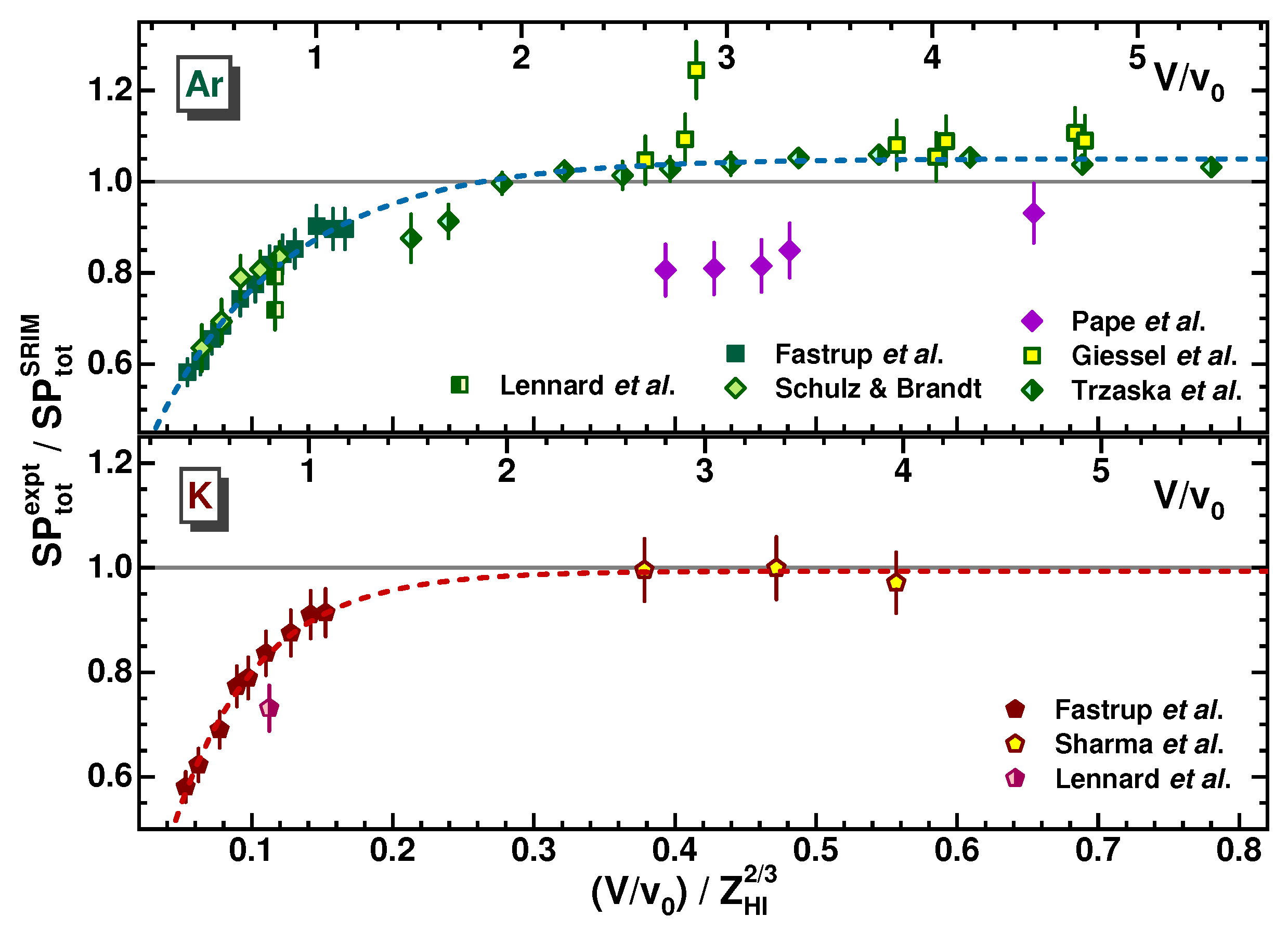
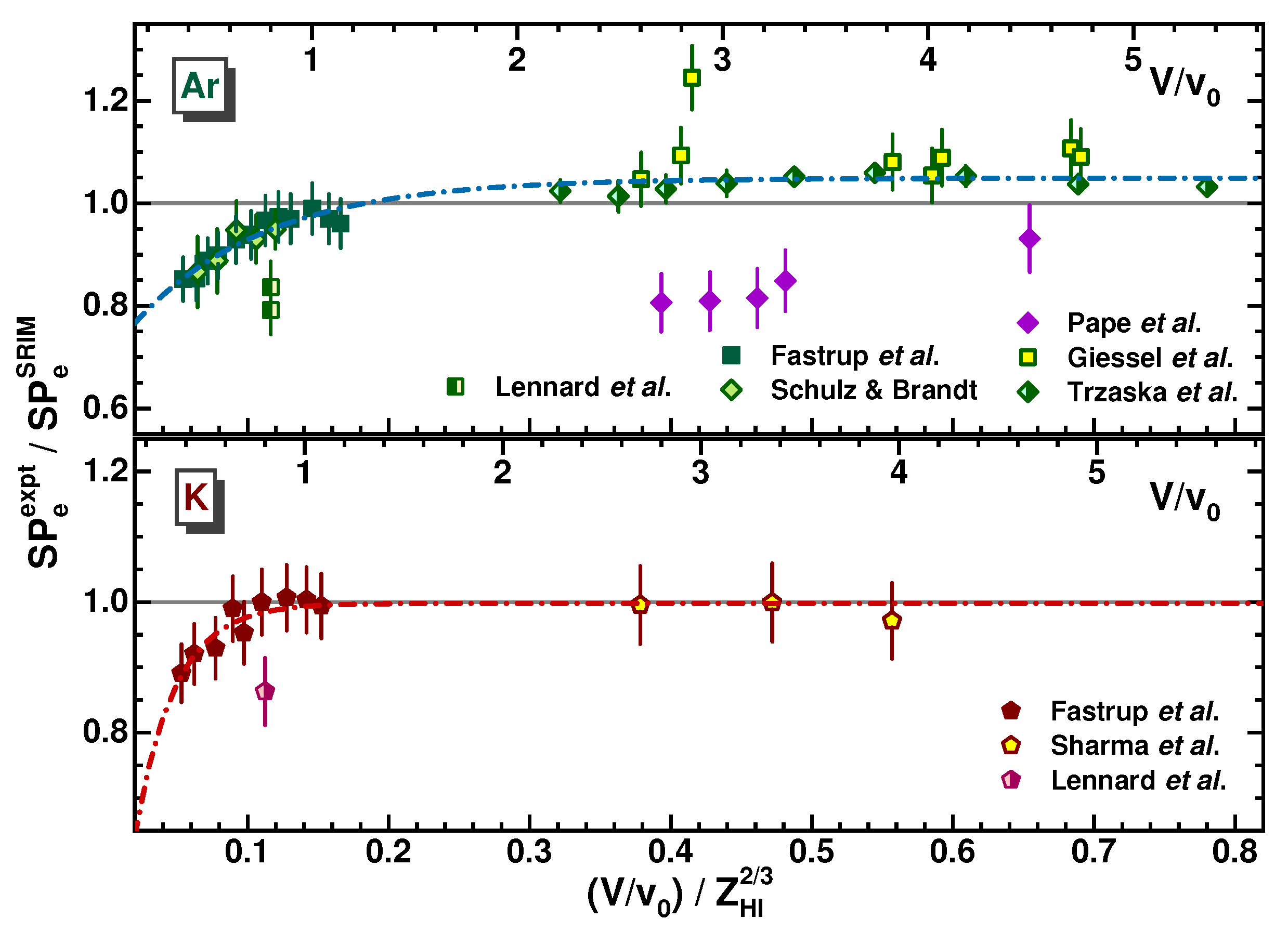
The ratios of the $S{P}_{tot}^{\mathrm{expt}}$ and $S{P}_{tot}^{\mathrm{SRIM}}$ values for Ar and K ions are shown in Figure 9. The Ar and K $S{P}_{tot}^{\mathrm{expt}}$ data were taken from the respective tables [9,11,20,26,31], whereas the Ar data obtained by Giessel et al. were taken from the database [2]. The low-velocity Ar SP data [22] were obtained using tabulated input and output energies ($E_{in}$ and $E_{out}$, respectively), target thickness $\Delta X$, and the relationship:

$$S{P}_{tot}^{\mathrm{expt}}=(E_{in}-E_{out})/\Delta X.$$

(9)

As one can see in the figure, the Ar data [26] obtained recently and the earlier data of Giessel et al. are in agreement with each other, whereas the data [20] at $V_r\gtrsim 0.4$ are inconsistent with them. The Ar and K data [11] for a thin target at $0.8v_0$ are also in disagreement with the data [9,22]. The data [11,20] were excluded from the data fit. As one could expect, adding the data [11,20] led to an increase in fitted parameter errors and in the reduced ${\chi }_r^2$ value determining fit quality. The fitting parameter values thus obtained for the Ar and K data are listed in Table 1.

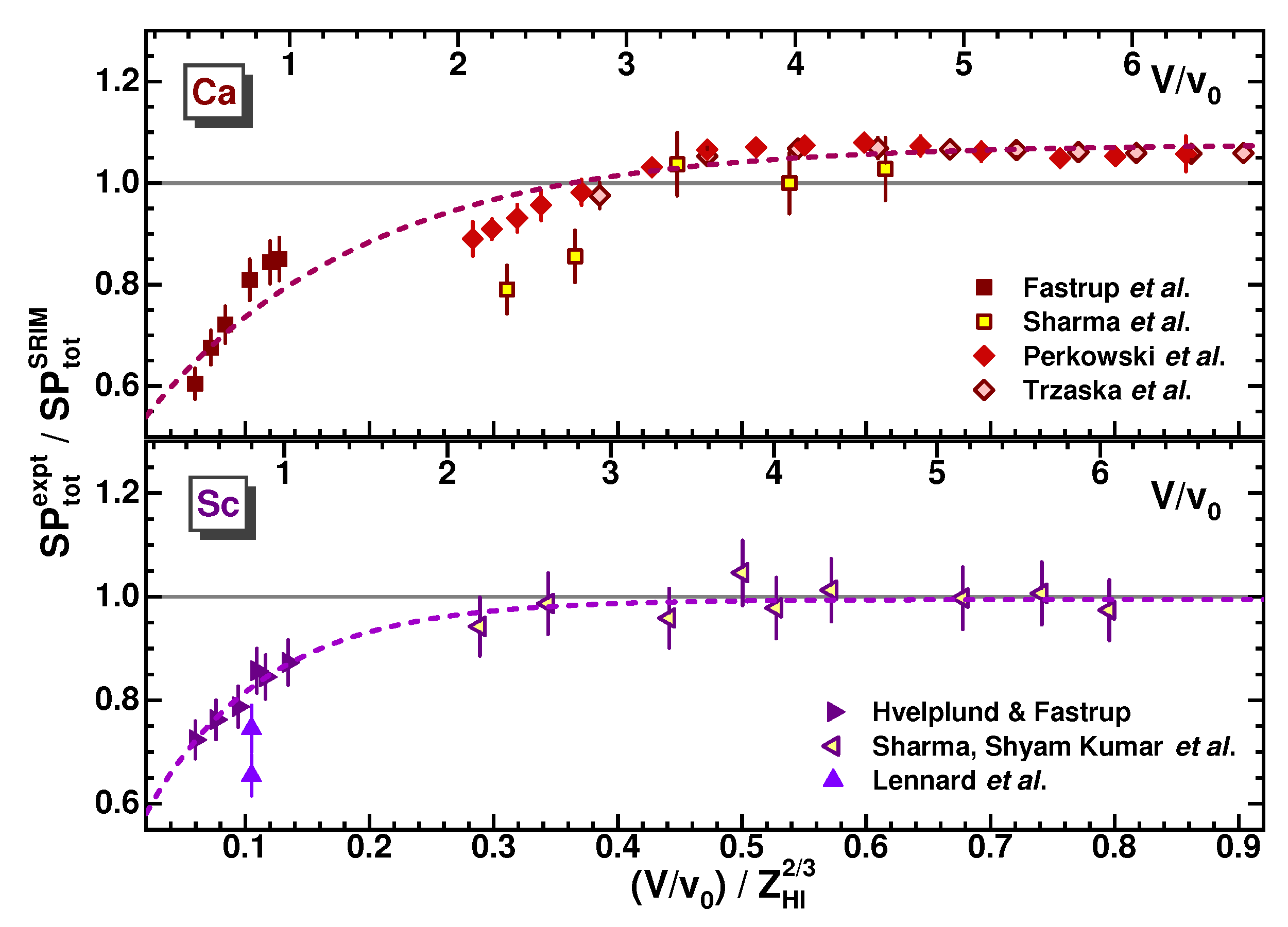
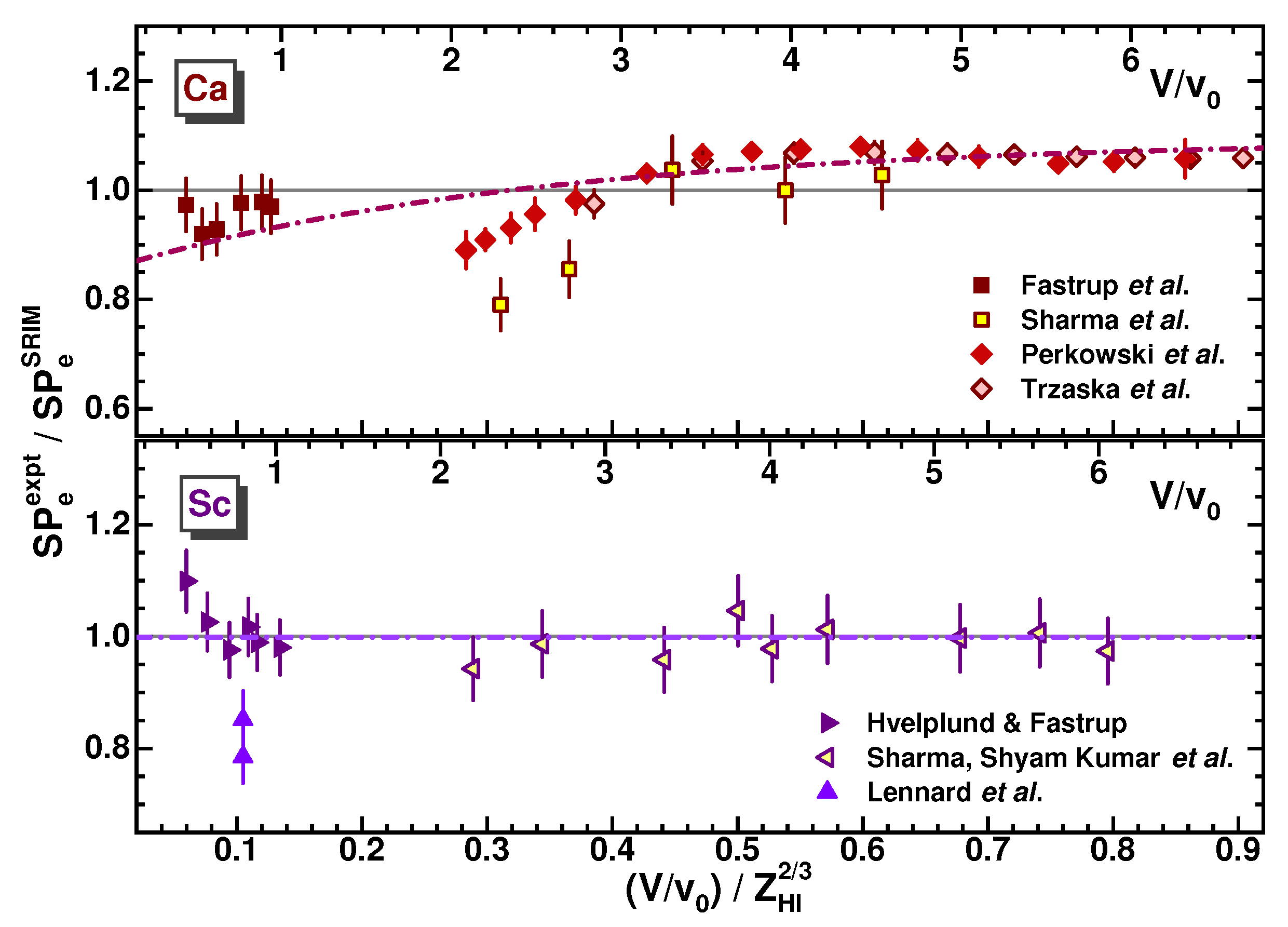
Figure 10 shows the Ca and Sc SP data [9,10,11,26,27,31,32] in comparison to SRIM calculations. As one can see, the fitting curve does not provide the match of the Ca data [9,26,27] using the function determined by Equation (8), even when omitting the data [31] at $0.3<V_r<0.4$. It is implied that the data [9] at relatively high velocities and the data [27] at relatively low velocities are reliable. In this regard, it is worth noting that the reduced ${\chi }_r^2$ value obtained for the Ca data fit (1.66) is greater than the one obtained for Sc (0.18), indicating a good match, if the data [11] were ignored. The last instances correspond to the noticeably lower SP values than those obtained in [9]. The fitting parameter values thus obtained for the Ca and Sc data are listed in Table 1.

Figure 9. The same as in Figure 8, but for the data from [2,9,10,11,20,22,26,31] for Ar and K ions only (upper and bottom panels, respectively). The results of data fits with Equation (8) are shown by dashed lines (the data [11,20] were excluded from these fits). Relative velocity $V/v_0$ is shown in the upper axes of the panels for orientation.

Figure 9. The same as in Figure 8, but for the data from [2,9,10,11,20,22,26,31] for Ar and K ions only (upper and bottom panels, respectively). The results of data fits with Equation (8) are shown by dashed lines (the data [11,20] were excluded from these fits). Relative velocity $V/v_0$ is shown in the upper axes of the panels for orientation.

Figure 10. The same as in Figure 9, but for the data from [9,10,11,26,27,31,32] for Ca and Sc ions (upper and bottom panels, respectively). See the text for details.

Figure 10. The same as in Figure 9, but for the data from [9,10,11,26,27,31,32] for Ca and Sc ions (upper and bottom panels, respectively). See the text for details.

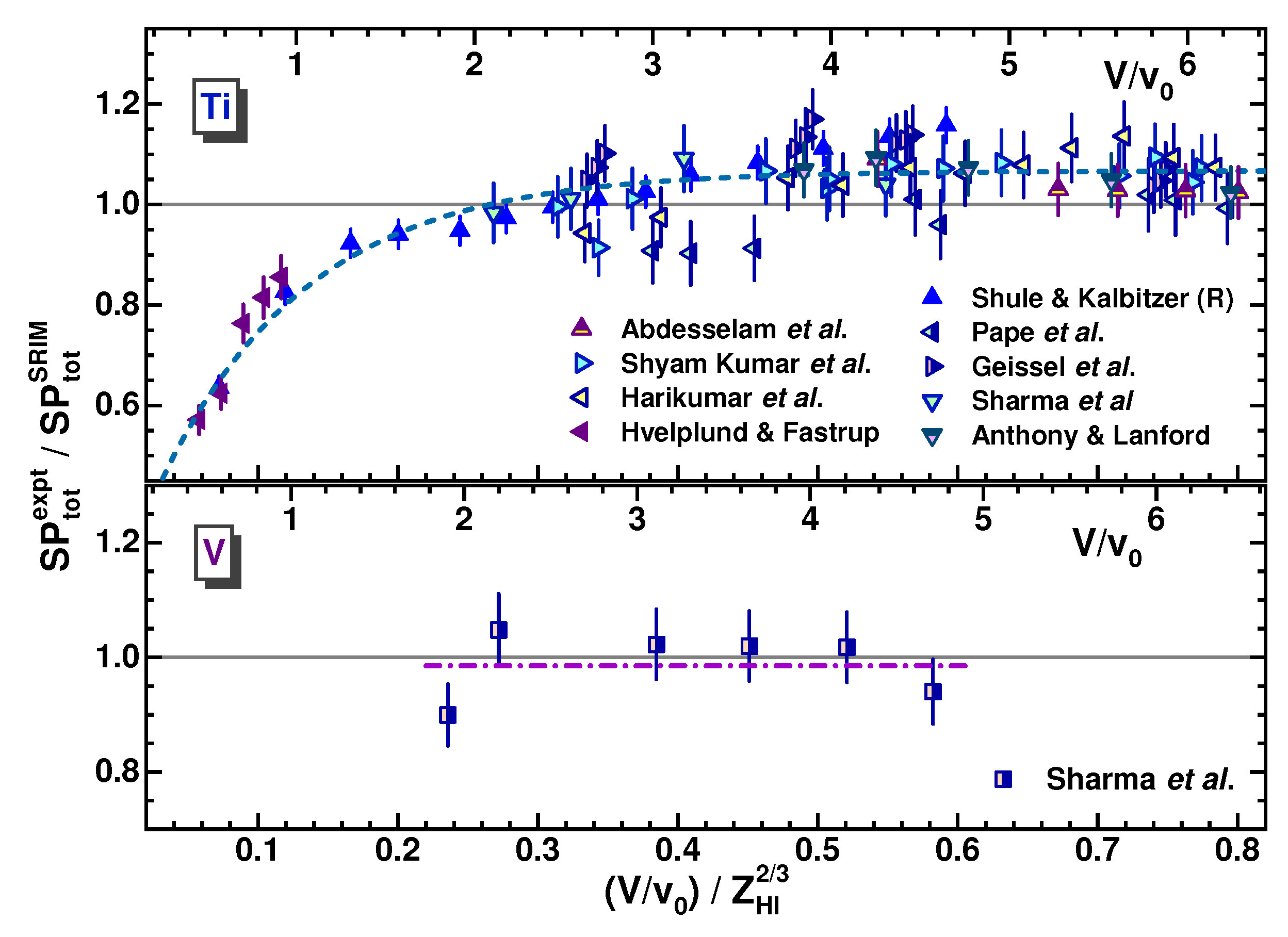
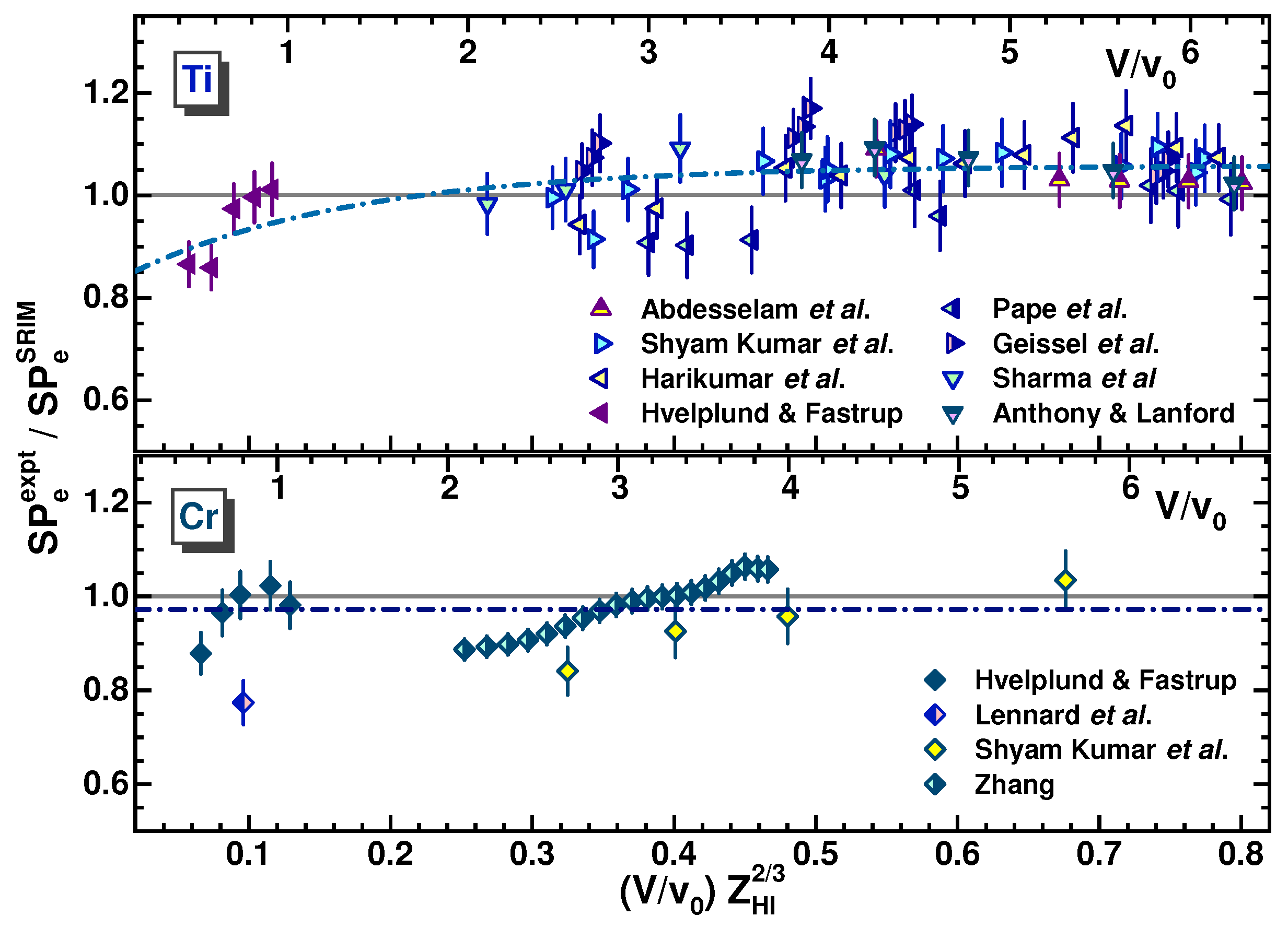
Figure 11 shows the Ti and V SP data in comparison to the SRIM calculations. The Ti data [20,21,23,31,32,33] at relatively high velocities ($V_r\gtrsim 0.3$) and those of Giessel et al. are in satisfactory agreement with each other (the data [21] and those of Giessel et al. were taken from the database [2]). The data [34] from range measurements (designated by R in the figure) agree with the low-velocity data [10] and those obtained at relatively high velocities. These data [34] were originally assigned to the electronic SP and were taken from the database [2]. They were attributed to the total SP (it seems impossible to separate the inelastic and elastic components in range measurements, considering the dominance of elastic collisions at the end of the range). The V data [31] were fitted with a constant value for the $S{P}_{tot}^{\mathrm{expt}}/S{P}_{tot}^{\mathrm{SRIM}}$ ratios. The results of data fitting for the Ti and V ions are listed in Table 1.

Figure 11. The same as in Figure 9 and Figure 10, but for the data from [2,10,20,21,23,31,32,33] for Ti and V ions (upper and bottom panels, respectively). See the text for details.

Figure 11. The same as in Figure 9 and Figure 10, but for the data from [2,10,20,21,23,31,32,33] for Ti and V ions (upper and bottom panels, respectively). See the text for details.

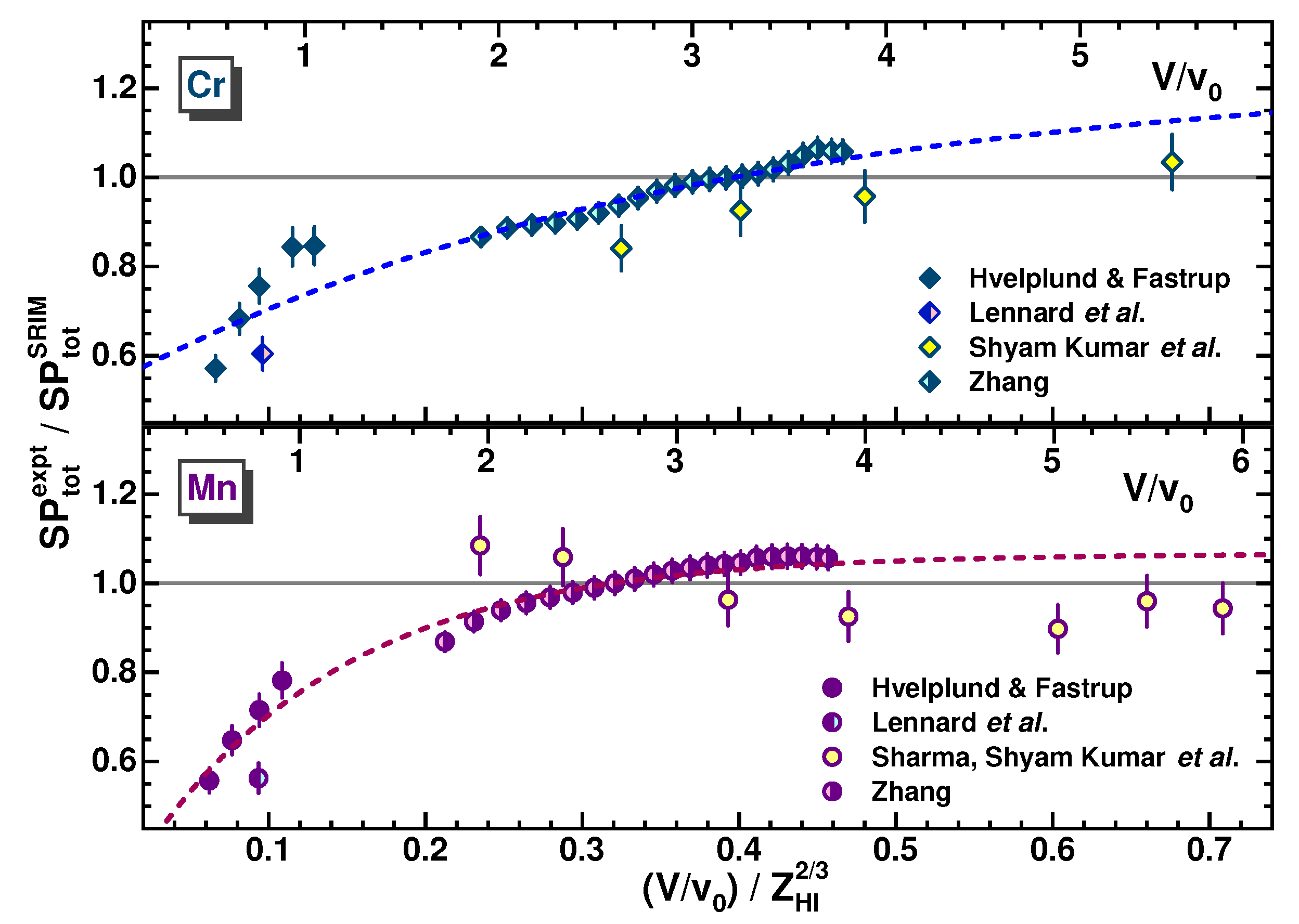
Figure 12. The same as in Figure 9, Figure 10 and Figure 11, but for the data from [2,7,10,11,31,32] for Cr and Mn ions (upper and bottom panels, respectively). See the text for details.

Figure 12. The same as in Figure 9, Figure 10 and Figure 11, but for the data from [2,7,10,11,31,32] for Cr and Mn ions (upper and bottom panels, respectively). See the text for details.

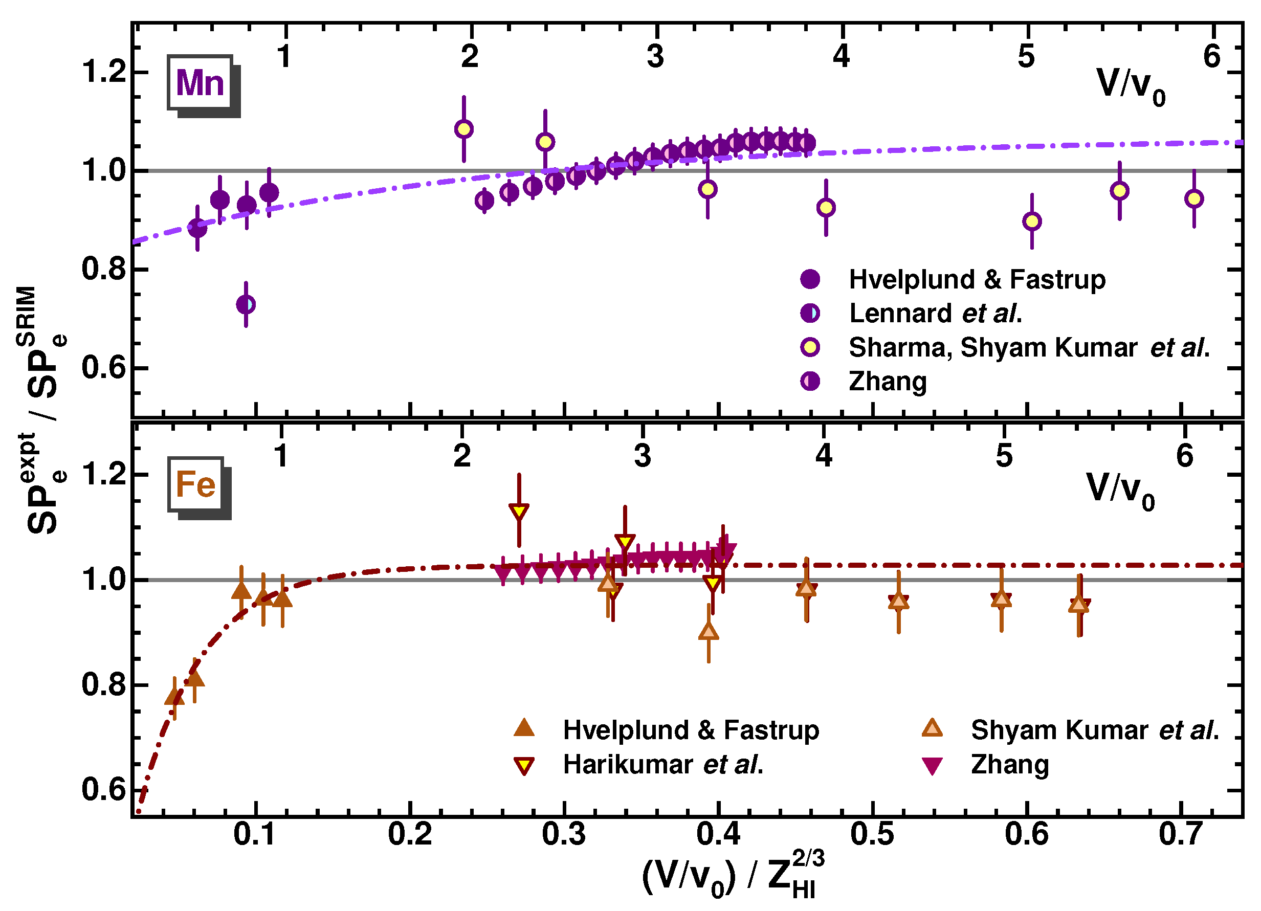
Figure 12 shows a comparison of the Cr and Mn SP data [7,10,11,31,32] to SRIM calculations (the data [7] were taken from the database [2]). The Cr data [32] at $0.3\lesssim V_r\lesssim 0.5$ and the Mn data [31] at $0.2\lesssim V_r\lesssim 0.5$ are in some disagreement with the data [7] obtained with small errors later. The fitting curve does not provide a match of the Cr data [7] with the data [10] at low velocities (similarly to the Ca data). The reason for this is that in the fitting procedure, the precision data [7] contributed more weights than the less precise ones [10,31,32]. The data [11] at $0.8v_0$ disagree with the data [10] at the same velocity, as shown in the figure, and were ignored in the fitting procedure. The results of the fitting are listed in Table 1.

Table 1. Fitting parameter values $a_t$, $b_t$, and $k_t$ as obtained for Ar to U ratios $S{P}_{tot}^{\mathrm{expt}}/S{P}_{tot}^{\mathrm{SRIM}}$ fitted with Equation (8). The ion symbols and ranges of Equation (8) applicability for specified ions are listed in the first and last columns, respectively. The results of data fitting are shown in Figure 9, Figure 10, Figure 11, Figure 12, Figure 13, Figure 14, Figure 15, Figure 16, Figure 17, Figure 18 and Figure 19.

Ion	${\mathit{a}}_{\mathit{t}}$	${\mathit{b}}_{\mathit{t}}$	${\mathit{k}}_{\mathit{t}}$	${\mathit{V}}_{\mathit{r}}$ Range
Ar 1	$1.0502\pm 0.0063$	$0.829\pm 0.061$	$10.62\pm 0.94$	0.05–0.8
K 2	$0.9934\pm 0.0105$	$1.027\pm 0.055$	$16.71\pm 1.05$	0.05–0.6
Ca 3	$1.0764\pm 0.0087$	$0.601\pm 0.045$	$5.69\pm 0.67$	0.06–0.9
Sc 2	$0.9946\pm 0.0095$	$0.511\pm 0.062$	$10.49\pm 1.60$	0.06–0.8
Ti	$1.0672\pm 0.0085$	$0.827\pm 0.061$	$9.46\pm 0.96$	0.06–0.8
V	$0.9852\pm 0.0274$			0.2–0.6
Cr 2	$1.2383\pm 0.1157$	$0.700\pm 0.089$	$2.72\pm 0.92$	0.06–0.7
Mn 2	$1.0664\pm 0.0193$	$0.786\pm 0.064$	$7.75\pm 1.14$	0.06–0.7
Fe	$1.0311\pm 0.0065$	$1.380\pm 0.149$	$18.02\pm 1.96$	0.04–0.7
Co	$1.0167\pm 0.0075$	$1.140\pm 0.050$	$12.69\pm 0.88$	0.04–0.5
Cu 2	$1.0605\pm 0.0058$	$1.874\pm 0.144$	$18.75\pm 1.32$	0.05–0.8
Ge	$1.0122\pm 0.0117$	$1.827\pm 0.142$	$19.81\pm 1.56$	0.04–0.9
Br	$1.1261\pm 0.0081$	$1.352\pm 0.070$	$13.67\pm 0.86$	0.04–0.9
Kr 4	$1.0856\pm 0.0075$	$1.326\pm 0.115$	$14.51\pm 1.49$	0.04–0.8
Y	$1.1794\pm 0.0141$	$1.127\pm 0.133$	$10.92\pm 2.08$	0.04–0.8
Ag	$1.0129\pm 0.0130$	$0.847\pm 0.332$	$11.70\pm 6.67$	0.06–0.7
I	$1.0786\pm 0.0069$			0.2–0.6
Xe	$1.0668\pm 0.0090$	$1.140\pm 0.083$	$12.46\pm 1.19$	0.05–0.8
Au	$0.9718\pm 0.0174$	$7.44\pm 7.48$	$56.8\pm 23.4$	0.04–0.4
Pb	$1.1008\pm 0.0263$	$1.335\pm 0.105$	$13.38\pm 2.40$	0.04–0.8
U	$1.0687\pm 0.0067$	$1.711\pm 0.102$	$21.28\pm 1.42$	0.04–0.8

¹ Without the data [11,20] (see the text). ² Without the data [11] (see the text). ³ Without the data [31] at $0.3<V_r<0.4$ (see the text). ⁴ Without the data [20] (see the text).

Table 1. Fitting parameter values $a_t$, $b_t$, and $k_t$ as obtained for Ar to U ratios $S{P}_{tot}^{\mathrm{expt}}/S{P}_{tot}^{\mathrm{SRIM}}$ fitted with Equation (8). The ion symbols and ranges of Equation (8) applicability for specified ions are listed in the first and last columns, respectively. The results of data fitting are shown in Figure 9, Figure 10, Figure 11, Figure 12, Figure 13, Figure 14, Figure 15, Figure 16, Figure 17, Figure 18 and Figure 19.

Ion	${\mathit{a}}_{\mathit{t}}$	${\mathit{b}}_{\mathit{t}}$	${\mathit{k}}_{\mathit{t}}$	${\mathit{V}}_{\mathit{r}}$ Range
Ar 1	$1.0502\pm 0.0063$	$0.829\pm 0.061$	$10.62\pm 0.94$	0.05–0.8
K 2	$0.9934\pm 0.0105$	$1.027\pm 0.055$	$16.71\pm 1.05$	0.05–0.6
Ca 3	$1.0764\pm 0.0087$	$0.601\pm 0.045$	$5.69\pm 0.67$	0.06–0.9
Sc 2	$0.9946\pm 0.0095$	$0.511\pm 0.062$	$10.49\pm 1.60$	0.06–0.8
Ti	$1.0672\pm 0.0085$	$0.827\pm 0.061$	$9.46\pm 0.96$	0.06–0.8
V	$0.9852\pm 0.0274$			0.2–0.6
Cr 2	$1.2383\pm 0.1157$	$0.700\pm 0.089$	$2.72\pm 0.92$	0.06–0.7
Mn 2	$1.0664\pm 0.0193$	$0.786\pm 0.064$	$7.75\pm 1.14$	0.06–0.7
Fe	$1.0311\pm 0.0065$	$1.380\pm 0.149$	$18.02\pm 1.96$	0.04–0.7
Co	$1.0167\pm 0.0075$	$1.140\pm 0.050$	$12.69\pm 0.88$	0.04–0.5
Cu 2	$1.0605\pm 0.0058$	$1.874\pm 0.144$	$18.75\pm 1.32$	0.05–0.8
Ge	$1.0122\pm 0.0117$	$1.827\pm 0.142$	$19.81\pm 1.56$	0.04–0.9
Br	$1.1261\pm 0.0081$	$1.352\pm 0.070$	$13.67\pm 0.86$	0.04–0.9
Kr 4	$1.0856\pm 0.0075$	$1.326\pm 0.115$	$14.51\pm 1.49$	0.04–0.8
Y	$1.1794\pm 0.0141$	$1.127\pm 0.133$	$10.92\pm 2.08$	0.04–0.8
Ag	$1.0129\pm 0.0130$	$0.847\pm 0.332$	$11.70\pm 6.67$	0.06–0.7
I	$1.0786\pm 0.0069$			0.2–0.6
Xe	$1.0668\pm 0.0090$	$1.140\pm 0.083$	$12.46\pm 1.19$	0.05–0.8
Au	$0.9718\pm 0.0174$	$7.44\pm 7.48$	$56.8\pm 23.4$	0.04–0.4
Pb	$1.1008\pm 0.0263$	$1.335\pm 0.105$	$13.38\pm 2.40$	0.04–0.8
U	$1.0687\pm 0.0067$	$1.711\pm 0.102$	$21.28\pm 1.42$	0.04–0.8

¹ Without the data [11,20] (see the text). ² Without the data [11] (see the text). ³ Without the data [31] at $0.3<V_r<0.4$ (see the text). ⁴ Without the data [20] (see the text).

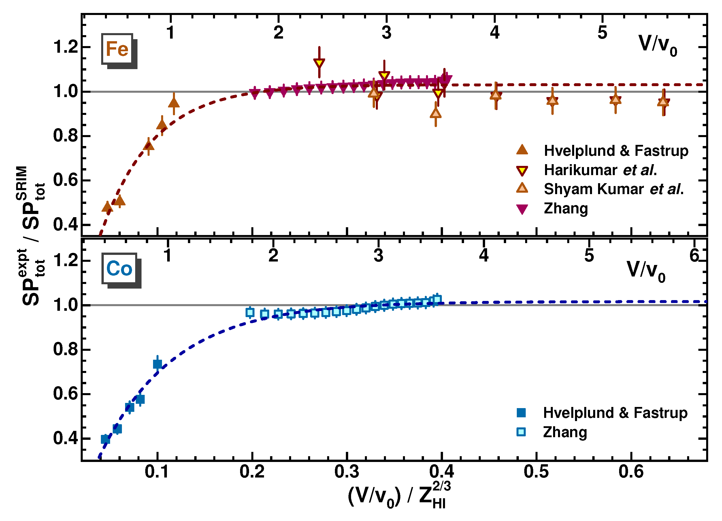
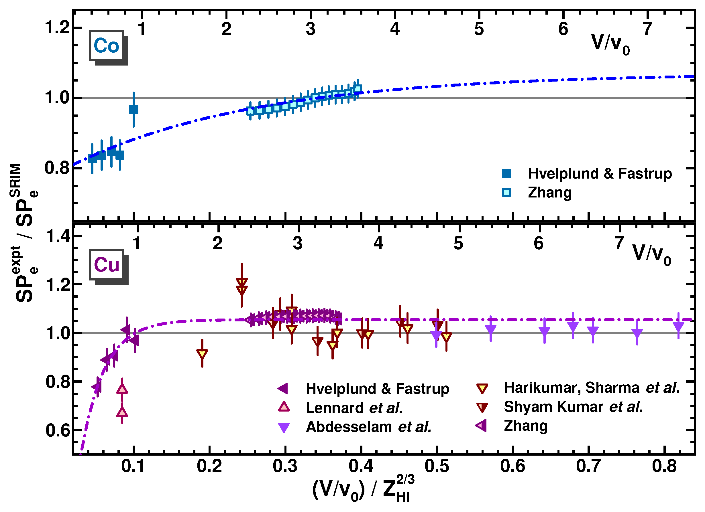
Figure 13 shows the Fe and Co SP data [7,10,32,33,35] in comparison to SRIM calculations. In contrast to the Ca and Cr data analysis (see Figure 10 and Figure 12), fitting curves provide an acceptable match of the Fe and Co data [7] (taken from the database [2]) at $V_r\gtrsim 0.2$ with the data [10] at low velocities (${\chi }_r^2=0.985$ and 0.546 were obtained for Fe and Co data fitting, respectively). The values of the fitting parameters are listed in Table 1.

Figure 13. The same as in Figure 9, Figure 10, Figure 11 and Figure 12, but for the data from [7,10,32,33,35] for Fe and Co ions (upper and bottom panels, respectively). See the text for details.

Figure 13. The same as in Figure 9, Figure 10, Figure 11 and Figure 12, but for the data from [7,10,32,33,35] for Fe and Co ions (upper and bottom panels, respectively). See the text for details.

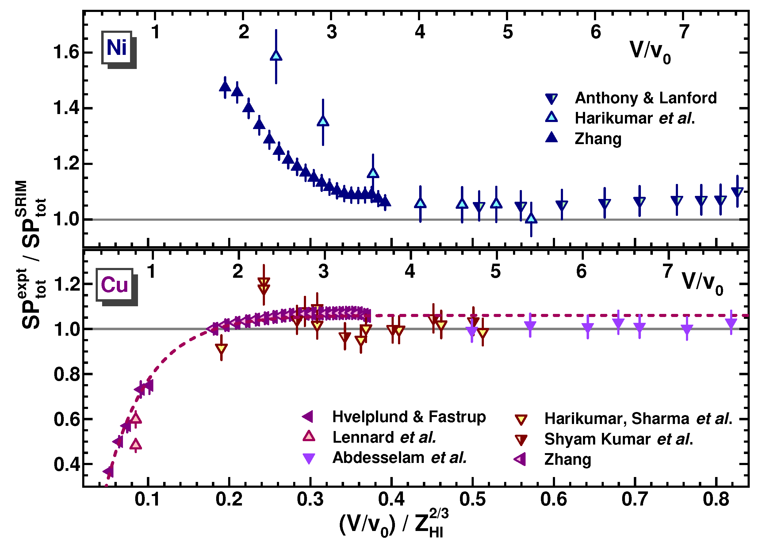
Figure 14 shows the Ni and Cu SP data [7,10,21,23,31,32,33,35] in comparison to SRIM calculations. The Ni data [21,35] at $V_r>0.4$ are in good agreement with each other and exceed SRIM calculations within ∼5%. At $V_r<0.4$, the data [7,35] significantly exceed SRIM calculations (the data [7] were taken from the database [2]). Thus, the Ni data were not processed with Equation (8). As for the Cu data, the fitting curve provides a match of the high velocity data [7,10,21,23,31,32,35] with the low-velocity ones [10]. Ignoring the data [11], ${\chi }_r^2=0.774$ was obtained. The results of the fitting are listed in Table 1.

Figure 14. The same as in Figure 9, Figure 10, Figure 11 and Figure 12, but for the data from [7,10,21,23,31,32,33,35] for Ni and Cu ions (upper and bottom panels, respectively). See the text for details.

Figure 14. The same as in Figure 9, Figure 10, Figure 11 and Figure 12, but for the data from [7,10,21,23,31,32,33,35] for Ni and Cu ions (upper and bottom panels, respectively). See the text for details.

Figure 15. The same as in Figure 9, Figure 10, Figure 11, Figure 12, Figure 13 and Figure 14, but for the data from [7,10,12,21] for Ge and Br ions (upper and bottom panels, respectively). See the text for details.

Figure 15. The same as in Figure 9, Figure 10, Figure 11, Figure 12, Figure 13 and Figure 14, but for the data from [7,10,12,21] for Ge and Br ions (upper and bottom panels, respectively). See the text for details.

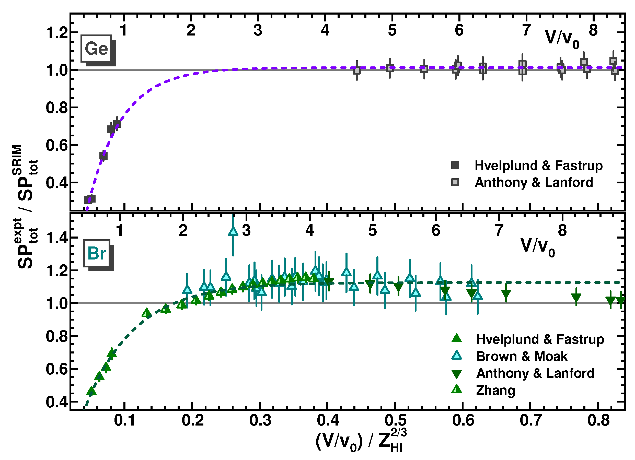
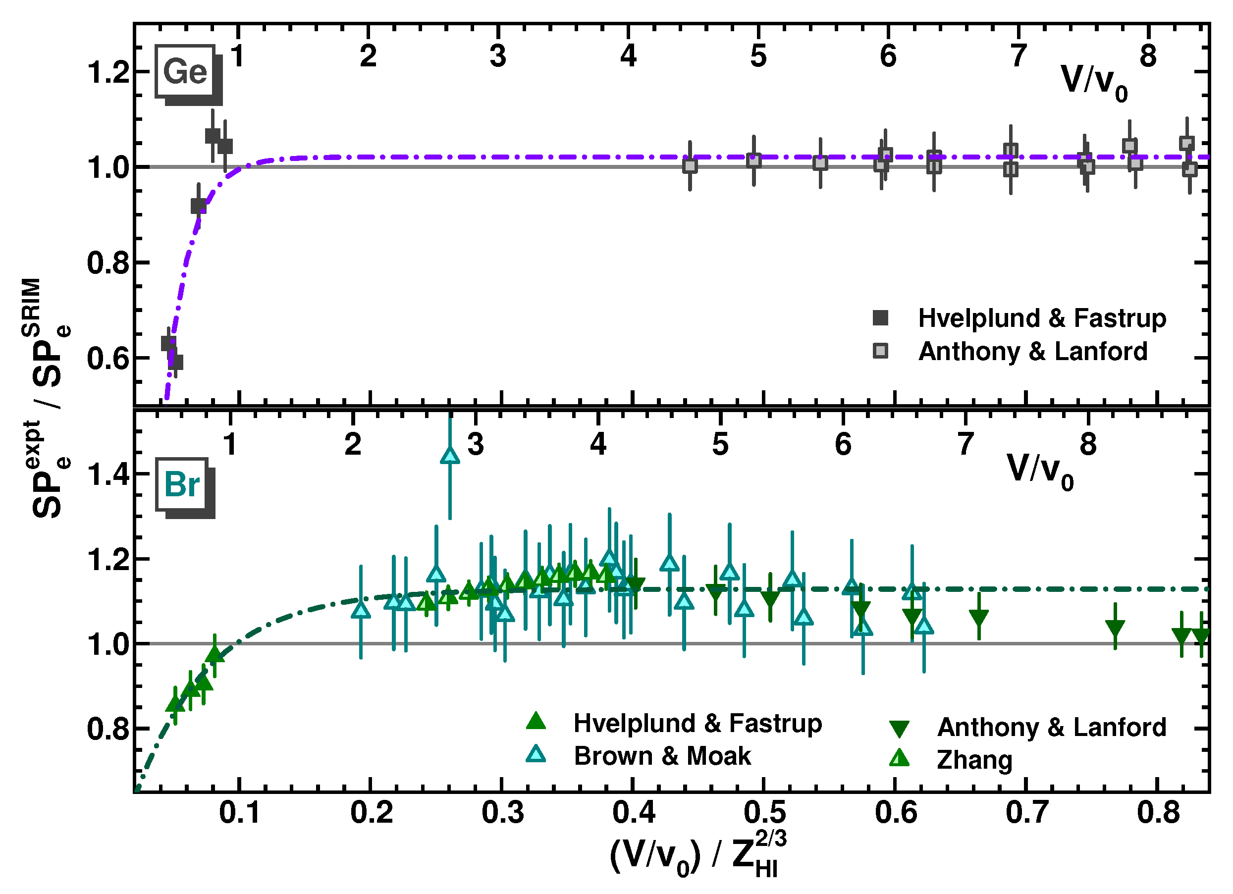
Figure 15 compares Ge and Br SP data [7,10,12,21] to SRIM calculations (the data [7] were taken from the database [2]). A lack of data for Ge ions at middle velocities ($0.1\lesssim V_r\lesssim 0.4$) makes the fitting parameters ($b_t$ and $k_t$ values) somewhat questionable, despite a good data fit (${\chi }_r^2=0.809$). The Br data [7,12,21] at $V_r\lesssim 0.6$ are reasonably consistent. The data [12] presented as the $S{P}_e$ values were corrected for $S{P}_n$. The last was calculated with an approximate expression given in reduced values [36]: $S_n\left(\epsilon \right)=0.5ln\left(1.294\epsilon \right)/\epsilon$. This correction corresponded to ≃1.5% of the $S{P}_{tot}$ value at the lowest velocities of the data [12], presented with 10% accuracy. The results of the fitting are listed in Table 1.

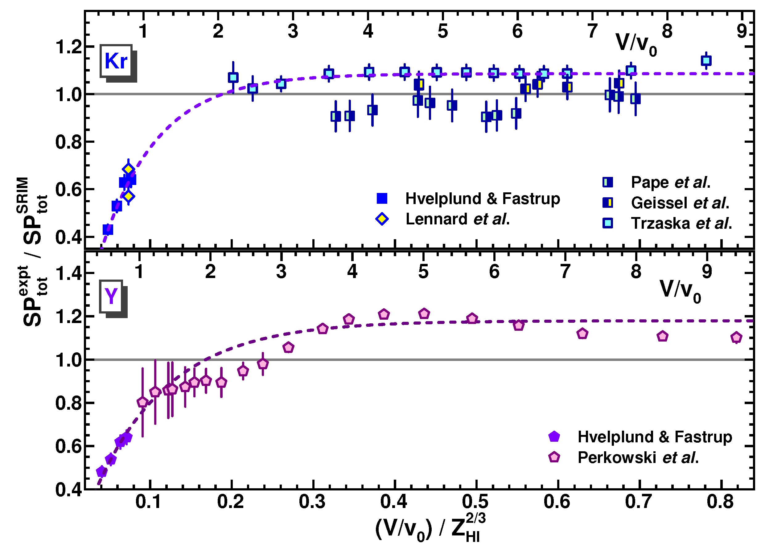
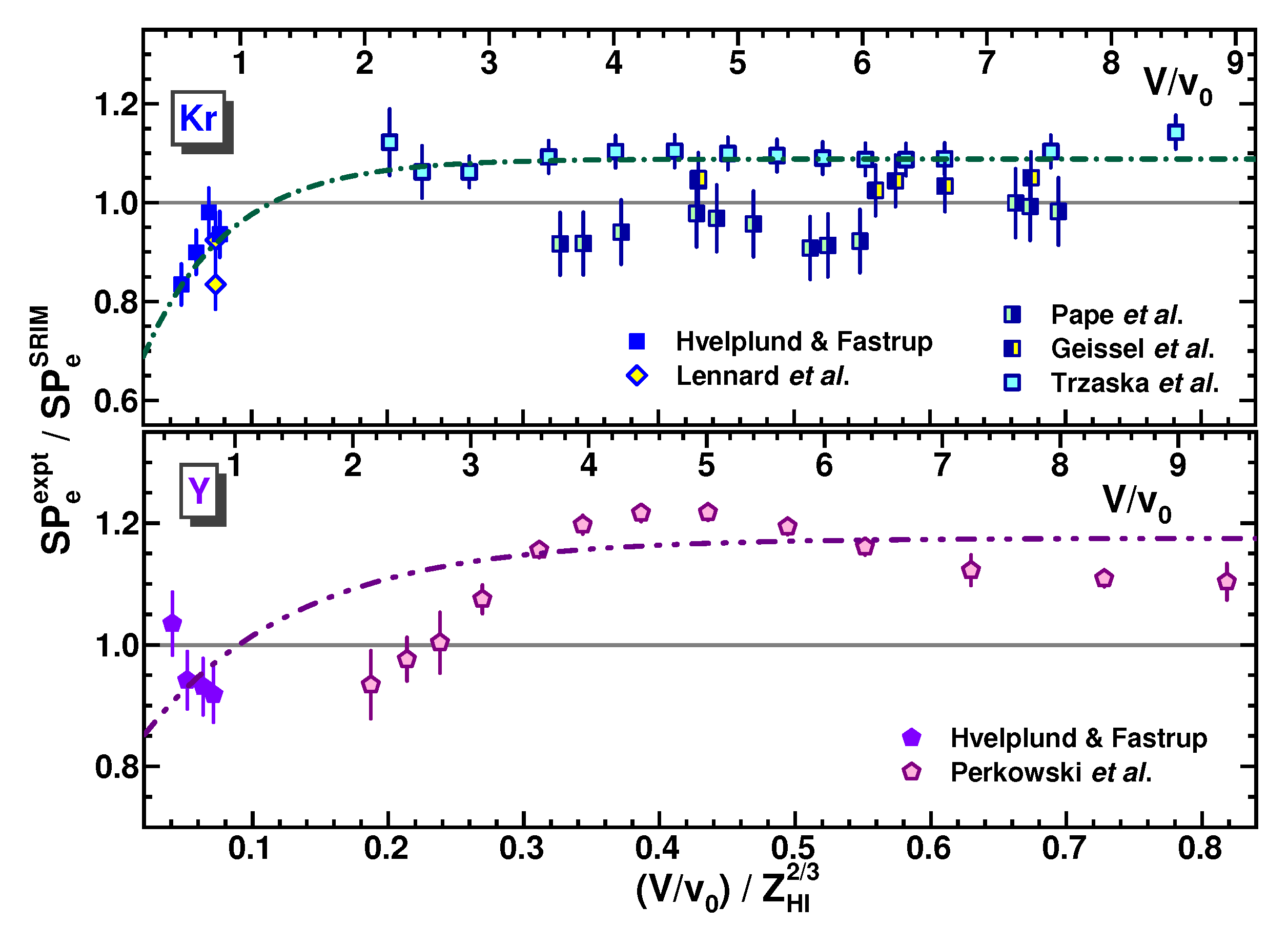
Figure 16 shows the Kr and Y SP data [10,11,20,26,28] and those obtained by Geissel et al. (taken from the database [2]) in comparison to SRIM calculations. As in the case of the Ar data, the Kr data [20] at $V_r\gtrsim 0.3$ lie noticeably below the data of Geissel et al. and the data [26], which are in satisfactory agreement with each other. The last two, together with the low-velocity data [10,11], are well fitted with Equation (8), as shown in the figure (${\chi }_r^2=0.669$). Despite well matching the Y data [28] to the low-velocity data [10], fitting yielded a large value of ${\chi }_r^2=7.38$. Implying the data [28] reliability, a bad data fit could be explained by a simplified fitting model using Equation (8), which is unable to describe the data with small errors at $0.15\lesssim V_r\lesssim 0.3$. The results of the fitting are listed in Table 1.

Figure 16. The same as in Figure 9, Figure 10, Figure 11, Figure 12, Figure 13, Figure 14 and Figure 15, but for the data from [2,10,11,20,26,28] for Kr and Y ions (upper and bottom panels, respectively). See the text for details.

Figure 16. The same as in Figure 9, Figure 10, Figure 11, Figure 12, Figure 13, Figure 14 and Figure 15, but for the data from [2,10,11,20,26,28] for Kr and Y ions (upper and bottom panels, respectively). See the text for details.

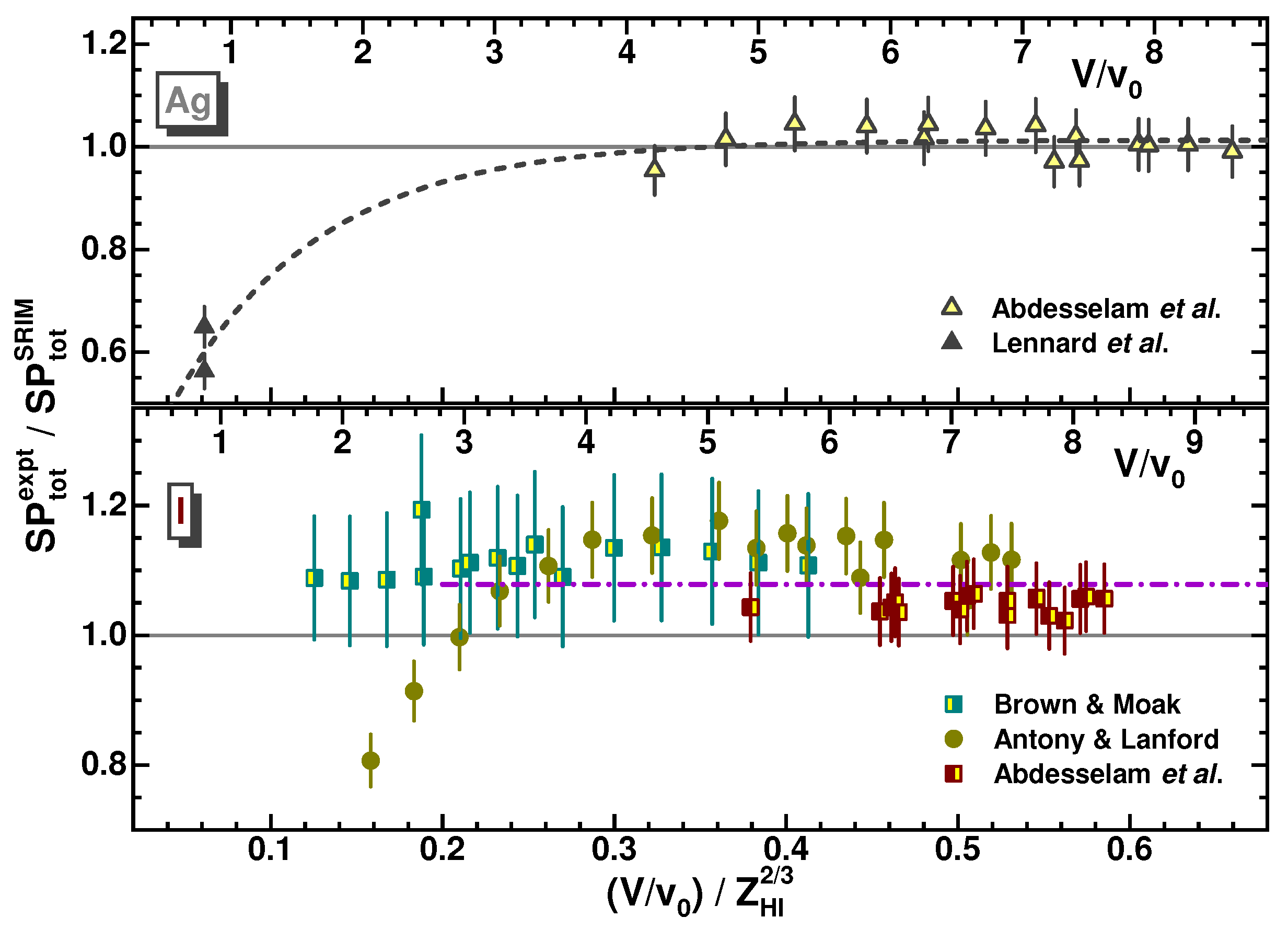
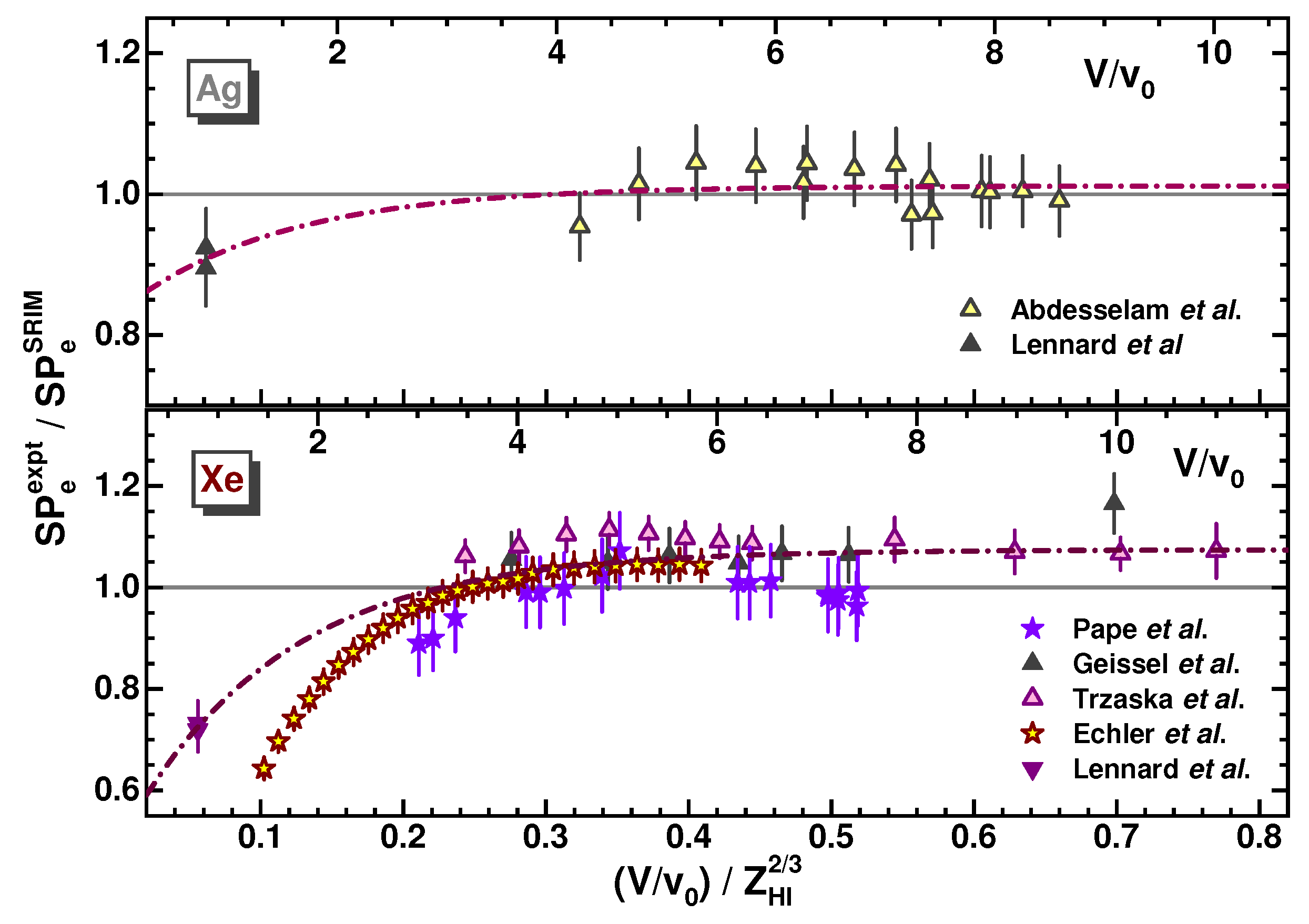
Figure 17. The same as in Figure 9, Figure 10, Figure 11, Figure 12, Figure 13, Figure 14, Figure 15 and Figure 16, but for the data from [11,12,21,23] for Ag and I ions (upper and bottom panels, respectively). See the text for details.

Figure 17. The same as in Figure 9, Figure 10, Figure 11, Figure 12, Figure 13, Figure 14, Figure 15 and Figure 16, but for the data from [11,12,21,23] for Ag and I ions (upper and bottom panels, respectively). See the text for details.

Figure 17 shows the Ag and I SP data [11,12,21,23] in comparison to SRIM calculations. The Ag data [11,23] are the only ones available. The data [23] were treated as the $S{P}_{tot}^{\mathrm{expt}}$ values because nuclear stopping contributes only 0.8% of the total stopping at the lowest velocity, according to SRIM calculations. This value is much lower than the 5% total uncertainty assigned to the data. The I data [12,21,23] at $V_r>0.2$ are quite agreeable with each other, whereas the data [12,21] are varied at $V_r<0.2$. The $S{P}_e^{\mathrm{expt}}$ data [12] were corrected for $S{P}_n$ in the same way as the Br data [12] were. Equation (8) was used to fit the Ag data, whereas the I data at $V_r>0.2$ could be fitted with a constant for the $S{P}_{tot}^{\mathrm{expt}}/S{P}_{tot}^{\mathrm{SRIM}}$ ratios, as was performed for the V data (see Figure 11).

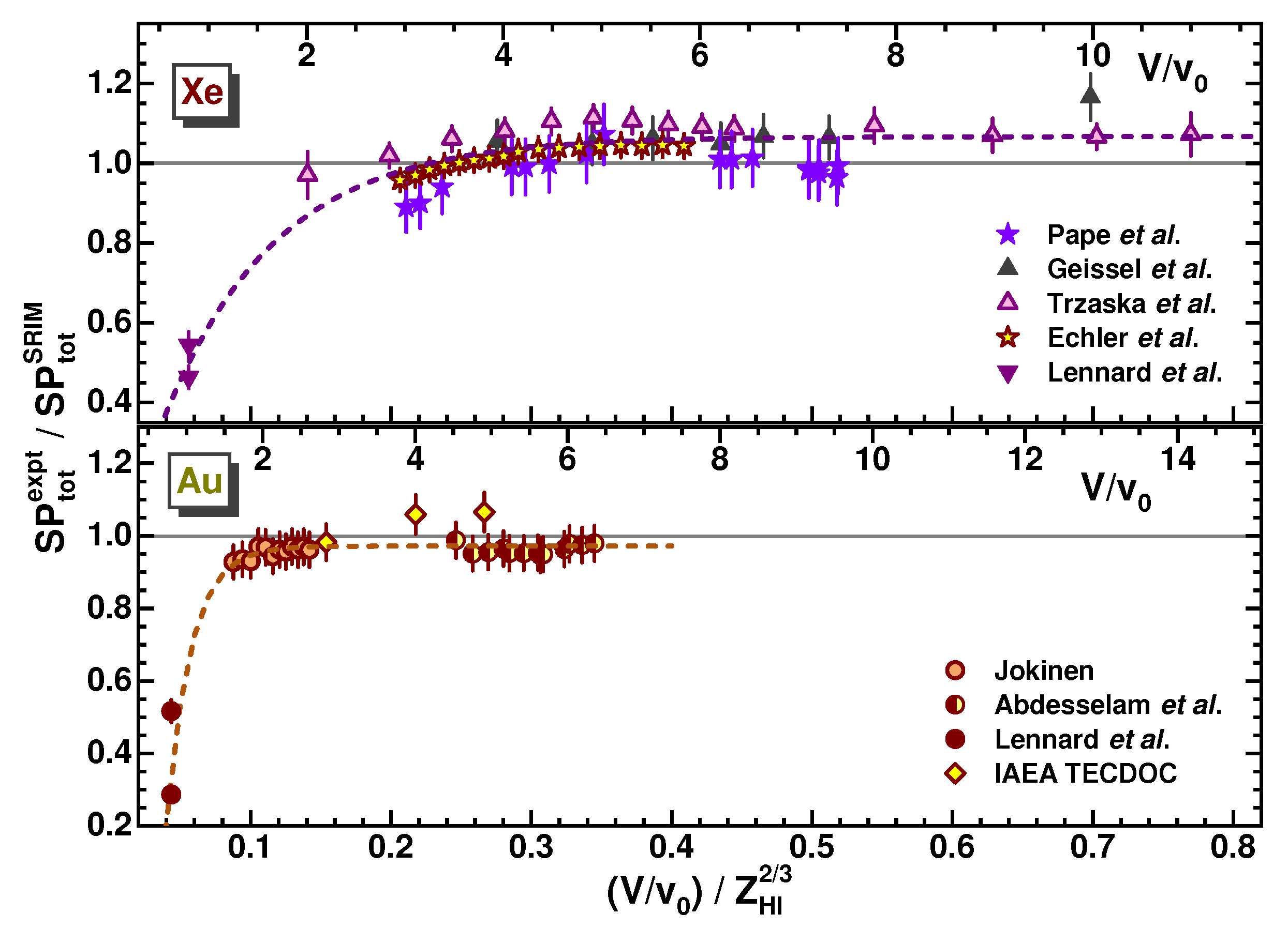
Figure 18 shows the Xe and Au SP data [11,20,23,26,29,37], which are compared to SRIM calculations. The data obtained by Geissel et al. for Xe, and those indicated as IAEA TECDOC for Au were taken from the database [2]. The Xe data at $0.2<V_r<0.6$ are close to each other. The data [37] originally presented as $S{P}_e^{\mathrm{expt}}$ were limited to $V_r\gtrsim 0.2$. At these velocities, $S{P}_n^{\mathrm{SRIM}}$ values contribute less than 3% of $S{P}_{tot}^{\mathrm{SRIM}}$, which is less than the respective data errors assigned in [37]. The Au data [23] were assigned to the $S{P}_{tot}^{\mathrm{expt}}$ values because nuclear stopping contributes only 1.5% of total stopping at the lowest energy, according to SRIM calculations. That is much less than the respective errors assigned in the work. For the Au data [29], $S{P}_{tot}^{\mathrm{expt}}=\Delta E/\Delta X$ estimates were based on the tabulated $\Delta E$ data. These data corresponded to the Au input energies, $E_{in}$ = 15–37 MeV. The average energies for the $S{P}_{tot}^{\mathrm{expt}}$ values thus obtained corresponded to $E_{av}=E_{in}-S{P}_{tot}^{\mathrm{expt}}\Delta X/2$. The Xe and Au data [11] at $0.8v_0$, corresponding to the different target thicknesses, were added, and both the data sets were fitted with Equation (8). The steep fall from the Au SP data [23,29] to those obtained at $0.8v_0$ [11] led to the large $b_t$ and $k_t$ fitted values (obtained with large errors), which noticeably exceeded those for other HIs (see Table 1).

Figure 18. The same as in Figure 9, Figure 10, Figure 11, Figure 12, Figure 13, Figure 14, Figure 15, Figure 16 and Figure 17, but for the data from [11,20,23,26,29,37] for Xe and Au ions (upper and bottom panels, respectively). See the text for details.

Figure 18. The same as in Figure 9, Figure 10, Figure 11, Figure 12, Figure 13, Figure 14, Figure 15, Figure 16 and Figure 17, but for the data from [11,20,23,26,29,37] for Xe and Au ions (upper and bottom panels, respectively). See the text for details.

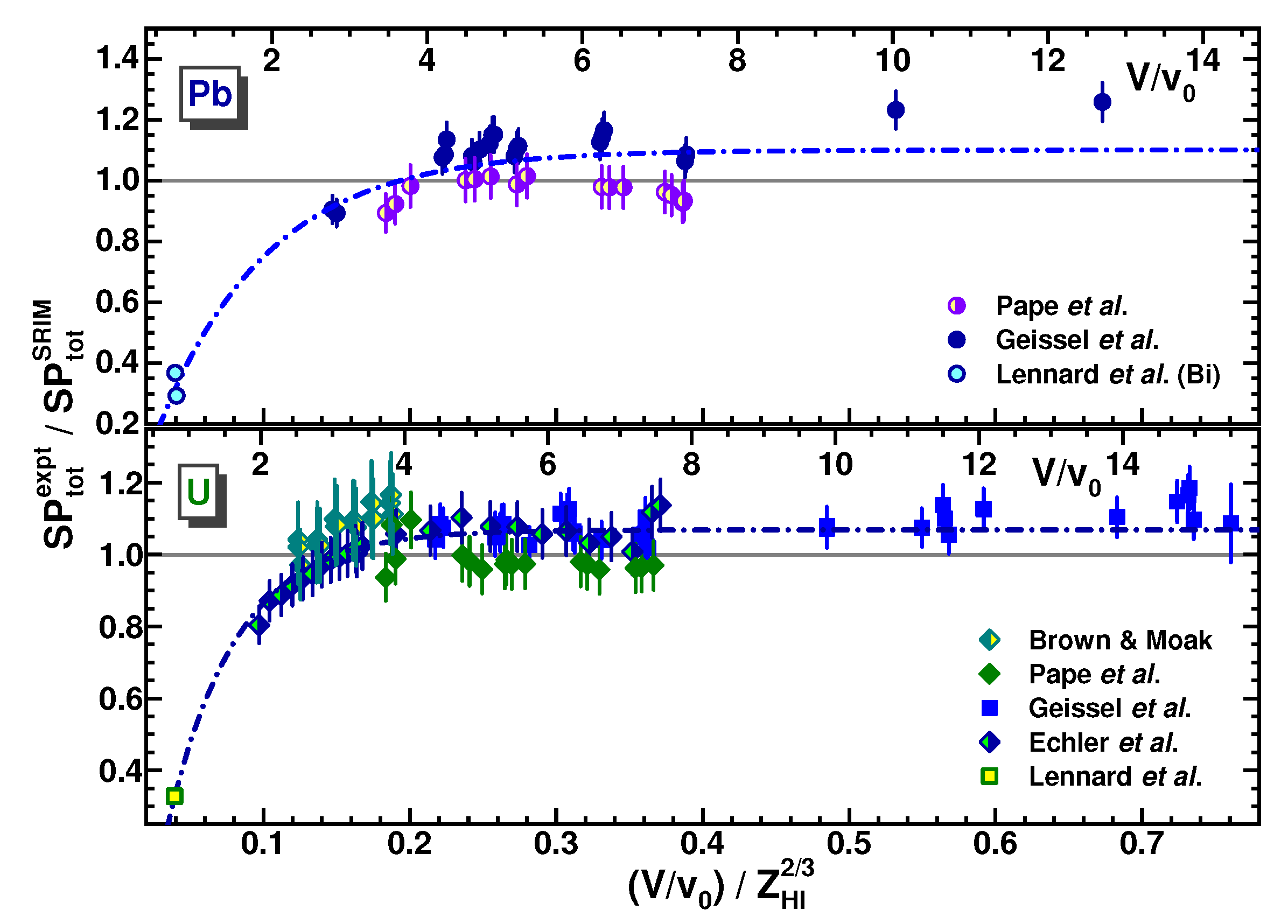
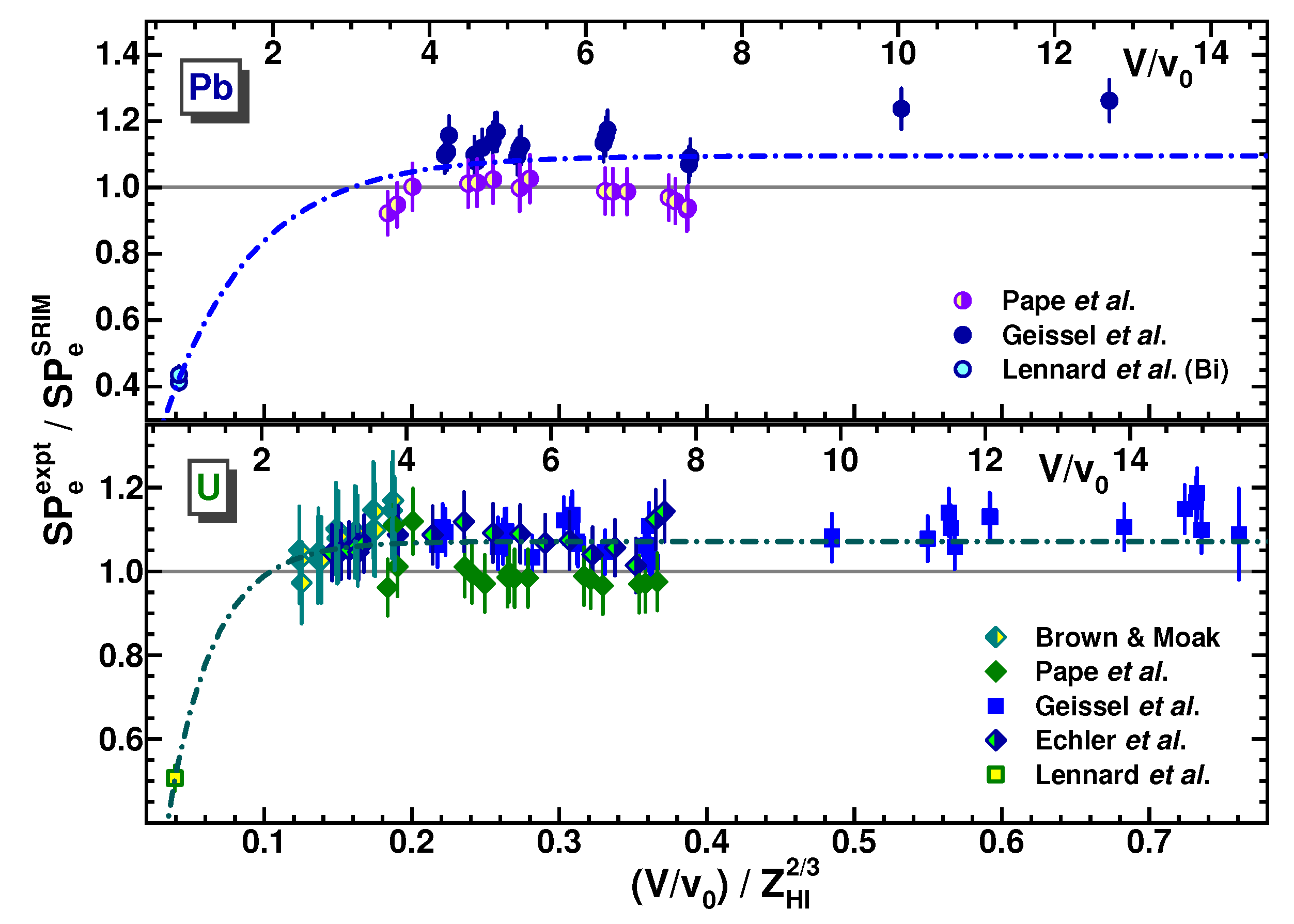
Figure 19 shows the Pb and U SP data [11,12,20,30], and those obtained by Geissel et al. (taken from the database [2]) in comparison to SRIM calculations. Though the Pb data [20] and those of Geissel et al. are in some disagreement with each other, they were fitted together with Equation (8). A similar difference is seen for the U data of the same authors. These data, together with others [12,30], are in satisfactory agreement with each other. The U data [12] presented as the $S{P}_e$ values were corrected for $S{P}_n$ in the same way as was performed for the Br and I data [12]. The resulting $S{P}_{tot}^{\mathrm{expt}}$ data are slightly higher than the data [30] obtained later at the same velocities, but they are consistent within the error bars with the rest of the data, as seen in the figure. The Pb and U data were supplemented with the low-velocity Bi and U data [11]. In doing so, a possible distinction in the SP values for Pb and Bi were neglected. The results of fitting are listed in Table 1.

Figure 19. The same as in Figure 9, Figure 10, Figure 11, Figure 12, Figure 13, Figure 14, Figure 15, Figure 16, Figure 17 and Figure 18, but for the data from [2,11,12,20,30] for Pb and U ions only (upper and bottom panels, respectively). See the text for details.

Figure 19. The same as in Figure 9, Figure 10, Figure 11, Figure 12, Figure 13, Figure 14, Figure 15, Figure 16, Figure 17 and Figure 18, but for the data from [2,11,12,20,30] for Pb and U ions only (upper and bottom panels, respectively). See the text for details.

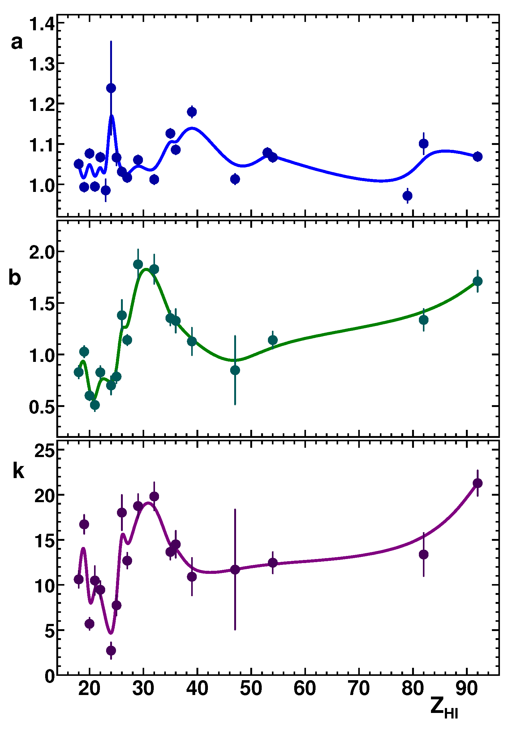
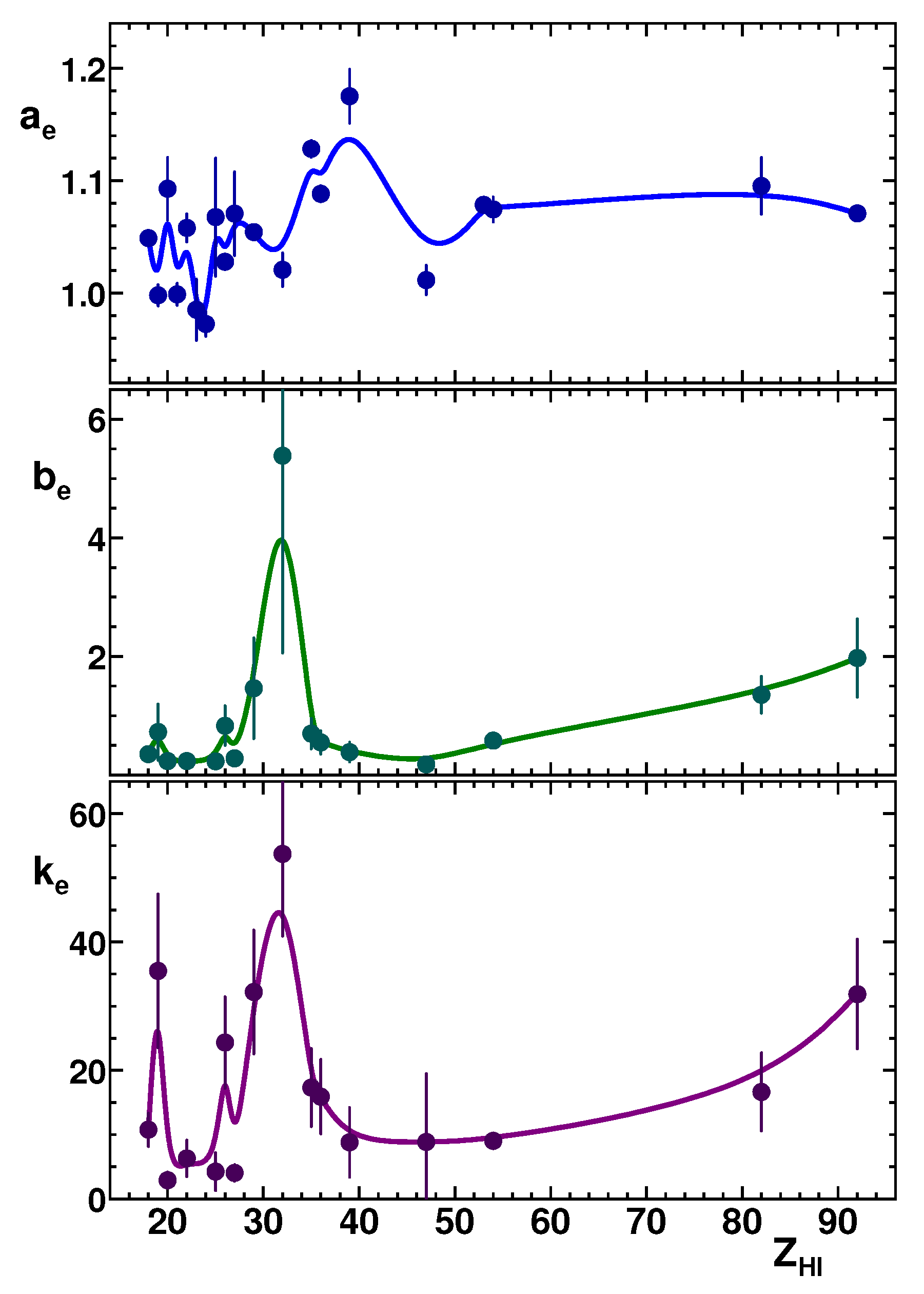
In Figure 20, the fitting parameters listed in Table 1 are shown as a function of the HI atomic number. As one can see in the figure, an amplitude $a_t$, corresponding to the ratio of $S{P}_{tot}^{\mathrm{expt}}/S{P}_{tot}^{\mathrm{SRIM}}$ at high velocities, oscillates in a sporadic way within a magnitude range of 0.9–1.2. The exponent parameters ($b_t$ and $k_t$), which determine decreasing $S{P}_{tot}^{\mathrm{expt}}/S{P}_{tot}^{\mathrm{SRIM}}$ ratios at low velocities, correlate with each other to a certain extent in the region of $24\lesssim Z_{\mathrm{HI}}\lesssim 40$ and, probably, for higher $Z_{\mathrm{HI}}$ (the Au parameters have been omitted from the consideration due to their enormous large values and errors). The parameterization with Equation (8) using the parameter values listed in Table 1 (along with their interpolation for $Z_{\mathrm{HI}}$ not listed in the table) seems to be useful for the estimates of the total carbon SP at low velocities, which can be applied as the correction to the SRIM calculations.

Figure 20. Fitting parameters $a_t$, $b_t$, and $k_t$ listed in Table 1 are shown as functions of the HI atomic number (from upper to bottom panels, respectively). Solid lines are B-spline approximations.

Figure 20. Fitting parameters $a_t$, $b_t$, and $k_t$ listed in Table 1 are shown as functions of the HI atomic number (from upper to bottom panels, respectively). Solid lines are B-spline approximations.

Now, using Equations (1) and (8) with the parameter values listed in Table 1, one could estimate the $S{P}_n^{\mathrm{expt}}$ values as

$$S{P}_n^{\mathrm{expt}}=f_{tot}^{cor}\left(V_r\right)S{P}_{tot}^{\mathrm{SRIM}}-S{P}_e^{\mathrm{expt}},$$

(10)

where $S{P}_e^{\mathrm{expt}}$ is the electronic SP obtained in experiments. The $S{P}_e^{\mathrm{expt}}$ estimates are considered in the next section. An approximation similar to Equation (8) can be applied to the available $S{P}_e^{\mathrm{expt}}$ data, assuming their reliability, together with $S{P}_e^{\mathrm{SRIM}}$ calculations. This reasoning takes into consideration that relatively small values of $S{P}_n$ were subtracted from $S{P}_{tot}^{\mathrm{expt}}$ in order to obtain $S{P}_e^{\mathrm{expt}}$ in the low-velocity experiments [9,10,11], whereas at relatively high velocities, $S{P}_e^{\mathrm{expt}}$ values do not differ from $S{P}_{tot}^{\mathrm{expt}}$ ones with a good degree of accuracy. The inspection of the low-velocity data [9,10] showed that the contribution of the estimated $S{P}_n$ values does not exceed 25% as a whole (the only exception is about 29% for Fe at the lowest energy). This is the case for the energy-loss thin target data [11], whereas for the thick target data [11] for Xe and heavier ions, this contribution exceeds 29%.

3.2. Electronic Stopping Power Data Analysis

In Figure 21, Figure 22, Figure 23, Figure 24, Figure 25, Figure 26, Figure 27, Figure 28 and Figure 29, electronic SP values derived from experiments for Ar to U ions are compared with those obtained with SRIM calculations. Some details about the $S{P}_e^{\mathrm{expt}}$ data used within this consideration should be mentioned, and they are discussed below. As with the $S{P}_{tot}^{\mathrm{expt}}$, the analysis favored the use of the available original data (with the original errors). The $S{P}_e^{\mathrm{expt}}/S{P}_e^{\mathrm{SRIM}}$ values were fitted using the weighted LSM procedure with the exponential correction function of $V_r$, similar to Equation (8):

$$f_{el}^{cor}\left(V_r\right)=S{P}_e^{\mathrm{expt}}/S{P}_e^{\mathrm{SRIM}}=a_e-b_{e}exp(-k_e{V}_r),$$

(11)

where $a_e$, $b_e$, and $k_e$ are fitting parameters.

The ratios of the $S{P}_e^{\mathrm{expt}}$ and $S{P}_e^{\mathrm{SRIM}}$ values for Ar and K ions are shown in Figure 21. The Ar and K $S{P}_e^{\mathrm{expt}}$ data [9,11,20,22,26,31] were taken from the works’ respective tables, whereas the Ar data of Geissel et al. were from the database [2]. High velocity data [20,31] and those of Geissel et al. are the same as shown in Figure 9, whereas the data [26] are limited to velocities $V_r>0.3$. The limit corresponds to the value from which $S{P}_n^{\mathrm{SRIM}}$ gives a lower contribution than the SP data errors assigned in [26]. The Ar data [20] are in contrast to similar ones [26] and those of Geissel et al., which are in agreement with each other. The low-velocity data [11] also contradict the data [9,22], as shown in Figure 21. As a result, the data [11,20] were removed from the fitting of the $S{P}_e^{\mathrm{expt}}/S{P}_e^{\mathrm{SRIM}}$ ratio. The fitting parameter values thus obtained for the Ar and K data are listed in Table 2.

Figure 22 shows the Ca and Sc electronic SP data [9,10,11,26,27,31,32] in comparison to the SRIM calculations. As in Figure 10, the fitting curve does not provide Ca data for the match with Equation (11) even after omitting the data [31] at $0.3<V_r<0.4$. Note that the $S{P}_n^{\mathrm{SRIM}}$ value at the lowest $V_r$ of the data [27] corresponds to 2% of $S{P}_{tot}^{\mathrm{SRIM}}$, which is smaller than the SP data error (3.8%) assigned in the work. Thus, the data [27] could be related to $S{P}_e^{\mathrm{expt}}$ values within the whole range of $V_r$. It is implied that the electronic SP data [27] at relatively high velocities and the data [9] at relatively low velocities are reliable, as for the total SP considerations. The best Sc data fit was obtained with a constant SP ratio when the data [11] were ignored. The latter correspond to noticeably lower electronic SP values than those obtained in [9]. The results of the Ca and Sc data fitting are listed in Table 2.

Figure 21. $S{P}_e^{\mathrm{expt}}/S{P}_e^{\mathrm{SRIM}}$ ratios for Ar and K data, [9,11,20,22,26,31] and Ar data [2] of Geissel et al. (upper and bottom panels, respectively). The results of the data fitting with Equation (11) are shown by dash-dotted lines (the data [11,20] were excluded). The upper axes of the panels correspond to relative velocity $V/v_0$, shown for orientation. See the text for details.

Figure 21. $S{P}_e^{\mathrm{expt}}/S{P}_e^{\mathrm{SRIM}}$ ratios for Ar and K data, [9,11,20,22,26,31] and Ar data [2] of Geissel et al. (upper and bottom panels, respectively). The results of the data fitting with Equation (11) are shown by dash-dotted lines (the data [11,20] were excluded). The upper axes of the panels correspond to relative velocity $V/v_0$, shown for orientation. See the text for details.

Figure 22. The same as in Figure 21, but for the data from [9,10,11,26,27,31,32] for Ca and Sc ions (upper and bottom panels, respectively). See the text for details.

Figure 22. The same as in Figure 21, but for the data from [9,10,11,26,27,31,32] for Ca and Sc ions (upper and bottom panels, respectively). See the text for details.

Figure 23 shows the Ti and Cr electronic SP data [7,10,11,20,21,23,31,32,33], together with the Ti data of Geissel et al. in comparison to SRIM calculations. The Ti data [21] and those of Geissel et al., as well as Cr data [7] were taken from the database [2]. The Ti data at relatively high velocities ($V_r\gtrsim 0.3$) are in satisfactory agreement with each other. The Cr data [7] at the lowest velocities, for which the $S{P}_n^{\mathrm{SRIM}}$ values exceeded data errors (2.5%), were excluded from fitting. The best Cr data fit was obtained with a constant SP ratio, when the datum [11] was disregarded. The last corresponds to the significantly lower electronic SP value than the one obtained in [9] at the same velocity. The results of the data fitting are given in Table 2.

Figure 24 compares the Mn and Fe electronic SP data [7,10,11,31,32,33,35] to SRIM calculations (the data [7] were taken from the database [2]). The Mn data [31,32] at $0.2\lesssim V_r\lesssim 0.5$ differ from the data [7] obtained later with minor errors. The Mn datum [11] at $0.8v_0$ does not agree with the data [10] at the same velocity and was excluded from fitting. The Mn and Fe data [7] at the lowest velocities, for which the $S{P}_n^{\mathrm{SRIM}}$ values exceeded data errors (2.5%), were also excluded from fitting. The results of the fitting are listed in Table 2.

Figure 23. The same as in Figure 21 and Figure 22, but for the data from [7,10,11,20,21,23,31,32,33] for Ti and Cr ions (upper and bottom panels, respectively). See the text for details.

Figure 23. The same as in Figure 21 and Figure 22, but for the data from [7,10,11,20,21,23,31,32,33] for Ti and Cr ions (upper and bottom panels, respectively). See the text for details.

Figure 24. The same as in Figure 21, Figure 22 and Figure 23, but for the data from [7,10,11,31,32,33,35] for Mn and Fe ions (upper and bottom panels, respectively). See the text for details.

Figure 24. The same as in Figure 21, Figure 22 and Figure 23, but for the data from [7,10,11,31,32,33,35] for Mn and Fe ions (upper and bottom panels, respectively). See the text for details.

Figure 25 compares the Co and Cu electronic SP data [7,10,11,23,32,33,35] to the SRIM calculations (the data [7] were taken from the database [2]). The SP data [7] at the lowest velocities, at which the $S{P}_n^{\mathrm{SRIM}}$ values exceeded the data errors (2.5%), were excluded from fitting. The Cu data [11] at $0.8v_0$ contradicted the data [10] at the same velocity and were excluded from fitting. As a result, the fitting curves provide rather good matches for the Co and Cu data [7] with the data [10] obtained at low velocities. At the same time, these curves vary markedly. The results of the fitting are listed in Table 2.

Figure 26 compares the Ge and Br electronic SP data [7,10,12,21] to the SRIM calculations (the data [7] were taken from the database [2]). The Br data [7,12,21] at $V_r\lesssim 0.6$ are reasonably consistent. As in previous cases, the Br data [7] at the lowest velocities, for which the $S{P}_n^{\mathrm{SRIM}}$ values exceeded the data errors (2.5%), were excluded from fitting. As in the case of the Co and Cu ratios, fitting curves obtained for the Ge and Br ratios vary markedly. The results of the fitting are listed in Table 2.

Figure 25. The same as in Figure 21, Figure 22, Figure 23 and Figure 24, but for the data from [7,10,11,23,32,33,35] for Co and Cu ions (upper and bottom panels, respectively). See the text for details.

Figure 25. The same as in Figure 21, Figure 22, Figure 23 and Figure 24, but for the data from [7,10,11,23,32,33,35] for Co and Cu ions (upper and bottom panels, respectively). See the text for details.

Figure 26. The same as in Figure 21, Figure 22, Figure 23, Figure 24 and Figure 25, but for the data from [7,10,12,21] for Ge and Br ions (upper and bottom panels, respectively). See the text for details.

Figure 26. The same as in Figure 21, Figure 22, Figure 23, Figure 24 and Figure 25, but for the data from [7,10,12,21] for Ge and Br ions (upper and bottom panels, respectively). See the text for details.

Figure 27 shows the Kr and Y electronic SP data and those obtained by Geissel et al. (taken from the database [2]) in comparison to the SRIM calculations. As for the Ar data, the Kr data [20] at $V_r\gtrsim 0.3$ lie noticeably below the data of Geissel et al. and the data [26], which are in satisfactory agreement with each other. Note that the errors in the Kr data [26] at the lowest velocities exceed the respective $S{P}_n^{\mathrm{SRIM}}$ values. The data [26], together with the data of Geissel et al. and the low-velocity data [10,11], are well fitted with Equation (11), as shown in the figure. Fitting the Y data was restricted by the velocities at which the $S{P}_n^{\mathrm{SRIM}}$ values did not exceed data errors when the data [28] are considered. These data do not match the low-velocity data [10] (${\chi }_r^2=8.50$ was obtained using Equation (11)) Implying the reliability of the data [28], a bad data fit could be explained by the oversimplified fitting model, which cannot describe the specific behavior of the SP ratios obtained with these data in contrast to the others considered here. The results of the fitting are listed in Table 2.

Figure 27. The same as in Figure 21, Figure 22, Figure 23, Figure 24, Figure 25 and Figure 26, but for the data from [2,10,11,20,26,28] for Kr and Y ions (upper and bottom panels, respectively). See the text for details.

Figure 27. The same as in Figure 21, Figure 22, Figure 23, Figure 24, Figure 25 and Figure 26, but for the data from [2,10,11,20,26,28] for Kr and Y ions (upper and bottom panels, respectively). See the text for details.

Table 2. Fitting parameter values $a_e$, $b_e$, and $k_e$, as obtained for the Ar to U $S{P}_e^{\mathrm{expt}}/S{P}_e^{\mathrm{SRIM}}$ data fitted with Equation (11). The ion symbols and ranges of the applicability of Equation (11) for specified ions are listed in the first and last columns, respectively. The results of data fitting are shown in Figure 21, Figure 22, Figure 23, Figure 24, Figure 25, Figure 26, Figure 27, Figure 28 and Figure 29.

Ion	${\mathit{a}}_{\mathit{e}}$	${\mathit{b}}_{\mathit{e}}$	${\mathit{k}}_{\mathit{e}}$	${\mathit{V}}_{\mathit{r}}$ Range
Ar 1	$1.0490\pm 0.0056$	$0.351\pm 0.076$	$10.8\pm 2.6$	0.05–0.8
K 2	$0.9980\pm 0.0095$	$0.725\pm 0.474$	$35.5\pm 12.0$	0.05–0.6
Ca 3	$1.0928\pm 0.0279$	$0.236\pm 0.043$	$2.92\pm 1.27$	0.06–0.9
Sc 2	$0.9989\pm 0.0098$			0.06–0.8
Ti	$1.0580\pm 0.0126$	$0.233\pm 0.057$	$6.29\pm 2.85$	0.06–0.8
V	$0.9852\pm 0.0274$			0.2–0.6
Cr 2,4	$0.9725\pm 0.0110$			0.06–0.7
Mn 2,4	$1.0676\pm 0.0526$	$0.231\pm 0.053$	$4.3\pm 3.0$	0.06–0.7
Fe 4	$1.0278\pm 0.0054$	$0.832\pm 0.335$	$24.3\pm 7.1$	0.04–0.7
Co 4	$1.0707\pm 0.0373$	$0.282\pm 0.027$	$4.04\pm 1.29$	0.04–0.5
Cu 2,4	$1.0542\pm 0.0055$	$1.464\pm 0.849$	$32.2\pm 9.6$	0.05–0.8
Ge	$1.0207\pm 0.0150$	$5.385\pm 3.329$	$53.7\pm 12.8$	0.04–0.9
Br	$1.1284\pm 0.0075$	$0.697\pm 0.256$	$17.3\pm 6.1$	0.04–0.9
Kr 5	$1.0883\pm 0.0072$	$0.550\pm 0.197$	$15.9\pm 5.8$	0.04–0.8
Y	$1.1752\pm 0.0239$	$0.386\pm 0.166$	$8.8\pm 5.4$	0.04–0.8
Ag	$1.0116\pm 0.0131$	$0.178\pm 0.110$	$8.9\pm 10.7$	0.06–0.7
I	$1.0786\pm 0.0069$			0.2–0.6
Xe	$1.0744\pm 0.0111$	$0.579\pm 0.065$	$9.03\pm 1.23$	0.05–0.8
Pb	$1.0953\pm 0.0252$	$1.352\pm 0.313$	$16.7\pm 6.1$	0.04–0.8
U	$1.0709\pm 0.0061$	$1.972\pm 0.661$	$31.9\pm 8.5$	0.04–0.8

¹ Without the data [11,20] (see the text). ² Without the data [11] (see the text). ³ Without the data [31] at $0.3<V_r<0.4$ (see the text). ⁴ Without the data [7] at the lowest velocities (see the text). ⁵ Without the data [20] (see the text).

Table 2. Fitting parameter values $a_e$, $b_e$, and $k_e$, as obtained for the Ar to U $S{P}_e^{\mathrm{expt}}/S{P}_e^{\mathrm{SRIM}}$ data fitted with Equation (11). The ion symbols and ranges of the applicability of Equation (11) for specified ions are listed in the first and last columns, respectively. The results of data fitting are shown in Figure 21, Figure 22, Figure 23, Figure 24, Figure 25, Figure 26, Figure 27, Figure 28 and Figure 29.

Ion	${\mathit{a}}_{\mathit{e}}$	${\mathit{b}}_{\mathit{e}}$	${\mathit{k}}_{\mathit{e}}$	${\mathit{V}}_{\mathit{r}}$ Range
Ar 1	$1.0490\pm 0.0056$	$0.351\pm 0.076$	$10.8\pm 2.6$	0.05–0.8
K 2	$0.9980\pm 0.0095$	$0.725\pm 0.474$	$35.5\pm 12.0$	0.05–0.6
Ca 3	$1.0928\pm 0.0279$	$0.236\pm 0.043$	$2.92\pm 1.27$	0.06–0.9
Sc 2	$0.9989\pm 0.0098$			0.06–0.8
Ti	$1.0580\pm 0.0126$	$0.233\pm 0.057$	$6.29\pm 2.85$	0.06–0.8
V	$0.9852\pm 0.0274$			0.2–0.6
Cr 2,4	$0.9725\pm 0.0110$			0.06–0.7
Mn 2,4	$1.0676\pm 0.0526$	$0.231\pm 0.053$	$4.3\pm 3.0$	0.06–0.7
Fe 4	$1.0278\pm 0.0054$	$0.832\pm 0.335$	$24.3\pm 7.1$	0.04–0.7
Co 4	$1.0707\pm 0.0373$	$0.282\pm 0.027$	$4.04\pm 1.29$	0.04–0.5
Cu 2,4	$1.0542\pm 0.0055$	$1.464\pm 0.849$	$32.2\pm 9.6$	0.05–0.8
Ge	$1.0207\pm 0.0150$	$5.385\pm 3.329$	$53.7\pm 12.8$	0.04–0.9
Br	$1.1284\pm 0.0075$	$0.697\pm 0.256$	$17.3\pm 6.1$	0.04–0.9
Kr 5	$1.0883\pm 0.0072$	$0.550\pm 0.197$	$15.9\pm 5.8$	0.04–0.8
Y	$1.1752\pm 0.0239$	$0.386\pm 0.166$	$8.8\pm 5.4$	0.04–0.8
Ag	$1.0116\pm 0.0131$	$0.178\pm 0.110$	$8.9\pm 10.7$	0.06–0.7
I	$1.0786\pm 0.0069$			0.2–0.6
Xe	$1.0744\pm 0.0111$	$0.579\pm 0.065$	$9.03\pm 1.23$	0.05–0.8
Pb	$1.0953\pm 0.0252$	$1.352\pm 0.313$	$16.7\pm 6.1$	0.04–0.8
U	$1.0709\pm 0.0061$	$1.972\pm 0.661$	$31.9\pm 8.5$	0.04–0.8

¹ Without the data [11,20] (see the text). ² Without the data [11] (see the text). ³ Without the data [31] at $0.3<V_r<0.4$ (see the text). ⁴ Without the data [7] at the lowest velocities (see the text). ⁵ Without the data [20] (see the text).

The iodine stopping power data [12,21,23] at $V_r>0.2$ (considered in Section 3.1) are in rather good agreement with each other, whereas at $V_r<0.2$, the data [12,21] are varied (see Figure 17). At $V_r>0.2$, the $S{P}_n^{\mathrm{SRIM}}$ values are less than 3% of $S{P}_{tot}^{\mathrm{SRIM}}$ and less than the data errors (5–10%). Thus, the electronic SP ratios at $V_r>0.2$ for I ions are the same as the ones obtained by a constant fit to the iodine $S{P}_{tot}^{\mathrm{expt}}/S{P}_{tot}^{\mathrm{SRIM}}$ ratios (see Table 2).

Figure 28 shows the Ag and Xe electronic SP data [11,12,20,21,23,26,37], and those obtained by Geissel et al. (taken from the database [2]) in comparison to SRIM calculations. For the Ag data [23] at the lowest velocity, nuclear stopping accounts for 0.8% of total stopping (which is much lower than the 5% uncertainty assigned to the data). These data were attributed to the $S{P}_e^{\mathrm{expt}}$ ones. The Xe data [26] at the lowest velocities, for which the $S{P}_n^{\mathrm{SRIM}}$ values exceeded the data errors, were excluded from fitting. The original $S{P}_e^{\mathrm{expt}}$ data [37] at $V_r\gtrsim 0.2$ were only used for Xe data fitting. At these velocities, $S{P}_n^{\mathrm{SRIM}}$ values contribute less than 3% of $S{P}_{tot}^{\mathrm{SRIM}}$ (which is less than the respective data errors assigned in [37]). TRIM simulations were used for the estimates of the $S{P}_n$ values in [37], with their subsequent subtraction from the measured $S{P}_{tot}^{\mathrm{expt}}$. The low-velocity data [37] at $V_r\lesssim 0.2$, shown in the figure, disagree with the data [11] due to the overestimation of nuclear stopping in the TRIM simulations. At the same time, all the Xe data at $V_r>0.2$ are in satisfactory agreement with each other. The results of the fitting with Equation (11) are listed in Table 2.

Figure 28. The same as in Figure 21, Figure 22, Figure 23, Figure 24, Figure 25, Figure 26 and Figure 27, but for the data from [2,11,12,20,21,23,26,37] for Ag and Xe ions (upper and bottom panels, respectively). See the text for details.

Figure 28. The same as in Figure 21, Figure 22, Figure 23, Figure 24, Figure 25, Figure 26 and Figure 27, but for the data from [2,11,12,20,21,23,26,37] for Ag and Xe ions (upper and bottom panels, respectively). See the text for details.

Figure 29 shows the $S{P}_e$ Pb and U data [11,12,20,30], and those obtained by Geissel et al. (taken from the database [2]) in comparison to the SRIM calculations. Though the Pb data [20] and those of Geissel et al. are in some disagreement with each other, they were fitted with Equation (11) together, as for the $S{P}_{tot}$ ratios. As in previous cases, the data of Geissel et al. at the lowest velocities, for which the $S{P}_n^{\mathrm{SRIM}}$ values exceeded 5% data errors, were excluded from the fitting procedure. These data, together with others [12,30], seem to be in satisfactory agreement with each other. The U data [30] at the lowest velocities, for which the $S{P}_n^{\mathrm{SRIM}}$ values exceeded 6% errors assigned in the work, were excluded from fitting. The Pb and U data were supplemented by the Bi and U data [11] at $0.8v_0$. In doing so, the possible distinction in the SP values for Pb and Bi was neglected. The results of the fitting are listed in Table 2.

As mentioned above, the contribution of nuclear stopping is more than 29% for Xe and heavier ions according to the data [11] obtained for a thick target at $0.8v_0$. At the same time, the derived values of $S{P}_e$ for thin and thick targets differ from each other by less than 5% in magnitude, which value allowed one to consider these thin and thick target data sets together, as shown in Figure 28 and Figure 29.

In Figure 30, the fitting parameters listed in Table 2 are shown as a function of the HI atomic number. Amplitude $a_e$, corresponding to the $S{P}_e^{\mathrm{expt}}/S{P}_e^{\mathrm{SRIM}}$ ratio at high velocities, oscillates in a sporadic way within 0.8–1.2, i.e., similarly to the $S{P}_{tot}^{\mathrm{expt}}/S{P}_{tot}^{\mathrm{SRIM}}$ ratio. The exponent parameter values ($b_e$ and $k_e$), which determine decreasing $S{P}_e^{\mathrm{expt}}/S{P}_e^{\mathrm{SRIM}}$ at low velocities, correlate with each other to a certain extent within $24\lesssim Z_{\mathrm{HI}}\lesssim 40$ and probably at higher $Z_{\mathrm{HI}}$. These correlations are similar to the $S{P}_{tot}^{\mathrm{expt}}/S{P}_{tot}^{\mathrm{SRIM}}$ ones (see Figure 20).

Figure 29. The same as in Figure 21, Figure 22, Figure 23, Figure 24, Figure 25, Figure 26, Figure 27 and Figure 28, but for the data from [2,11,12,20,30] for Pb and U ions (upper and bottom panels, respectively). See the text for details.

Figure 29. The same as in Figure 21, Figure 22, Figure 23, Figure 24, Figure 25, Figure 26, Figure 27 and Figure 28, but for the data from [2,11,12,20,30] for Pb and U ions (upper and bottom panels, respectively). See the text for details.

Figure 30. The same as in Figure 20, but for fitting parameters $a_e$, $b_e$, and $k_e$ listed in Table 2.

Figure 30. The same as in Figure 20, but for fitting parameters $a_e$, $b_e$, and $k_e$ listed in Table 2.

As one might expect, amplitudes $a_t$ and $a_e$ listed in Table 1 and Table 2, respectively, do not differ significantly within their errors and express the difference in experimental electronic and nuclear stopping powers as compared to SRIM calculations at high velocities. Thus, in further consideration, these values can be replaced by their average value, a.

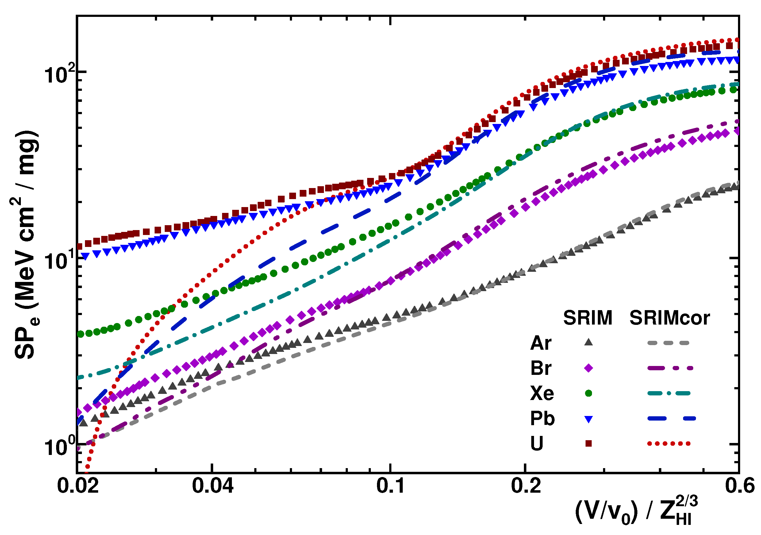
In Figure 31, some examples of the electronic stopping-power SRIM values corrected with Equation (11) are shown in comparison to the original ones [1]. As one can see, the corrections become significant for the most heavy Pb and U ions at velocities $(V/v_0)/Z_{\mathrm{HI}}^{2/3}\lesssim 0.1$. Clearly, such behavior is determined by the availability of the $S{P}_e$ data [11] at $0.8v_0$.

Figure 31. The electronic stopping-power SRIM values corrected with Equation (11) (lines) are shown in comparison to the original SRIM values [1] for Ar, Br, Xe, Pb, and U ions (small symbols) at low velocities.

Figure 31. The electronic stopping-power SRIM values corrected with Equation (11) (lines) are shown in comparison to the original SRIM values [1] for Ar, Br, Xe, Pb, and U ions (small symbols) at low velocities.

Now, with the correction functions for $S{P}_{tot}^{\mathrm{SRIM}}$ and $S{P}_e^{\mathrm{SRIM}}$, which correspond to Equation (8) and Equation (11), respectively; Equation (10) can be rewritten as

$$S{P}_n^{\mathrm{expt}}=f_{tot}^{cor}\left(V_r\right)S{P}_{tot}^{\mathrm{SRIM}}-f_{el}^{cor}\left(V_r\right)S{P}_e^{\mathrm{SRIM}},$$

(12)

and thus, the nuclear stopping power could be empirically estimated for the specified HI. The $S{P}_n^{\mathrm{expt}}$ values are determined by the parameter values of the $f_{tot}^{cor}\left(V_r\right)$ and $f_{el}^{cor}\left(V_r\right)$ functions listed in Table 1 and Table 2, respectively, and the average value a.

3.3. Nuclear Stopping Power Estimates

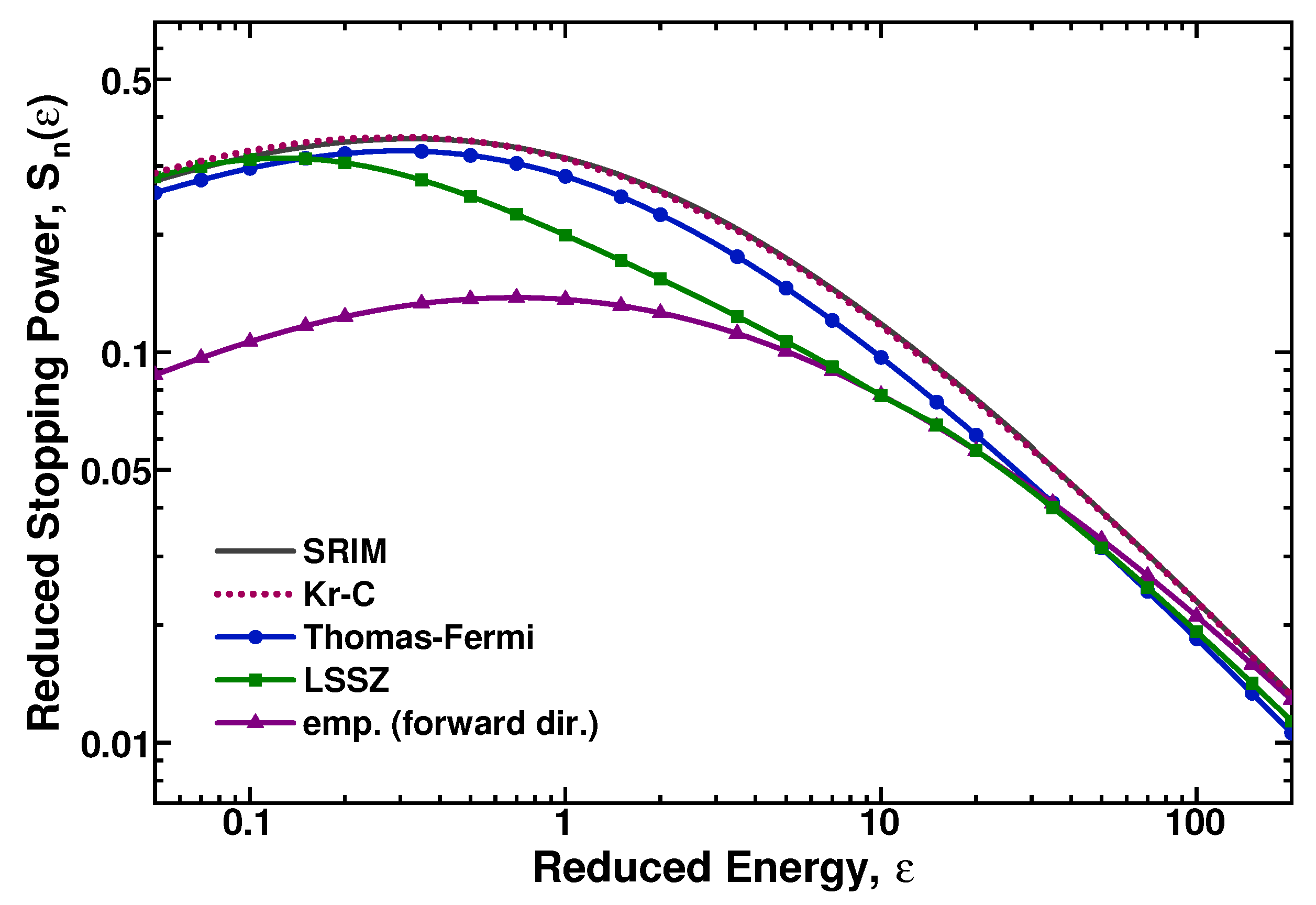
For the orientation, the different nuclear SP approximations mentioned in Section 2.2 are shown in Figure 32 in the common form of reduced $S_n\left(\epsilon \right)$ functions. These functions are compared with the “universal” nuclear stopping power used in SRIM calculations:

$$\begin{array}{ccc}\hfill S_n^{\mathrm{SRIM}}\left(\epsilon \right)& =& \hfill \frac{0.5ln(1+1.1383\epsilon )}{\epsilon +0.01321{\epsilon }^{0.21226}+0.19593{\epsilon }^{0.5}},\epsilon ⩽30;\hfill \\ \hfill S_n^{\mathrm{SRIM}}\left(\epsilon \right)& =& \hfill 0.5ln\left(\epsilon \right)/\epsilon ,\phantom{ln(1+1.13831\epsilon )/\epsilon /\epsilon }\epsilon >30;\hfill \end{array}$$

(13)

where the reduced energy is determined as

$$\epsilon =32.53A_{t}E/\left[(A_{\mathrm{HI}}+A_t)Z_{\mathrm{HI}}{Z}_t(Z_{\mathrm{HI}}^{0.23}+Z_t^{0.23})\right].$$

(14)

An empirical formula [14] is also shown in Figure 32, which corresponds to the data obtained in measurements made in a forward direction along the beam axis within a narrow acceptance angle (as mentioned in Section 1):

$$S_n^{\mathrm{emp}}=0.75\frac{ln(0.78{\epsilon }^{0.5}+1)}{{(0.78{\epsilon }^{0.5}+1)}^2},$$

(15)

where $\epsilon$ is determined by Equation (4). The approximation expressed by Equation (6) (as “the best” one considered in [19]) is also added to the figure. It uses $\epsilon$ values corresponding to a screening length

$$a_{scr}=0.8853a_0/{(Z_{\mathrm{HI}}^{1/2}+Z_t^{1/2})}^{2/3},$$

(16)

where $a_0$ is the Bohr radius, whereas $\epsilon$ values determined using Equation (4) correspond to the respective screening length definition [18]. For $S_n\left(\epsilon \right)$ determination, approximate scaling was earlier proposed [36], with the use of the integtation of scaling function $f\left(\eta \right)$. The last, in turn, is determined by the parameters of the specified interaction potential (see, for example, [18]). In the present work, $f\left(\eta \right)$, corresponding to the Thomas-Fermi potential was integrated, and the results thus obtained are also shown in Figure 32.

Figure 32. Some approximations for reduced nuclear stopping power $S_n\left(\epsilon \right)$ are shown: the one used in the SRIM calculation [1] (solid line), and those considered in this section and in Section 2.2. The last instances are designated as “emp. (forward dir.)” [14] “LSSZ” [17], “Thomas-Fermi” [18,36] (different symbols connected by solid lines), and “Kr-C” [19] (dotted line). See the text for details.

Figure 32. Some approximations for reduced nuclear stopping power $S_n\left(\epsilon \right)$ are shown: the one used in the SRIM calculation [1] (solid line), and those considered in this section and in Section 2.2. The last instances are designated as “emp. (forward dir.)” [14] “LSSZ” [17], “Thomas-Fermi” [18,36] (different symbols connected by solid lines), and “Kr-C” [19] (dotted line). See the text for details.

As one can see in the figure, all approximations give close $S_n$ values at $\epsilon \gtrsim 10$, whereas at $\epsilon \lesssim 10$, they are varied, and the difference from $S_n^{\mathrm{emp}}$ reaches a factor of ∼3 at $\epsilon =0.1$. At the same time, the low-velocity approximations considered here correspond to $\epsilon \gtrsim 2$, which may restrict the opportunity for the $S_n\left(\epsilon \right)$ extrapolation by values of $\epsilon \gtrsim 1$. Further, the $S_n\left(\epsilon \right)$ values converted from $S{P}_n^{\mathrm{expt}}$ obtained with Equation (12) are compared with the SRIM and empirical approximations [1,14] given by Equations (13) and (15), respectively.

Different behaviors of nuclear stopping, arising as a result of the application of Equation (12) application and its subsequent conversion into reduced $S_n\left(\epsilon \right)$ values, could be reproduced by three different approximations, corresponding to three groups of HIs. These seem to be quite unexpected results, which are shown in Figure 33, Figure 34 and Figure 35.

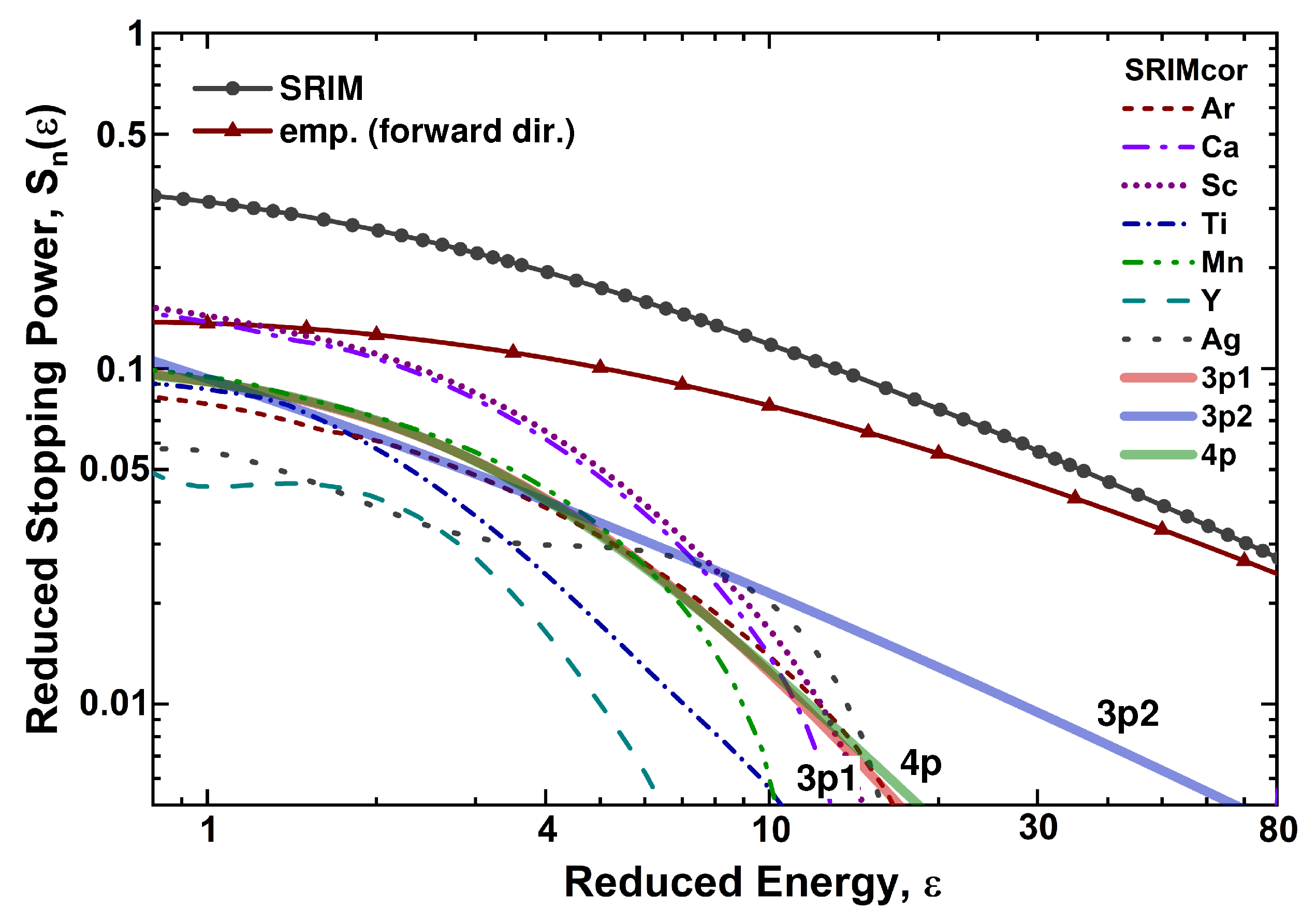
The $S_n\left(\epsilon \right)$ functions for the Ar, Ca, Sc, Ti, Mn, Y, and Ag ions are shown in Figure 33. These functions have similar behaviors, differing by a factor of ∼2. At $\epsilon \lesssim 2$, the $S_n$ values for Ar, Ca, Sc, Ti, and Y approach those given by Equation (15). At the same time, all the functions show a steep fall in the $S_n$ values at $\epsilon \gtrsim 2$, as compared with SRIM and empirical approximations [1,14]. In view of uncertainties in the $S{P}_n^{\mathrm{expt}}$ estimates, this data set and two others could be approximated by the “universal” expressions [19] fitted with their respective parameters:

$$\begin{array}{ccc}\hfill S_n& =& \hfill [0.5ln(1+A\epsilon )]/(\epsilon +B{\epsilon }^C),\hfill \end{array}$$

(17)

$$\begin{array}{ccc}\hfill S_n& =& \hfill [Aln\left(B\epsilon \right)]/[B\epsilon -1/{\left(B\epsilon \right)}^C],\hfill \end{array}$$

(18)

$$\begin{array}{ccc}\hfill S_n& =& \hfill 1/(4+A/{\epsilon }^B+C/{\epsilon }^D),\hfill \end{array}$$

(19)

where A, B, C, and D are the fitting parameters. The unweighted LSM for fitting was applied to the obtained $S_n\left(\epsilon \right)$ functions relating to the specific set of HIs. The $S_n\left(\epsilon \right)$ changes were limited by ranges of $0.8\lesssim \epsilon \lesssim 80$ and $S_n\gtrsim 0.005$. The 3p1 and 4p expressions (Equations (17) and (19), respectively) correspond to the best fits as compared to the 3p2 expression (Equation (18)), according to the ${\chi }^2$ criterion. The results of fitting are shown in Figure 33, and the parameter values obtained for the best Ar–Ag fitting are listed in Table 3.

Figure 33. The $S_n\left(\epsilon \right)$ functions obtained for Ar, Ca, Sc, Ti, Mn, Y, and Ag with Equation (12) are shown by respective intermittent lines. These are compared to SRIM and empirical approximations [1,14], expressed by Equations (13) and (15) (symbols connected by respective solid lines). $S_n\left(\epsilon \right)$ obtained with Equations (17)–(19) fittings to this HI set are shown by thick solid lines denoted as 3p1, 3p2, and 4p.

Figure 33. The $S_n\left(\epsilon \right)$ functions obtained for Ar, Ca, Sc, Ti, Mn, Y, and Ag with Equation (12) are shown by respective intermittent lines. These are compared to SRIM and empirical approximations [1,14], expressed by Equations (13) and (15) (symbols connected by respective solid lines). $S_n\left(\epsilon \right)$ obtained with Equations (17)–(19) fittings to this HI set are shown by thick solid lines denoted as 3p1, 3p2, and 4p.

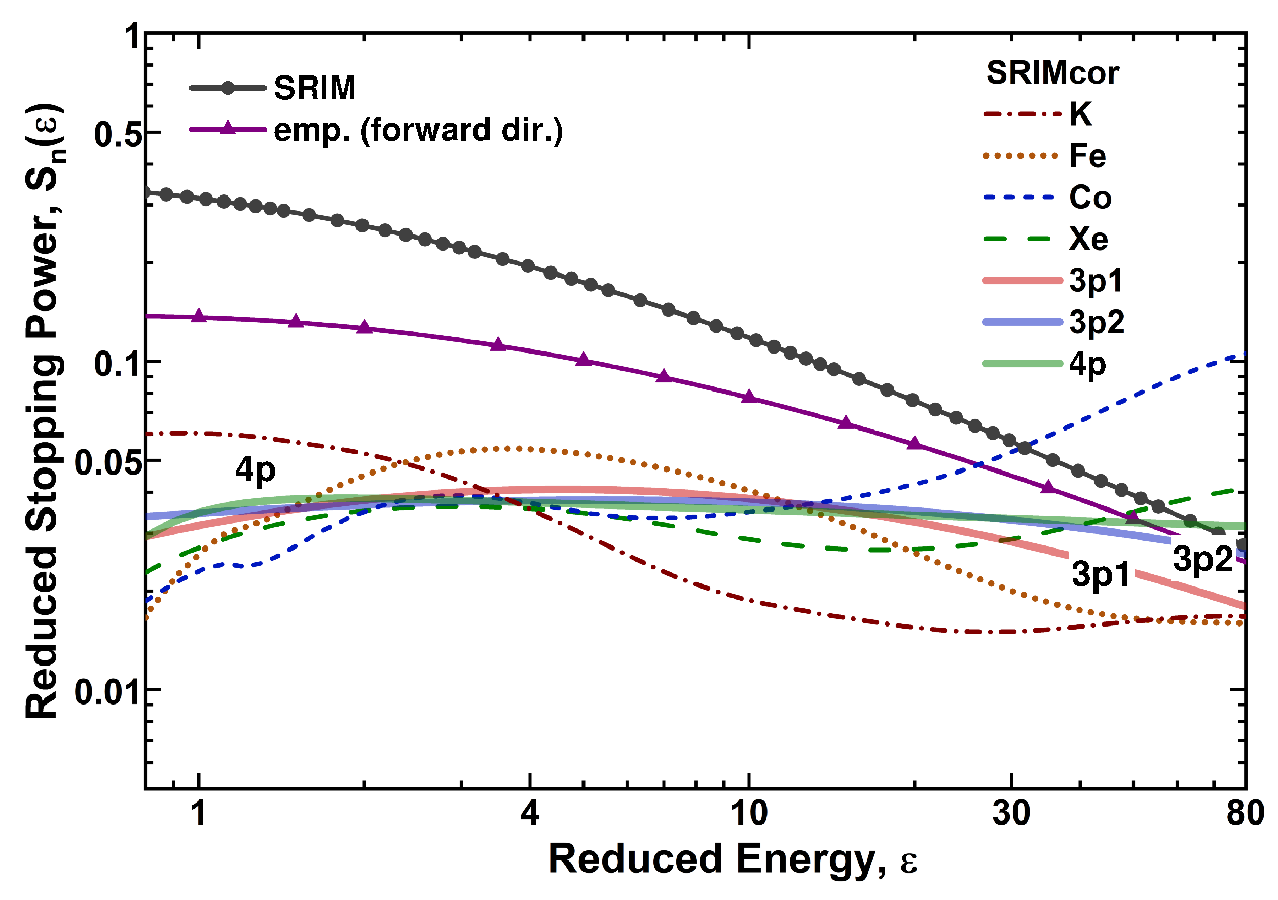
In Figure 34, the $S_n\left(\epsilon \right)$ functions for the K, Fe, Co, and Xe ions are shown. They differ from each other by a factor of ∼3 at $\epsilon \lesssim 10$ and show a larger difference in the $S_n$ values at $\epsilon \gtrsim 10$. The behaviors of the $S_n$ values for these HIs differs from that obtained for the previous HI group and from calculations according to the SRIM and empirical approximations [1,14]. The approximations with Equations (17)–(19) did not show a good fit to the $S_n$ dependencies for these HIs. The unexpected behaviors of the fitted $S_n$ dependencies implies that nuclear stopping is about the same in the energy range under consideration and plays a minor role for this HI set at low energies, as compared to the previous Ar–Ag case and to the approximations [1,14]. The best fit $S_n\left(\epsilon \right)$ thus obtained approaches the approximations [1,14] at $\epsilon \gtrsim 30$, and gives lower values than those by a factor of 4–10 at $\epsilon \lesssim 10$. The best fit is with the 3p1 expression (Equation (17)) using a fixed value of the B parameter. The parameter values corresponding to this fit are listed in Table 3.

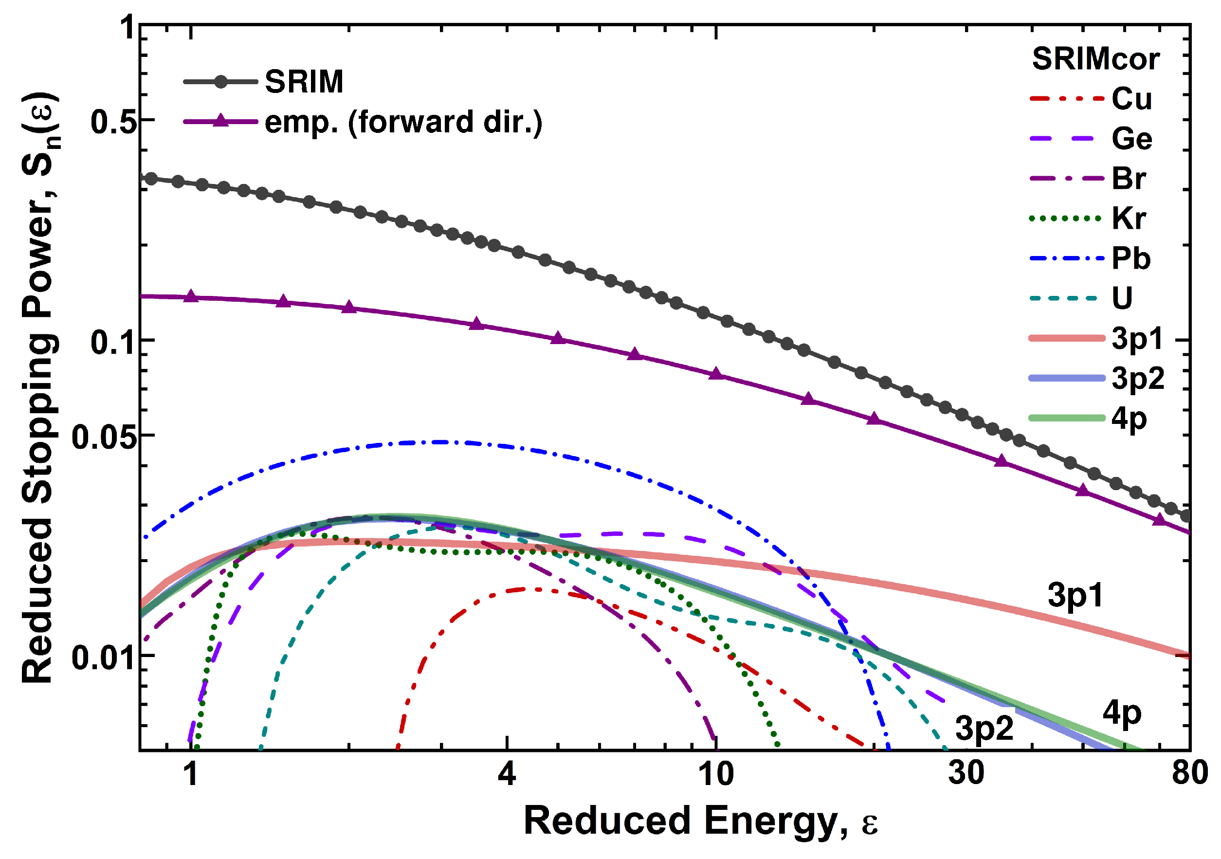
The $S_n\left(\epsilon \right)$ functions for Cu, Ge, Br, Kr, Pb, and U ions are shown in Figure 35. In contrast to the previous cases, nuclear stopping is only manifested at $\epsilon \lesssim 25$. The $S_n\left(\epsilon \right)$ approximations fitted to these functions have a maximum at $\epsilon \simeq 3$. The maximum value is lower than the values given by the SRIM and empirical approximations [1,14] by a factor of 5–7 at this energy. The $S_n\left(\epsilon \right)$ functions obtained with the 3p1 and 4p expressions (Equations (18) and (19), respectively) close to these functions. The best-fitting parameter values for this HI set are listed in Table 3.

Figure 34. The same as in Figure 33, but for K, Fe, Co, and Xe.

Figure 34. The same as in Figure 33, but for K, Fe, Co, and Xe.

Figure 35. The same as in Figure 33 and Figure 34, but for Cu, Ge, Br, Kr, Pb, and U.

Figure 35. The same as in Figure 33 and Figure 34, but for Cu, Ge, Br, Kr, Pb, and U.

Table 3. The A, B, C, and D parameter values are listed as the result of the best-fitting $S_n\left(\epsilon \right)$ functions using Equations (17)–(19) applied to each HI set. The $S_n\left(\epsilon \right)$ dependencies obtained for different HIs were combined into three sets (indicated in the first column) corresponding to the similarity in the $S_n\left(\epsilon \right)$ behavior. The results of data fitting are also shown in Figure 33, Figure 34 and Figure 35.

HI set	Equation	A	B	C	D
Ar–Ag	(17)	0.229 ± 0.023	0.127 ± 0.080	2.48 ± 0.34
K–Xe	(19)	20.89 ± 1.47	−0.065 ± 0.029	3.94 1	3.94 1
Cu–U	(18)	0.0728 ± 0.0033	1.06 ± 0.12	3.38 ± 0.89

¹ Fixed value, corresponding to the best fit.

Table 3. The A, B, C, and D parameter values are listed as the result of the best-fitting $S_n\left(\epsilon \right)$ functions using Equations (17)–(19) applied to each HI set. The $S_n\left(\epsilon \right)$ dependencies obtained for different HIs were combined into three sets (indicated in the first column) corresponding to the similarity in the $S_n\left(\epsilon \right)$ behavior. The results of data fitting are also shown in Figure 33, Figure 34 and Figure 35.

HI set	Equation	A	B	C	D
Ar–Ag	(17)	0.229 ± 0.023	0.127 ± 0.080	2.48 ± 0.34
K–Xe	(19)	20.89 ± 1.47	−0.065 ± 0.029	3.94 1	3.94 1
Cu–U	(18)	0.0728 ± 0.0033	1.06 ± 0.12	3.38 ± 0.89

¹ Fixed value, corresponding to the best fit.

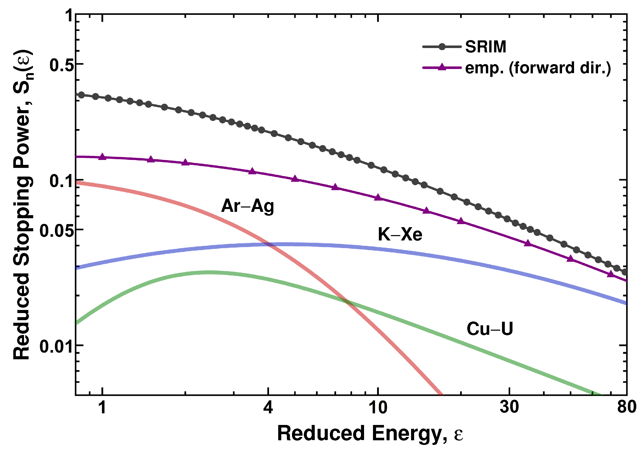
In Figure 36, the best-fit $S_n\left(\epsilon \right)$ functions obtained from the analysis of the Ar–Ag, K–Xe, and Cu–U sets, which correspond to the parameter values listed in Table 3, are shown in comparison to the approximations [1,14].

4. Discussion

A quantitative comparison of the carbon SP data obtained at $0.8v_0$ to similar ones obtained with SRIM/TRIM model calculations/simulations [1] showed the disadvantages of the latter in reproducing both the total and electronic SP values for HIs. For ions heavier than Xe, the model overestimates electronic SP by a factor reaching 2.5, as compared to the data [11], whereas for the lighter ions, the disagreements amount to within +5% to −20% of the data [9,10] and to within −10% to −30% of the data [11] (see Figure 1 and Figure 4). The ∼20% difference between the electronic SP data [9,10] and those in [11] could be explained by the difference in the detection angle in the forward direction, relative to the beam axis, for HIs escaping a target, as well as the different options for the nuclear (elastic) SP accounting in a subsequent subtraction of this value from the measured one.

In describing other results of the experiments [9,10,11], TRIM simulations showed a remarkable overestimation in the energy distribution width for Ar ions passing through a thin target (∼7 $\mathsf{\mu }$g/cm${}^2$) in comparison to the value obtained in the experiment [9] (see Figure 2). That was in contrast to a similar comparison for Xe ions passing through a thick target (∼30 $\mathsf{\mu }$g/cm${}^2$), for which the measured [11] and simulated widths have been found to be about the same (see Figure 3). Further comparison for HIs escaping the targets in a forward direction (the same conditions as in measurements) and for those escaping at all angles, showed that, according to simulations, one may expect an 8.3% and 4.6% decrease in total SP values for Ar and Xe ions, respectively, for HIs escaping the targets in a forward direction (see Figure 2 and Figure 3).

Some differences in the total SP values for Cu ions for a thin (∼5 $\mathsf{\mu }$g/cm${}^2$) and a relatively thick target (∼30 $\mathsf{\mu }$g/cm${}^2$) were also revealed in TRIM simulations as compared to the experiments [10,11] (see Figure 5). Thus, these overestimates in the simulations for the thin target corresponded to 6.5% and 48%, as compared to the experimental data [10] and [11], respectively. Simulations also showed the independence of the SP of the output angle in a forward direction for HIs escaping the target, at least at $0.{15}^{\circ }\lesssim {\theta }_{\mathrm{out}}\lesssim 1.5^{\circ }$. For the relatively thick target, however, TRIM overestimated the measurements [11] by 28%.

The results of the analysis, as a whole, allowed us to state that SRIM/TRIM calculations/simulations remarkably overestimate carbon total stopping powers [11] at a HI velocity of $0.8v_0$. At the same time, the electronic SP data [9,10] for C to Y ions are in satisfactory agreement with the calculations/simulations.

The SP data [9,10,11] considered within the LSS approach [15] as an alternative to SRIM/TRIM calculations/simulations are not reproduced using different approximations for nuclear stopping. Although the electronic SP data could be described as “on average,” the $Z_{\mathrm{HI}}$ oscillations observed in the experiments [9,10,11] are not reproduced in the LSS calculations [15]. The addition of the calculated nuclear SPs [17] leads to an excess of calculations over the experimental total SP data, which implies overestimates of the nuclear SP values (see Figure 6 and Figure 7).

Further analysis of the total and electronic SP data revealed that the reduced nuclear stopping powers $S_n\left(\epsilon \right)$ for HIs from Ar to U at $0.8⩽\epsilon ⩽80$ were generally lower than those predicted by any approximation [1,14,15,17,19,36]. This reduction depends on the reduced energy (velocity) of HI, and unexpectedly, on the HI atomic number. The last dependence appeared in the similarity of $S_n\left(\epsilon \right)$ variations for the specified HIs, which enabled their grouping into definite sets and fitting by different functions, as shown in Figure 36.

In search of the causes of such nuclear SP behavior, it should be noted that nuclear stopping is determined by interatomic potential $U\left(r\right)$ describing the interaction of HI and atoms of the medium. These potentials were determined for 14 atomic systems using approximations to the results obtained with the free-electron method [19]. Thus, the obtained approximations were expressed as

$$U(r/a_{scr})=(Z_{\mathrm{HI}}{Z}_t{e}^2/r)\sum _{i=1}^3{C}_{i}exp(-b_{i}r/a_{scr}),$$

(20)

where r is the interatomic separation, e is the electronic charge, $C_i$ and $b_i$ are fitting constants, and $a_{scr}$ is a screening radius (length) according to Equation (16).

In TRIM simulations, interatomic interactions are determined via the Ziegler-Biersack-Littmark (ZBL) Universal Screening Potential [19,38]. The ZBL potential is similar to Equation (20), but it uses eight fitting parameters ($i=4$) and is based on the calculated solid-state interatomic potentials of 522 randomly chosen pairs of atoms in the range of 1–82 for $Z_{\mathrm{HI}}$ and $Z_t$, as described in [38]. A screening length is defined as

$$a_{scr}=0.8854a_0/(Z_{\mathrm{HI}}^{0.23}+Z_t^{0.23}).$$

(21)

One can speculate about reproducing the $S_n\left(\epsilon \right)$ variations obtained here in calculations using the interatomic potential(s) according to Equation (20). Thus, one may mean specific values of the $C_i$, $b_i$, and $a_{scr}$ parameters that correspond to a specific potential for the pair of colliding atoms. In this regard, the energy dependence of the ion charge inside the matter will determine the $a_{scr}\left(\epsilon \right)$ dependence. On the other hand, the interatomic potentials similar to Equation (20) do not take into account the atomic shell structures of ions moving inside the matter. This structure may affect ion charge states, making them different from those determined using $a_{scr}$ and thereby affecting collisional SP values.

5. Conclusions

Quantitative estimates of the nuclear (collisional) stopping power component of carbon for heavy ions were considered using the available data for 16 low-energy projectiles from Ar to U. The nuclear (collisional) carbon stopping power was found to be significantly lower than those predicted by any of the “universal” approximations [1,14,15,17,19,36], at least for the case under consideration. This reduction depended on reduced energy $\epsilon$ ($0.8\lesssim \epsilon \lesssim 80$), and quite unexpectedly, on the ion atomic number $Z_{\mathrm{HI}}$. The considered data correspond to 21% of all projectiles, for which the stopping powers could be studied.

The lack of stopping power data for most heavy atoms ($Z_{\mathrm{HI}}>54$) could be filled using a consideration of their ranges obtained at lower energies [39], as well as the ranges of evaporation residues (ERs) produced in nuclear fusion–evaporation reactions induced by heavy ions [40]. In these studies, a remarkable excess of the ranges for stable atoms of Eu, Er, Yb, and Pb, as well as for Tb, Dy, Po, At, Rn, and Ac ERs stopped in C and Al, respectively, over those predicted using SRIM/TRIM calculations/simulations [1] was observed. Artificial low-energy radioactive atoms are inaccessible as projectiles used in stopping power experiments, whereas they can be produced in sufficient amounts in the nuclear reactions, allowing for an extension of studies for most heavy atoms.

In continuation of this study, it is of interest to analyze the low-energy stopping power data for lighter and heavier media. Such an analysis may help to derive an empirical universal scaling for the low-energy nuclear stopping power for ions and media of any atomic number as a function of the (reduced) energy. In the case of the universality of the nuclear-stopping reducing phenomenon, theoretical models describing this phenomenon will be of interest either in its understanding or its practical usage.