Article

Deep Learning of Quasar Lightcurves in the LSST Era

by
Andjelka B. Kovačević
1,2,*,
Dragana Ilić
1,3,
Luka Č. Popović
1,2,4,
Nikola Andrić Mitrović
5,
Mladen Nikolić
1,
Marina S. Pavlović
6,
Iva Čvorović-Hajdinjak
1,
Miljan Knežević
1 and
Djordje V. Savić
4,7
1
Faculty of Mathematics, University of Belgrade, Studentski trg 16, 11000 Belgrade, Serbia
2
PIFI Research Fellow, Key Laboratory for Particle Astrophysics, Institute of High Energy Physics, Chinese Academy of Sciences, 19B Yuquan Road, Beijing 100049, China
3
Humboldt Research Fellow, Hamburger Sternwarte, Universitat Hamburg, Gojenbergsweg 112, 21029 Hamburg, Germany
4
Astronomical Observatory, Volgina 7, 11000 Belgrade, Serbia
5
Department of Mathematics “Tullio Levi Civita”, University of Padova, Via Trieste, 35121 Padova, Italy
6
Mathematical Institute of the Serbian Academy of Sciences and Arts, Kneza Mihaila 36, 11000 Belgrade, Serbia
7
Institut d’Astrophysique et de Géophysique, Université de Liège, Allée du 6 Août 19c, 4000 Liège, Belgium
*
Author to whom correspondence should be addressed.
Universe 2023, 9(6), 287; https://doi.org/10.3390/universe9060287
Submission received: 10 February 2023 / Revised: 2 June 2023 / Accepted: 9 June 2023 / Published: 11 June 2023

Abstract

:
Deep learning techniques are required for the analysis of synoptic (multi-band and multi-epoch) light curves in massive data of quasars, as expected from the Vera C. Rubin Observatory Legacy Survey of Space and Time (LSST). In this follow-up study, we introduce an upgraded version of a conditional neural process (CNP) embedded in a multi-step approach for the analysis of large data of quasars in the LSST Active Galactic Nuclei Scientific Collaboration data challenge database. We present a case study of a stratified set of u-band light curves for 283 quasars with very low variability ∼0.03. In this sample, the CNP average mean square error is found to be ∼5% (∼0.5 mag). Interestingly, besides similar levels of variability, there are indications that individual light curves show flare-like features. According to the preliminary structure–function analysis, these occurrences may be associated with microlensing events with larger time scales of 5–10 years.

1. Introduction

The launch of the Legacy Survey of Space and Time (LSST), which will be conducted by the Vera C. Rubin Observatory, is currently scheduled to take place in the first half of 2024. The cadences of the LSST, in concert with its large observational coverage, will capture a wide variety of intriguing time domain events, some of which are periodic signals of interest [1]. LSST should probe time series with cadences ranging from one minute to ten years across not only a vast portion of the sky but also across five photometric bands (see Figure 1).
Such synoptic (multi-band and multi-epoch) cadences combined with the large coverage will enable us to detect very short-lived events such as eclipses in ultracompact double-degenerate binary systems [2], fast faint transients such as optical phenomena associated with gamma-ray bursts [3], and  electromagnetic counterparts to gravitational wave sources [4,5]. In contrast, the LSST decadal data catalogs will make it possible to investigate long-period variables, intermediate-mass black holes (IMBH), and quasars (QSO) [6,7,8,9,10].
Figure 1. Schematic view of the LSST third scientific pillar. Exploring the transient optical sky as defined in Ivezić et al. [1]. The broad range of probed time scales and sky area may allow for the search for general variability properties across different types of objects, similar to the study by Burke et al. [10], which suggests a common process for all accretion disks. The references Anderson et al. [2], Bloom et al. [3], Scolnic et al. [4], Kaspi et al. [6], MacLeod et al. [7], Graham et al. [8], Chapline and Frampton [9] given in boxes are further explained in the text.
Universe 09 00287 g001
Quasars are an important population to study in order to have a better grasp of the physics behind the accretion of matter when it is subjected to extremely harsh conditions. Moreover, studies show that they may be used as cosmological probes (e.g., [11,12]). Up to this point, several hundred thousand quasars have been spectroscopically confirmed, and numerous efforts have been undertaken to identify the properties of their temporal flux variability [13]. The proposed physical mechanisms underlying the optical/UV variability range from the superposition of supernovae (e.g., [14]), microlensing [15,16], and thermal fluctuations from magnetic field turbulence [17] to instabilities in the accretion disk [14]. The amplitude of quasar observed optical variability is typically a few tenths of a magnitude (e.g., [18] found the SDSS quasars variability is ∼0.03 mag with a characteristic time-scale of several months) but it can also show larger variations over longer time-scales (see [19,20]), with statistical description via a damped random walk (DRW) model (e.g., [17,20,21]). The long lasting flare-like events (extreme tails of the variability distribution) are less clearly defined and represent a distinct kind of modeling problem (see, e.g., [22] and references therein). On top of this, the light curves have different topologies, which are superimposed on different types of cadences, which imposes many difficulties onto their modeling and the process of extracting knowledge from them 1.
Specifically, the LSST will provide a breakthrough in quasar observations in survey area and depth [23] as well as variability information of light curves sampled at a relatively high cadence (the order of days), over the course of a decade of the operations. Because of these new qualities, the LSST will be able to search even for supermassive black hole (SMBH) binaries having shorter periods (<5 years), which are significantly more uncommon. For instance, Xin and Haiman [23] suggested that it might be possible to identify ultra-short-period SMBH binaries (periods < 3 days) in the LSST quasar catalog. These binaries are thought to be so compact that they will ’chirp’, or evolve in frequency, into the gravitational wave band, where the Laser Interferometer Space Antenna (LISA [24]) will be able to detect them in the middle of the 2030s. The expectations of such exciting discoveries are probable [23], as massive binary SMBHs are predicted to spend O ( 10 5 ) years in orbits with periods of the order of a year if orbital decay is caused by either gravitational wave emission or negative torques exerted on the viscous time-scale by the surrounding gas disc [25].
Even while the LSST have cadences that are unprecedented in contrast to those of its predecessors, these cadences will primarily take the shape of more or less regular samplings that are separated by various short or lengthy periods (seasons) in which there are no observations.
When attempting to evaluate the variable features of quasar light curves, these frequent gaps represent one of the most challenging obstacles to overcome (along with the obviously irregular cadences, see [21]). In quasar time domain analysis, there are two main ways to deal with sampling that is not even in stochastic light curves [21]: the first approach is to use Monte Carlo simulations to forward the model in the frequency domain (see, e.g., [26]), whereas the second approach is to fit the light curve in the time domain mostly using Gaussian Processes (GP, see [27]).
Both approaches are viable, although they can be computationally expensive (see details in [21] and the references therein). If the cadences are similar to those found in the LSST with seasonal gaps, the first method is a costly one to compute because it necessitates either creating a highly dense light curve at the optimal sampling rate or segmenting the light curve and computing the periodograms of each segment separately. The likelihood function of GP, on the other hand, is computationally expensive (scales O ( n 3 ) ) for the second approach because it requires inverting the n × n covariance matrix of the light curve, where n is the number of data points. A first-order continuous-time autoregressive process (CAR(1)) or an Ornstein–Uhlenbeck process, which could represent quasar light curves, is a special class of GP for which the computational complexity only scales linearly with the length of the light curve [17]. The application of CAR(1) to modeling typical active galactic nuclei (AGNs) optical light curves is questioned (see [20]), as some studies have found evidence for deviations from the CAR(1) process for optical light curves of AGN (see, e.g., [8,28,29]). Due to the nature of this issue, it was necessary to develop more complex Gaussian random process models, such as the continuous auto-regressive moving-average models (CARMA, [21]). Moreover, it has been demonstrated by Yu et al. [30] that a second-order stochastic process, a damped harmonic oscillator (DHO), is a more accurate way to characterize the variability of AGNs. Based on previous examples, the evolution of algorithms used to model AGN light curves typically emphasizes an increase in the total number of needed parameters. All of these models, however, are based on information gathered before the LSST era, which has a tendency to favor more luminous and nearby AGNs. Therefore, in order to make use of the tens of millions of the LSST AGN multi-band light curves effectively, it is highly desirable to employ flexible data-driven machine learning algorithms.
At the moment, kernel methods (such as GPs) and deep neural networks are seen as two of the most remarkable machine learning techniques [31]. The relationship between these two approaches has been the subject of a great deal of research in recent years [31,32]. In this light, here we present the AGN light curve modeling unit, which was created as a preprocessing module of the SER-SAG 2 team’s LSST in-kind contribution of the time-domain periodicity mining pipeline and combines the best of two machine learning worlds. The neural latent variable model [Neural Process-NP [33]] is at the heart of this modeling unit. NPs, such as GPs, create distributions over functions, can adapt quickly to new observations, and can assess the uncertainty in their predictions [33]. NPs, such as neural networks, are computationally efficient during training and assessment, but they also learn to adapt their priors to data as well [33]. The NP module has been trained on the quasar light curves found in a dedicated database that arose from a challenge focused on the future use of the LSST quasar data (LSST_AGN_DC [34]). During the course of the operation, we also came to the realization that it is possible to distinguish the variable properties of quasars.
In our previous work (see [35] hereafter Paper I), we adapted a conditional neural process (CNP) for modeling the general variability of quasar light curves on a smaller sample of tens of objects. In this work, we complement the study of Paper I with an upgraded version of CNP on a much larger database of (∼4 × 10 5 ) quasars (LSST_AGN_DC) which demanded ’deep learning’ through a multi-step process and provide a case study example of how a complex procedure of ’deep learning’ of quasar variability may lead to surprising results, i.e., detection of a larger collection of quasars with flare-like events. These flare-like incidents occur over a longer time period, and the preliminary structure–function analysis suggests that they may be related to microlensing events.
It is anticipated that the LSST would lead to an increase of at least one order of magnitude in the number of lensed quasars that are known [36]. Thus, optimizing the analysis or selecting sub-samples of those systems is becoming important (e.g., [37]).
The structure of the paper is as follows. In Section 2, we describe the data used for the machine learning experiments. In Section 3, we provide a concise explanation of the machine learning methods that were applied; while in Section 4, we report and discuss in further detail the series of experiments that were carried out. In the final Section 5, we summarize our findings.

2. Materials

2.1. Description of Quasar Data in LSST_AGN_DC

The dataset of AGN light curves used for the demonstration of our neural process modeling unit is selected from the LSST AGN data challenge 2021 dataset [LSST_AGN_DC, see details in [34]). The LSST_AGN_DC mimics the future LSST data release catalogs as much as possible (see also [38]). Calculations were run on NVIDIA T4, 2560 CUDA cores, Compute capability 7.5, Memory 16 GB GDDR6, Max memory bandwidth 300 GB/s.
The total number of objects in the LSST_AGN_DC is ∼440,000, with stars, galaxies, and 39,173 quasars drawn from two main survey fields, an expanded Stripe 82 area, and the XMM-LSS region. The total number of epochs for all objects is ∼5 ×   10 6 [34]. The quantity of features (parameters) of objects is 381, sorted as (see details in [34,38]) astrometry (celestial equatorial coordinates, proper motion, parallax); photometry (point and extended source photometry in AB magnitudes and fluxes (in nano-Jansky); color (derived from flux ratio between different photometric bands); morphology (continuous number in range [ 0 ,   1 ] , extended sources has morphology closer to 1, while point-like sources closer to 0); light curve features (extracted from SDSS); spectroscopic and photometric redshift; and class labels (Star/Galaxy/quasar). The time domain data of light curves include observation epochs, photometric magnitudes, and errors in u,g,r,i,z bands as well as periodic and non-periodic features (see description of features in [39]).

2.2. Sample Selection

We chose 1006 quasars, that are spectroscopically confirmed and which have ≥100 epochs in u-band light curves (see Figure 2) from this large initial database. We employ this criterion because earlier research has demonstrated that this number of points is acceptable for both modeling light curves and extracting periodicity (see, e.g., [40]). We selected to study u-band light curves since they are less deformed by photometric filters [41]. In terms of mean sampling, the chosen quasar subsample exhibits a stratification into three non-intersecting branches of mean sampling (Figure 2).
Both the non-Gaussianity of marginal distributions and stratification in the phase space of mean sampling and the number of points in the light curves indicate that we are encountering a highly diverse sample.
Kasliwal et al. [42] provided the first case study of the relevance of using modeling procedures individually on stratified light curves, as opposed to the “one-size-fits-all” approach, which allows us to account for the prevailing physical process’s heterogeneity. The authors categorized the Kepler light curves of 20 objects based on visual similarities and found that the light curves fall into five broad strata: stochastic-looking, somewhat stochastic-looking+weak oscillatory features, oscillatory features dominant, flare features dominant, and not-variable. Certain light curves appear to change from one state of variability to another.
Motivated by Kasliwal et al. [42]’s example and a large number of our preselected objects (1006) that cannot be visually stratified, we employed the Self-Organizing Maps (SOM) algorithm [43] to stratify (cluster) light curves with similar topological patterns. From 36 clusters obtained from SOM, we chose interesting strata containing 310 light curves with apparent low variability (see Figure 3).
To thoroughly check the characteristics of 283 sources, we calculated the fractional root mean square (rms) variability amplitude F v a r and the optical luminosities ( L o p ).
The uncertainties of the individual magnitude measurements contribute an additional variance, which is captured in F v a r (see [44,45]) as:
S 2 = 1 N 1 i = 1 N ( m a g i < m a g > ) 2
F v a r = S 2 < σ > 2 < m a g > 2
where N is the number of points in the light curves, m a g i , i = 1 , , N are observed magnitudes, < m a g > = 1 N i = 1 N m a g i , < σ > 2 = 1 N i = 1 N σ i 2 and σ i , i = 1 , , N are measurement errors 3.
The black hole masses (M) were randomly assigned using the probability distribution based on absolute magnitude M u by [7]:
P ( log 10 M | M u ) = 1 2 π σ M 2 e x p ( log 10 M log 10 < M > ) 2 2 σ M
where log 10 < M > = 2.0 0.27 M u , σ M = 0.58 + 0.011 M u , and  M u is an absolute magnitude and is calculated using the known u-band magnitude and K-correction, K ( z ) = 2.5 ( 1 + δ ) log ( 1 + z ) , with the canonical spectral index δ = 0.5 as in Solomon and Stojkovic [46]. The assigned masses of black holes serve as proxies that complement other inferred quasar properties.
We approximate the optical luminosity ( L o p ) of the sampled objects via (see [13])
L o p [ erg s 1 ] = 4 π d L 2 F 0 , λ λ e f f 10 2.5 ( < m a g > A )
where d L is the estimated luminosity distance for a flat universe (using astropy module, [47]) with standard cosmological parameters H 0 = 67.4 km s 1 Mpc 1 and Ω m = 0.315 [48], c is the light speed, z is the redshift of the object, F 0 , λ = 3.75079 × 10 9 erg , cm 2 s 1 Å 1 is the zero point flux density, λ e f f = 3608.04 Å is the effective wavelength of the SDSS filter system (see [49,50]), < m a g > is a mean u-band magnitude, and A is the Galactic absorption at the effective wavelength along the line of sight. However, for our purposes we did not take into account A.
We present a corner plot of the four parameter distributions ( M , F v a r , L o p , z ) in Figure 4. The selected objects are indeed characterized by small variability F v a r [ 0 , 0.03 ] and larger redshift 1 z 3 . Moreover, the two-dimensional plots reveal some scatter in the parameter distributions. In contrast, the 2D distribution of luminosity and redshift of objects is strongly nonlinear, as expected (see also [13]). Finally, after excluding objects with an exact number of 100 points in the light curves, our sample contained 283 light curves with > 100 data points that were used for NP modeling.

3. Methods

In this section, we provide the motivation and description of the computational model.

3.1. Motivation

The stochastic variability seen in quasar flux time series is thought to be caused by emissions from an accretion disc with local ’spots’ that contribute more or less flux than the disc’s mean flux level. These spots appear at random and dissipate over a specific physical time scale [51]. Because the spots do not dissipate instantly within the disc, some long-term correlations may exist, which can be described by power spectrum density (PSD f 2 , where f is frequency) consistent with the Autoregressive (1) model (AR(1)), or damped random walk, or simplest form of Gaussian process characterized by the relaxation time, and the variability on timescales much shorter than relaxation time (see [17]). Some ground-based studies [8,52] show that AGN light curves could have PSD slopes steeper than AR(1) PSD on very short time scales, indicating that the damped random walk process oversimplifies optical quasar variability (see [8,53]). Moreover, Kasliwal et al. [42] developed the damped power-law (DPL) model by generalizing the PSD of AR(1) as 1 / f γ . If  γ < 2 , the process exhibits weaker autocorrelation on short time scales than the AR(1), resulting in a less smooth time series. When γ > 2 , the process exhibits stronger autocorrelation on short time scales than the AR(1), resulting in a smoother time series. However, the light curves show a wide variety of different types of behavior, even superposition of at least two features (e.g., stochastic+flare [42]). Ruan et al. [54] modeled blazar variability flare-like features with an AR(1) process using observed 101 blazar light curves from the Lincoln Near-Earth Asteroid Research (LINEAR) near-Earth asteroid survey. Moreover, Kasliwal et al. [42] tried to model flare-like features in Kepler light curves with DPL and AR(1) and point out that both models are unable to model flare-like features. Besides the variety of the strength of correlation in the AGN light curves, and different topologies of light curves, the next issue that should be taken into account is the cadence gaps (long time ranges without observation) of variable size. As we want to predict data in these gaps, it is important that we do not introduce any additional relation that could be reflected in PSD (see [29]). Various types of neural processes can be considered, such as attentive processes that can introduce attentive mechanisms for correlation among data points. However, due to large cadence gaps in quasar light curves, in Paper I, we presented the successful application of the conditional neural process (CNP, general Neural process which does not introduce correlation), combining the neural network and general Gaussian process’s capabilities, to model tens of stochastic light curves with large gaps and without flares. Here, we show an upgraded version of the code, which is applied on the quasar light curves obtained from the largest database mimicking LSST survey (LSST_AGN_DC, containing about 40,000 quasars).

3.2. Conditional Neural Process

Here, we briefly summarize the conditional neural process description; for a detailed mathematical description, the reader is referred to the given literature. It is commonly accepted in the field of machine learning that models must be “trained” with a large number of examples before they can make meaningful predictions about data they have never seen before. However, there are several instances where we do not have enough data to meet this demand: acquiring a substantial volume of data may prove prohibitively expensive, if not impossible. For example, it is not possible to obtain homogeneous cadences of observations with any ground-based telescope, including the LSST. Nonetheless, there are compelling grounds to believe that this is not a side effect of learning. Humans are known to be particularly good at generalizing after only seeing a small number of examples, according to what we know (“few-shot estimate”). In current meta-learning terminology, NPs and GPs are examples of approaches for “few-shot function estimates” [33]. NPs, as opposed to GPs, are metalearners 4 (see [55]).
We assume the latent continuous-time light curve ( x , y ) L = ( x l , y l ) l = 1 L with time instances x and fluxes y , is a realization of a stochastic process, so that observed points are sampled from it at irregular instances ( x , y ) O = ( x o , y o ) o = 1 O ) (see [56]), and which can be learned through neural processes, as it is a way to meta-learn a map from datasets to predictive stochastic processes using neural networks [55].
If we are given target inputs of time instances ( x T = x t t = 1 T ) , and corresponding unknown fluxes y T = y t T t = 1 , we need a distribution over predictions ( p ( y T | x T ; C ) )  5, where C = ( x C , y C ) = ( x c , y c ) , c = 1 , C , are context points from the light curve (used for training the model). The p ( y T | x T ; C ) distribution is called the stochastic process.
If we chose predictors at random from this distribution, each one would be a plausible way to fit the data, and the distribution of the samples would show how uncertain our predictions are. Therefore, the NP can be seen as using neural networks to meta-learn a map from datasets to predictive stochastic processes.
Generally, NPs are constructed to firstly map the entire context set to a representation R, E n c θ : C R  6, using an encoder Enc θ ( C ) = ρ c = 1 C ϕ ( x ( c ) , y ( c ) ) , where ρ , ϕ are defined by neural network [55]. The sum operation in the encoder is a key as it ensures that the resulting R “resides” in the same space regardless of the number of context points C . The predictive distribution at any set of target inputs x T is factorized and conditioned on lower dimensional representation R. Keeping this in mind, one can write that p θ ( y T | x T ; C ) = t = 1 T p θ ( y ( t ) | x ( t ) , R ) . In the next step, NP calls the decoder, Dec θ , which is the map parametrizing the predictive distribution using the target input x ( t ) and the encoding of the context set ( R ) . Typically the predictive distribution is multivariate Gaussian, meaning that the decoder predicts a mean μ ( t ) model and a variance ( σ 2 ( t ) ) [55].
Specifically, the scheme of the particular member of NP called the conditional neural process (CNP [33]) is given in Figure 5. Each pair in the context set is locally encoded by a multilayer perceptron:
R c = Enc θ ( C ) = MLP [ x ( c ) ; y ( c ) ]
Here, we discuss the main difference between the CNP and other NP: the local encodings R c are then aggregated by a mean pooling to a global representation R:
R = Enc θ ( C ) = 1 C c = 1 C MLP [ x ( c ) ; y ( c ) ]
Finally, the global representation R is fed along with the target input x t into a decoder MLP to yield the mean and variance of the predictive distribution of the target output:
( μ ( t ) , σ 2 ( t ) ) = Dec θ ( R , x ( t ) ) = MLP [ R , x ( t ) ]
The encoder consists of 1 hidden layer (dimension 2 × 128 ) that encodes the features of time instances, followed by 3 hidden layers (dimension 128 × 128 that locally encode each feature-value pair (time instances, magnitudes) with final activation ReLU layer. The decoder has a 4-hidden-layer MLP of the dimension ( 128 × 128 ) that predicts the distribution of the target value, with the last layer consisting of softmax activation function. We note that the number of layers, batch sizes, learning rates, and optimizers are chosen as a balance between the hyperparameters found in the literature where the multilayer approach is more feasible (see [13]) for our experimentation. The aim of the training CNP is to minimize the negative conditional log probability (or loss) (a more detailed explanation is given in [33,35]):
L = 1 N y T T log ( p ( y T | x T ; C ) )
where p ( y T | x T ; C ) defines a posterior distribution for target values 7 over functions that could be fitted through observed data points, and N is a cardinality of a randomly chosen subset of observations used for conditioning. An increase in the log-probability indicates that the predicted distribution better describes the data sample statistically 8.
The computational cost of prediction estimates for T target points conditioned on C context points with is O ( T + C ) , which is more efficient than for GP [33,55].
Our initial adaptation of the CNP for the purposes of the LSST quasars light curve modeling was described in Čvorović-Hajdinjak et al. [35], Breivik et al. [57]. Using the above concept, we fully developed an NP-module for LSST quasar light curve modeling, which is upgraded to pytorch and refactorized into 6 subunits:
  • Model architecture;
  • Definition of dataset class and collate function;
  • Metrics (loss and mean squared error—MSE);
  • Training and calculation of training and validation metrics (loss and MSE);
  • Saving model in predefined repository;
  • Upload of the trained model so that prediction can be performed anytime.
The following features (from the above list) are new in contrast to the earlier version of the CNP module (see [35]): (2), the MSE given in (3), as well as (5), and (6).

4. Results and Discussion

In this section, we present and discuss the results of our procedures for ’gaining the knowledge from large data’ comprising the training of CNP on strata (Section 4.1), CNP modeling of variability of light curves in strata (Section 4.2) and modified structure–function analysis of the observed and modeled light curves (Section 4.3).

4.1. Training of CNP

Following the prescription for splitting the data set into training, testing, and validating subsamples (see, e.g., [13]), we randomly divided the strata of u-band light curves (seen in Figure 5), into a training dataset with 80% of the total number of objects, a test dataset with 10% of the total number of objects, and a validation dataset with 10% of the total number of objects. The training, target, and validation time instances, originally given as modified Julian dates (MJDs), are transformed to a [ 2 , 2 ] range alongside corresponding magnitudes and measured errors 9. The training, validating, and targeting light curves are given as tensors of size 128 × N , where 128 is a batch size and N is the corresponding number of epochs in the light curves 10. We independently carried out the method of dividing the data and applying our algorithm to the training, validating, and testing data about 100 times.
During the training process, the training set was augmented by the addition of extra curves that were generated from the original by adding and subtracting measured uncertainty from observed points. The method of adding noise to neural network inputs during training has been known for a long time. Many theoretical studies have demonstrated that it allowed for increasing generalization capabilities of the network (e.g., [59,60]). Bishop [61] has shown that the use of this method was equivalent to Tikhonov regularization. Wang and Principe [62] showed that if this method was applied, the network also trained faster. Most often it is considered as one of the methods to avoid ANN overtraining (see [63]). Currently, this method is also used when training deep neural networks [64]. Noise can be introduced into a training neural network in four different phases: input data, model parameters, loss function, and sample labels (see [65,66]). For injecting the noise, it is necessary that the probability distribution from which noise is drawn corresponds to the real-world situation of observed data (see for application in astronomical light curves [67]). As photometric errors in observed light curves mostly follow Gaussian distribution (see, e.g., [19]), the added Gaussian noise ( N ( 0 , σ i ) ) to the input training light curves magnitudes corresponds to estimated measurement error( σ i ) at each time step (see for application in astronomical light curves [67]). The performance metric values for the training dataset and the validation data set for 100 runs are shown in Figure 6. The lower training loss but higher training MSE compared to the validation loss and MSE can be attributed to the sensitivity of MSE to particularly the sharp peaks in the light curves. Switching to mean absolute error (MAE) led to a more typical behavior, with the training MAE lower than the validation MAE.
As already mentioned, as a balance between hyperparameters was found in the literature and our experimentation, we used the Adam optimization algorithm (see [35] and references therein) implemented in Python package torch.optim with a learning rate of 0.0001 (see [13,67]) and a batch size of 32. Adam is probably the most frequently used optimization algorithm for training deep learning models thanks to its adaptive step size, which in practice most often leads to decreased oscillations of the gradients and faster convergence. It combines the best aspects of the AdaGrad and RMSProp algorithms to provide an optimization that can handle sparse gradients on noisy problems as we encounter in quasar light curves (see [13,67]). Once again, we emphasize that the general model was introduced in Paper I, and here we provide its upgraded version, with application on quasar light curves strata (see [68]), such granular application can potentially help the understanding of physical properties of categories of objects (see [68]), as we also demonstrated here. Moreover, CNP is well generalizable on various data sets (strata) as it inherits GP’s ability to determine the predictive distribution of data.
The left panel in Figure 6 shows that both the validation and train loss decrease rapidly until epoch 2000, after which both losses stabilize. The loss and MSE are expected to be high in the early epochs (since the network is initialized at random and the network’s behavior differs from the desired one in the early epochs) and thus inconsequential. The larger extent of epochs is depicted for illustration purposes that justify the inclusion of early stopping criterion so that CNP is trained at epochs < 2000 .
Overfitting might be indicated by a decreasing training loss and an increasing or plateauing validation loss. However, our loss curves do not show this behavior. To prevent underfitting, we employed data augmentation with noise, and early stopping.

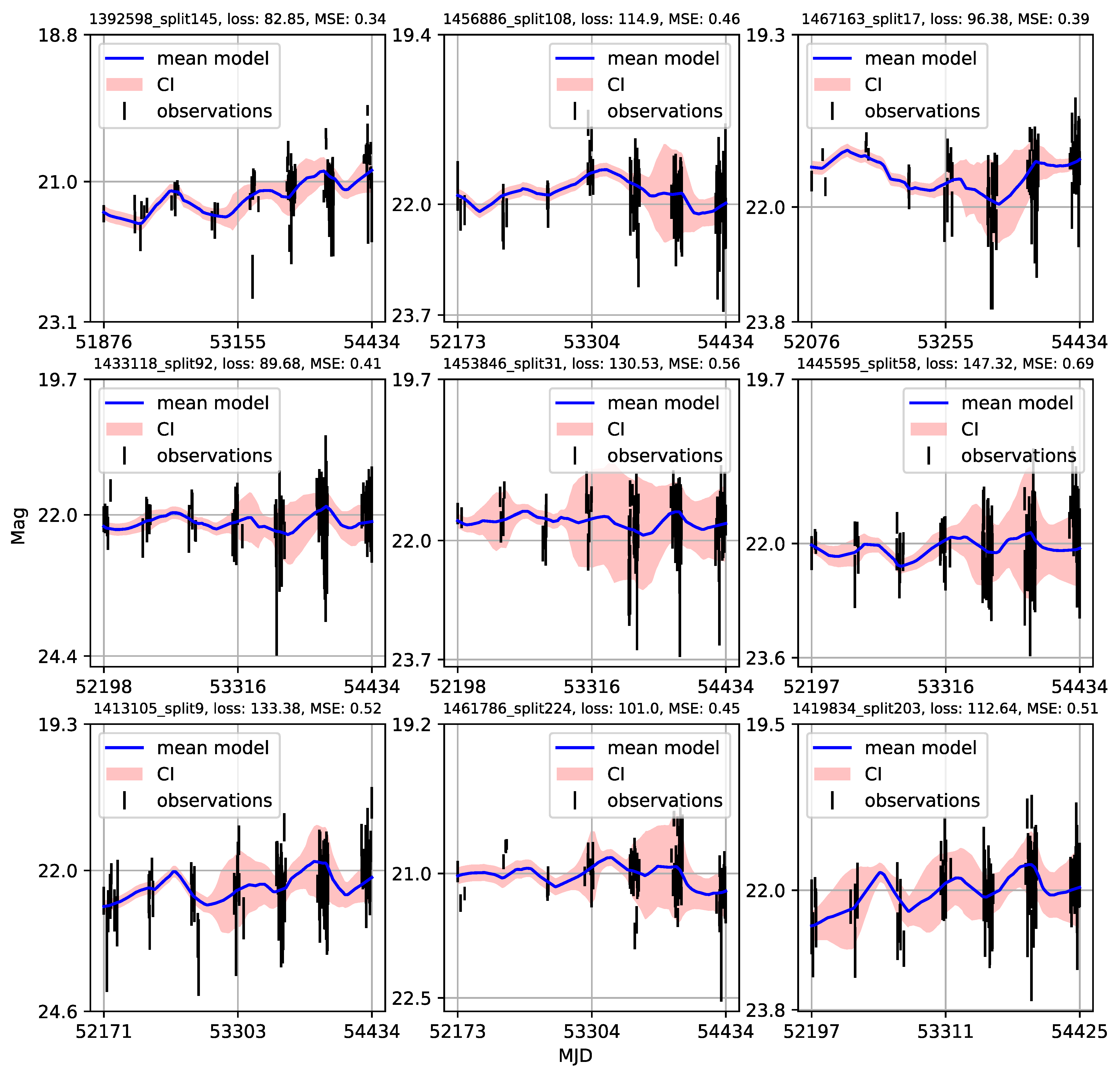
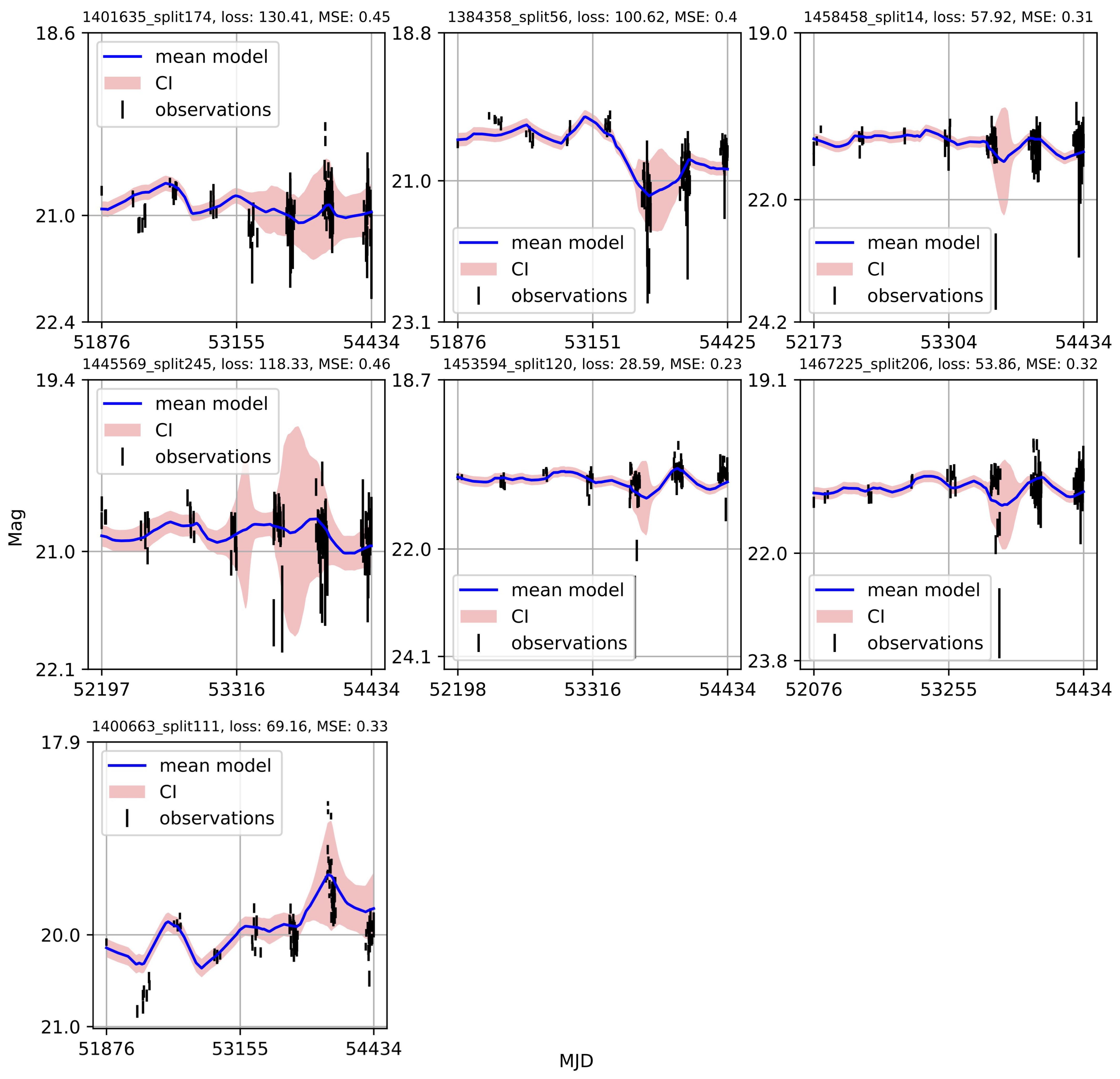
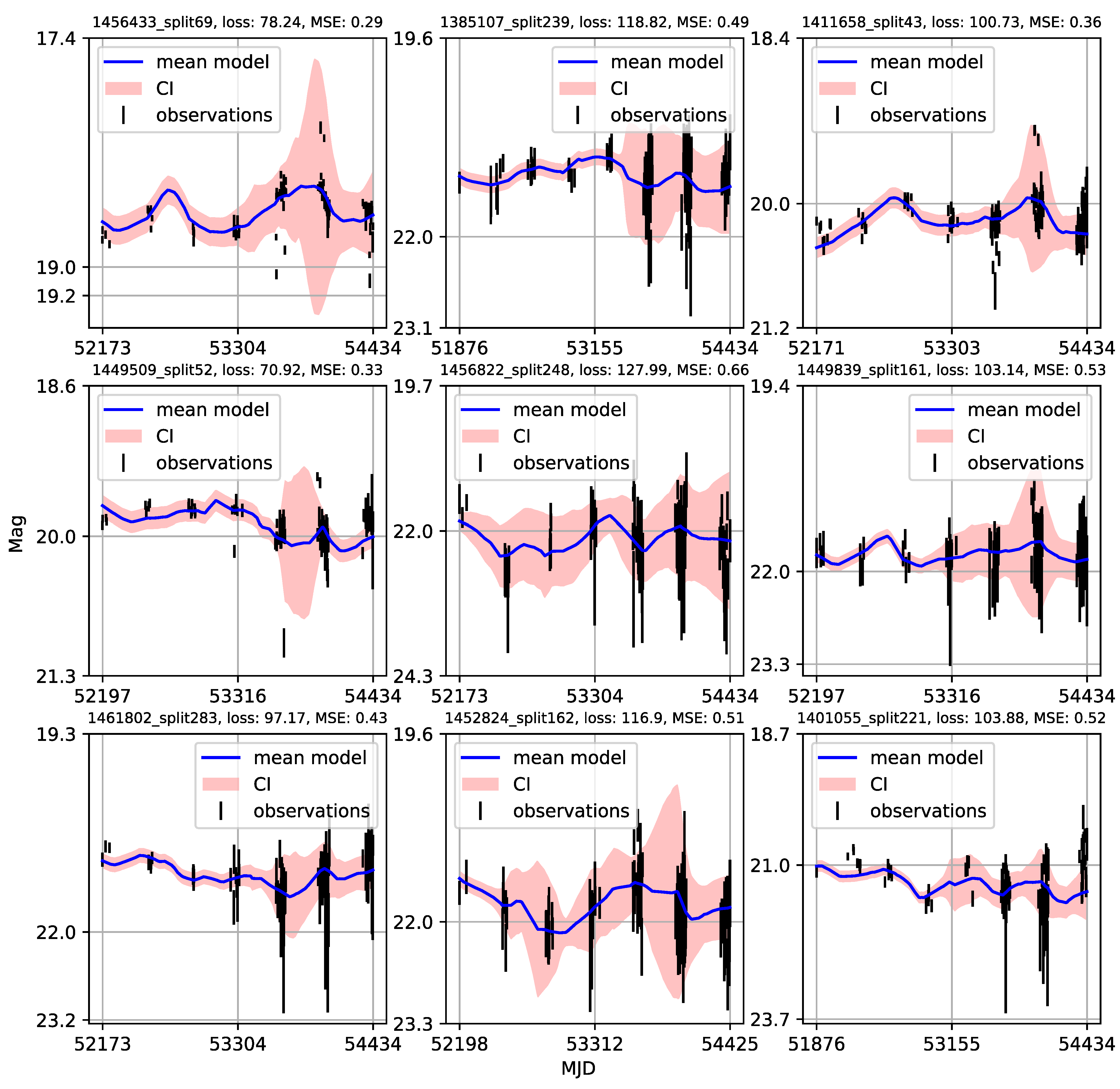
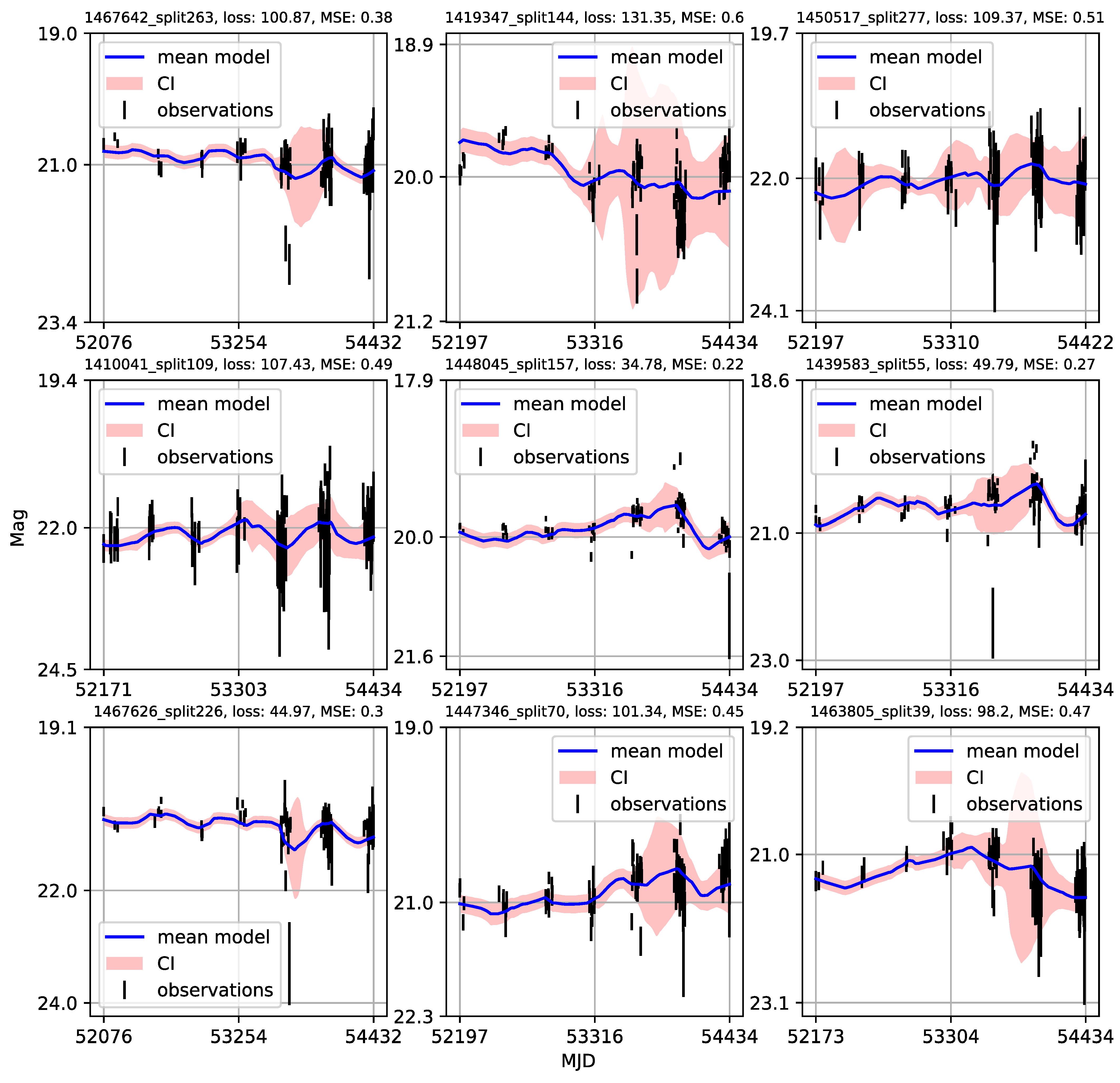
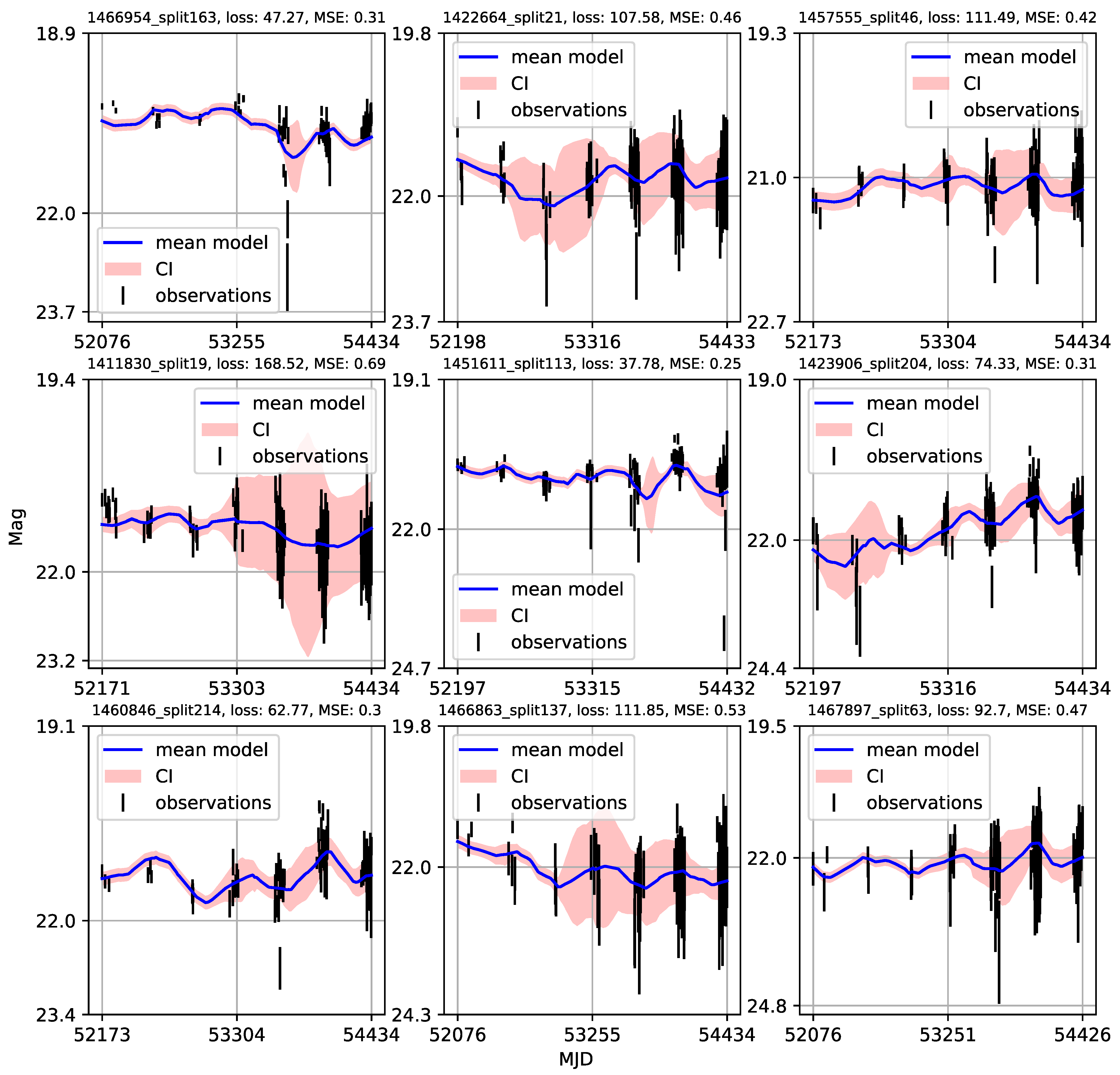
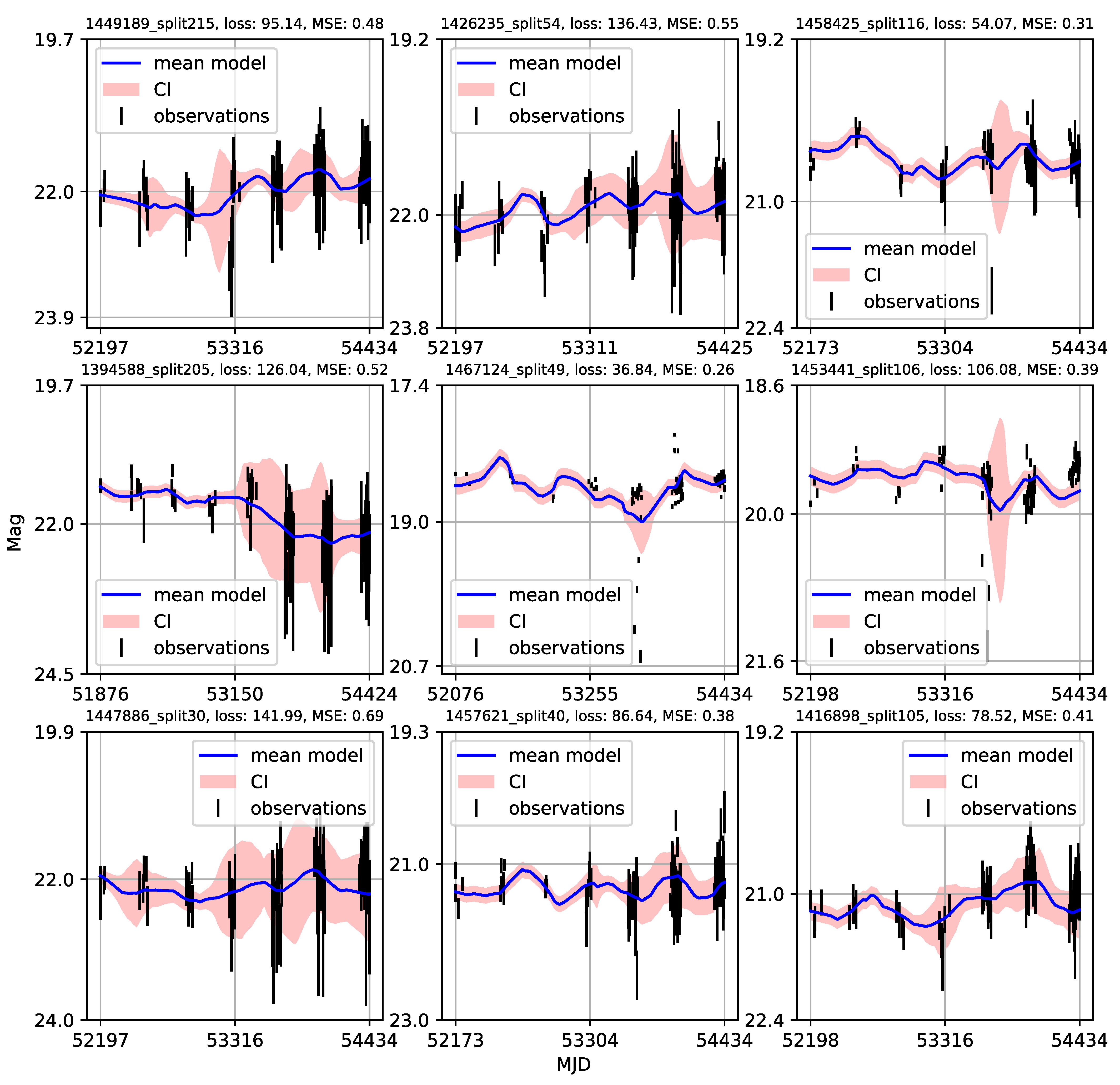
4.2. CNP Modeling of Quasar Variability

A detailed catalog of CNP models of light curves in our sample of 283 low variable and high redshift quasars ( F v a r 0.03 , 1 z 3 ) is given in the Appendix A (see Figure A1, Figure A2, Figure A3, Figure A4, Figure A5, Figure A6, Figure A7, Figure A8, Figure A9, Figure A10, Figure A11, Figure A12, Figure A13, Figure A14, Figure A15, Figure A16, Figure A17, Figure A18, Figure A19, Figure A20, Figure A21, Figure A22, Figure A23, Figure A24, Figure A25, Figure A26, Figure A27, Figure A28, Figure A29, Figure A30, Figure A31 and Figure A32). Each plot shows the modeling performance of the CNP. The most notable quality is that the CNP catches the overall trends and major flare-like events. Both the autoencoder neural network constructed by (compare to Figure 7 in Tachibana et al. [13]) and CNP model the quasar temporal behavior purely based on the characteristics of the data without any prior assumptions. However, the main difference is that CNP also inherits the flexibility of stochastic process modeling such as GP. To assess the modeling accuracy of the CNP each plot presents MSE and loss values along the 95 % confidence interval of the model. As we included observational errors in the CNP training process, the confidence bands for the regions of light curves dominated by points with larger errors are wider. Furthermore, we discovered that practically all light curves contain flare-like occurrences and even outliers, which also raise the obtained confidence band. We note that MSE is of comparable value to the MSE found in other studies (see, e.g., [67]). MSE is calculated on original (nontransformed data) and its value of ∼0.5 mag corresponds to ∼5%. Given that MSE represents variance, it is also more resistant to outliers (flares). Because loss is measured as the log of probability density, it is particularly susceptible to large gaps and outliers in our light curves. We emphasize that deep learning studies of astronomical time series report MSE (see [13,67]) frequently, so we will provide both MSE and loss.
The corner plot of mean square error, loss of each model fitting, and the corresponding mean magnitude and mean photometric error of observed light curves are given in Figure 7. According to the individual plots, a higher MSE (>0.5) is coupled with mean magnitudes in the range [20, 22] and mean photometric errors greater than 0.002. The tail of the marginal mean error distribution likewise contains these mean magnitudes.
In our previous analysis, CNP was applied to the light curves with significant changes of gradients, having inhomogeneous cadences and infrequent flare-like features [35]. However, as demonstrated in [68] and here, deeper analysis of flare-like patterns is needed. We are testing additional CNP alternatives, but we are treading carefully to avoid the unintended introduction of relations that do not exist in data (see [29]).

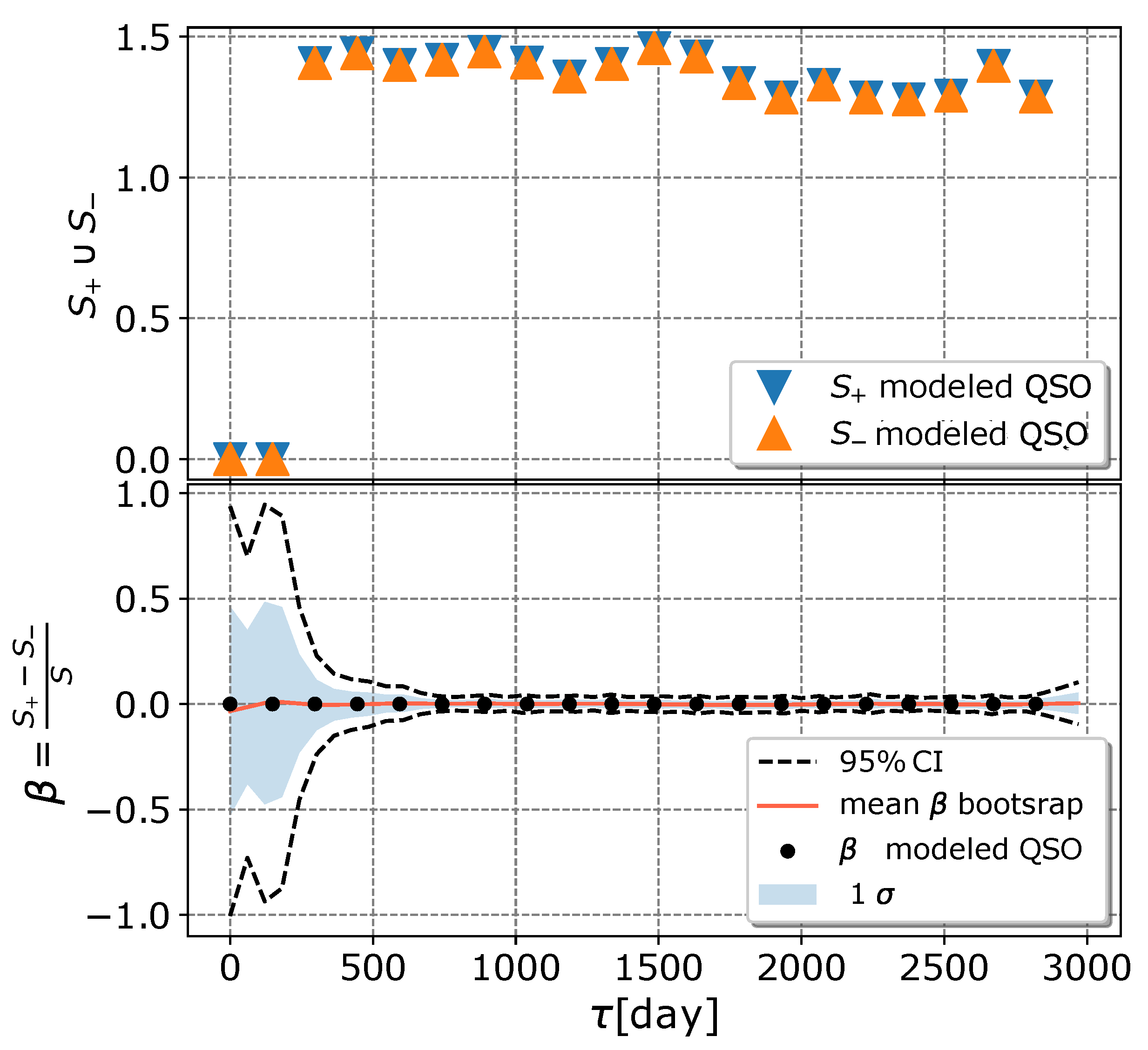
4.3. Modified Structure–Function Analysis of Observed and Modeled Light Curves

The results from the neural network clustering suggest that there is no significant variability in the quasar light curves of the chosen sample. In order to test and further investigate this finding, we used the structure functions (SF, see, e.g., [14,68,69] and references therein). The SF could be defined as [70]:  
S ( τ ) = 1 N ( τ ) i < j ( m ( t j ) m ( t i ) ) 2
where m ( t i ) is the magnitude measured at the epoch t i , and summation runs across the N ( τ ) epochs for which is satisfied t j t i = τ . In addition to S defined above, we also use the two modified structure functions S + and S introduced by Kawaguchi et al. [14]. For S + , the integration only includes pairings of magnitudes for which the flux increases m ( t j ) m ( t i ) > 0 , whereas for S , the integration only includes pairs of magnitudes for which the flux becomes dimmer m ( t j ) m ( t i ) < 0 .
Both modified structure functions measure the underlying asymmetry of the emission process as manifested in the light curves [14]. A comparison of modified structure functions could, in fact, disclose distinct mechanisms that are responsible for the variability of light curves, as was indicated in Hawkins [70]. To be more specific, the disc instability model shows itself in the form of an asymmetry in the light curves, such that the relation S > S + is observed at shorter time scales τ . On the other hand, transient events such as supernovae show up as the case that S + > S as the time scale gets shorter. In the scenario of microlensing, which is a fundamentally symmetrical process in the setting of quasar variability, the two functions are indistinguishable, denoted by the equation, i.e.,  S = S + [70]. Even though it looks paradoxical for quasars, Hawkins [70] explained this with a model where the fluctuations in the light curves originating from the accretion disc become smaller with increasing luminosity, while the effects of microlensing become more pronounced at higher redshift, which for quasars typically means higher luminosity.
Figure 8 displays S + and S , and  their relative difference normalized by standard SF (S, bottom panel) for observed quasar sample. Because of the regularity of large seasonal gaps in the observations, we were able to partition the data into five distinct time bins. In the top panel, both modified functions S + and S overlap. The normalized relative difference between them is also consistent with time symmetry.
The striking feature of both modified structure functions is their zero value at the time lag of around 800 days. Going back to the overview plot of observed light curves in Figure 3, we could see that this time lag comprises combinations of vertical columns of data points after M J D = 52,000 such as the first and third vertical, the second and fourth, the third and the sixth, etc., which are more similar in variability than other combinations that could be made. Moreover, we note that in the range 52,000 M J D 53,500 is an evidently smaller number of data points than for M J D > 52,500, which affects the bootstrapping method as it has larger uncertainty.
We can further compare the CNP-modeled light curves of the selected quasar sample by testing for time asymmetries (see Figure 9). It is important to note that modeled light curves made it possible to construct structure functions using a finer bin grid that contained 20 bins. As we have seen, S + and S of modeled light curves are practically identical, which lends further support to the idea that microlensing is at play here. We can see that the CNP modeling does not modify the fundamental variability characteristics of the light curves that have been observed.
For the structure functions of modeled light curves, the variability in the shortest timescale (<200 days) appears very different from that at a longer scale. This is an inevitable consequence of the fact that CNP is more uncertain about time lags corresponding to cadence gaps at epochs < 52,700 (see Figure 3 and Figure A1, Figure A2, Figure A3, Figure A4, Figure A5, Figure A6, Figure A7, Figure A8, Figure A9, Figure A10, Figure A11, Figure A12, Figure A13, Figure A14, Figure A15, Figure A16, Figure A17, Figure A18, Figure A19, Figure A20, Figure A21, Figure A22, Figure A23, Figure A24, Figure A25, Figure A26, Figure A27, Figure A28, Figure A29, Figure A30, Figure A31 and Figure A32). We could also see that the structure function’s confidence interval is rather large for these time lags.
We bring attention to the fact that our quasar sample was selected by our neural network algorithm in the absence of any other criteria (e.g., quasar parameter relationships), and that our clustering method based on the SOM could segregate objects with specific variability characteristics.
It is worth mentioning that microlensing can become obvious in multiple lensed quasar. This happens when some variations can only be observed in one image and appear to predominate over fluctuations that can be seen in all images over lengthy time scales. The light curves that are produced by microlensing can be simulated in a variety of different ways. Especially relevant to our collection of light curves are some interesting simulations by Lewis et al. [71]. In microlensing simulations, the source size has a significant impact on the look of the light curves, which become smoother and more rounded as the source size increases [70,71]. Light curves of our quasar sample given in Figure A1, Figure A2, Figure A3, Figure A4, Figure A5, Figure A6, Figure A7, Figure A8, Figure A9, Figure A10, Figure A11, Figure A12, Figure A13, Figure A14, Figure A15, Figure A16, Figure A17, Figure A18, Figure A19, Figure A20, Figure A21, Figure A22, Figure A23, Figure A24, Figure A25, Figure A26, Figure A27, Figure A28, Figure A29, Figure A30, Figure A31 and Figure A32 share a striking similarity with Figures 2a and 3b from Lewis et al. [71] regarding dominating non-smoothed flare-like patterns.
According to the findings of Tachibana et al. [13], modified structure functions and β ( τ ) for their sample of observed quasars exhibit asymmetry. They also noted that their simulated light curves as damped random walk (DRW) processes do not exhibit any substantial deviation from symmetric processes when compared to the bounds of confidence intervals. On the other hand, when we move deeper into the confidence interval, the values of the modified structure functions and β ( τ ) begin to fluctuate. Additionally, their simulated DRW light curves do not reflect the many flare-like events along the time baseline of light curves that are observed in our sample.
Based on the face value of these results, we find that the photometric variability of this sample of quasars could be explained with the microlensing model [70]. A justification that might be called is a model in which the fluctuations in the emission coming from the accretion disc becomes smaller as the luminosity of the object increases, but the effects of microlensing become more pronounced at higher redshifts, which for quasars typically coincide with higher luminosities (see [70]). We also note that low variability corresponds to high bolometric luminosity. The bolometric quasar luminosity is closely tied to the accretion rate of the SMBH. A bolometric quasar luminosity function (QLF) was constructed by Hopkins et al. [72] and updated for the bolometric QLF at z = 0 7 by Shen et al. [73].
Importantly, the flare-like patterns remained present in g and r curves (see an example in Figure 10). This is a hint that the flare-like events are achromatic since the gravitational bending of light is independent of the frequency of the radiation [74].
Nonetheless, it may be too soon to conclude that microlensing is the only plausible explanation. This is due to the fact that photometric monitoring for a period of four years is not yet sufficient to construct meaningful statistics based on the cadences that are available. Extreme optical extragalactic transients caused by explosion of supernovae, tidal disruption events around dormant black holes, rare blazars, stellar-mass black hole mergers in quasars disks, and intrinsic accretion outbursts in quasars may also be possible mechanisms behind observed flares (see [75]).
The discovery of such a distinct cluster of quasars in the LSST AGN data challenge database that makes ∼0.8% could have interesting implications.
Assuming that the LSST will harvest n O ( 2 × 10 7 10 8 ) quasars (see [23] and references therein), a very simple extrapolation indicates that future LSST data releases may contain a population of microlensed quasars that is not negligible ( N O ( 10 5 10 6 ) ). Interestingly, the microlensing duration should be shorter in the X-ray (several months) than in the UV/optical emission range [several years, see [76]). Moreover, cosmologically distributed lens objects may contribute significantly to the X-ray variability of high-redshifted QSOs ( z > 2 , [16]). Moreover, we could estimate N assuming the microlensing rate Γ , i.e., the number of events expected to be detected per quasar and per year. Γ was evaluated for particular quasar J1249+3449 as Γ 2 × 10 4 ( m / 0.1 M ) 0.5 events per quasar per year, where m is the lens mass (see [74]). The value of parameter m could be in the range of ( 0.01 0.5 ) M , if the host galaxy of quasar has stars with velocities 200–400  km s 1 , and a source lens distance in the range 1–10 kpc. Even if we caution that Γ was derived for a particular AGN [74], we could use it as a proxy to estimate within a time interval Δ t the total number N of expected microlensing events as simply N ϵ Γ t o t a l Δ t (see [77]). For simplicity, we assume that for maximal survey efficiency ϵ 1 , if n sources are monitored over a time interval Δ t the total rate is Γ t o t a l n × Γ . For  Δ t , we could expect to be within the range of weeks up to decades [78]. For example, Hawkins [15] found that if a lower limit of the time scale of ∼24 years was supposed to be caused by microlensing, it would correspond to a minimum mass for microlensing bodies of 0.4 M [15]. Taking into account that S + and S are more certain in our study for time scales >800 days, and since the LSST operation time is ∼10 yr, we estimated that the number of microlensing quasars in the LSST data releases may be N O ( 10 4 10 5 ) . Because of these assumptions, our estimates are most likely an upper bound on the number of microlensing quasars produced by LSST.
Nonetheless, in order to extract the physical properties of variability, the microlensing quasar population should be handled independently during the analysis process of the LSST quasar data, particularly the detection of binary candidates. Furthermore, it is probable that this population will have an influence on how quasars are classified in the LSST data pipelines.

5. Conclusions

In this follow-up study, we presented an improved version of a conditional neural process (CNP, Paper I) that was embedded in a multi-step approach for learning (stratification of light curves via neural network, deep learning of each stratum, statistical analysis of observed and modeled light curves in each stratum) from large amounts quasars contained in the LSST Active Galactic Nuclei Scientific Collaboration data challenge database. The main observations are:
  • Individual light curves of 1006 quasars having more than 100 epochs in LSST Active Galactic Nuclei Scientific Collaboration data challenge database exhibit a variety of behaviors, which can be generally stratified via the neural network into 36 clusters.
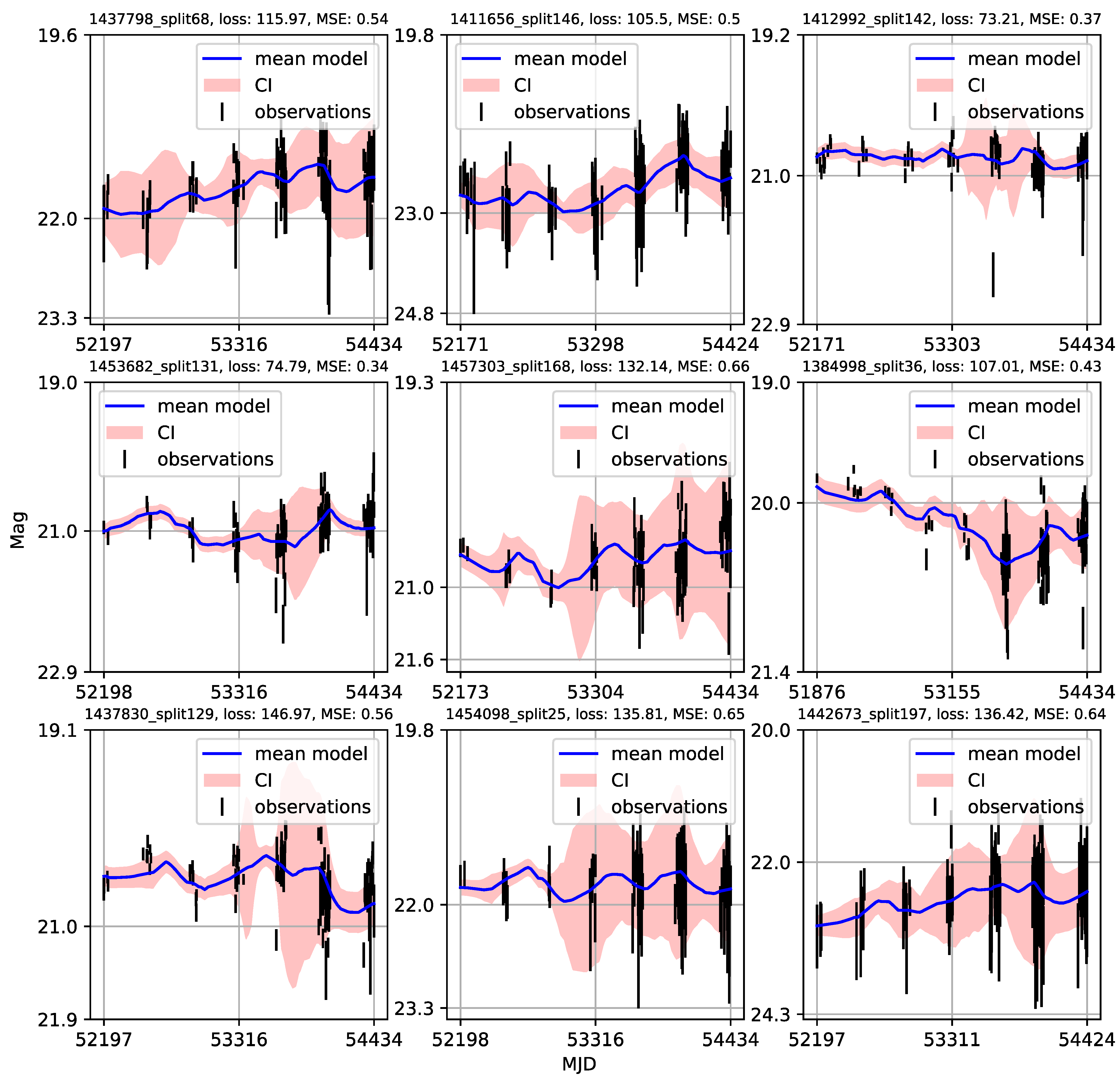
  • A case study of one of the stratified sets of u-band light curves for 283 quasars with very low variability F v a r 0.03 is presented here. The CNP model has an average mean square error of ∼5% (0.5 mag) on this stratum. Interestingly, all of the light curves in this stratum show features resembling the flares. An initial modified structure-function analysis suggests that these features may be linked to microlensing events that occur over longer time scales of five to ten years.
  • As many of the light curves in the LSST AGN data challenge database could be modeled with CNP, there are still enough objects having interesting features in the light curves (as our case study suggests) to urge a more extensive investigation.
With the help of this scientific case, we were also able to demonstrate the importance of CNP (along with other deep learning methods) for data-driven modeling in contexts where considerable samples of objects may have variability patterns that differ from the DRW. In the future, investigations of this nature should receive a greater amount of attention.

Author Contributions

Conceptualization, A.B.K., D.I., L.Č.P. and M.N.; LSST SER-SAG team members, L.Č.P., D.I., A.B.K. and M.N.; supervising and conceptualization of machine learning methodology, M.N., software design, M.N., A.B.K., N.A.M., I.Č.-H. and M.S.P.; supervising of mathematical analysis of light curves, M.K.; writing—original draft preparation, A.B.K., D.I., L.Č.P., M.S.P., M.N., N.A.M., I.Č.-H., M.K. and D.V.S., writing—review and editing, A.B.K., D.I., L.Č.P., M.S.P., M.N., N.A.M., I.Č.-H., M.K. and D.V.S. All authors have read and agreed to the published version of the manuscript.

Funding

A.B.K., D.I., L.Č.P., M.N. and M.K. acknowledge funding provided by University of Belgrade-Faculty of Mathematics (the contract №451-03-47/2023-01/200104), through the grants by the Ministry of Science, Technological Development and Innovation of the Republic of Serbia. A.B.K. and L.Č.P. thank the support by Chinese Academy of Sciences President’s International Fellowship Initiative (PIFI) for visiting scientist. L.Č.P. and D.V.S. acknowledges funding provided by Astronomical Observatory (the contract 451-03-68/2022-14/200002), through the grants by the Ministry of Education, Science, and Technological Development of the Republic of Serbia.

Data Availability Statement

The data are available from the corresponding author upon reasonable request and with the permission of the LSST AGN Scientific Collaboration.

Acknowledgments

We sincerely thank Gordon T. Richards, and  Weixiang Yu for their essential efforts in the construction of LSST AGN data challenge within the Rubin-LSST Science Collaborations. This work was conducted as a joint action of the Rubin-LSST Active Galactic Nuclei (AGN) and Transients and Variable Stars (TVS) Science Collaborations. The authors express their gratitude to the Vera C. Rubin LSST AGN and TVS Science Collaborations for fostering cooperation and the interchange of ideas and knowledge during their numerous meetings.

Conflicts of Interest

The authors declare no conflict of interest. The funders had no role in the design of the study; in the collection, analyses, or interpretation of data; in the writing of the manuscript; or in the decision to publish the results.

Abbreviations

    The following abbreviations are used in this manuscript:
AGNactive galactic nuclei
LSSTLegacy Survey of Space and Time
LSST_AGN_DCLSST AGN data challenge database
SMBHSupermassive black hole

Appendix A. Catalogue of CNP Models of u-Band Light Curves

Figure A1, Figure A2, Figure A3, Figure A4, Figure A5, Figure A6, Figure A7, Figure A8, Figure A9, Figure A10, Figure A11, Figure A12, Figure A13, Figure A14, Figure A15, Figure A16, Figure A17, Figure A18, Figure A19, Figure A20, Figure A21, Figure A22, Figure A23, Figure A24, Figure A25, Figure A26, Figure A27, Figure A28, Figure A29, Figure A30, Figure A31 and Figure A32 show a collection of plots of the observed u-band and corresponding predicted light curves for selected 283 objects using a training set for the CNP model.
Figure A1. CNP modeling of light curves. The subtitle of each plot shows the object ID from the LSST AGN DC database with a tag indicating the iteration when it is selected for training, testing, or validation during the training process, the logarithmic value of probability loss, and the MSE value. Black error bars indicate observations with measurement uncertainty. Solid blue lines are model fits to the data. The red band represents the 1 σ confidence interval.
Universe 09 00287 g0a1
Figure A2. CNP models of light curves. The subtitle of each plot shows the object ID from the LSST AGN DC database with a tag indicating the iteration when it is selected for training, testing, or validation during the training process, the logarithmic value of probability loss, and the MSE value. Black error bars indicate observations with measurement uncertainty. Solid blue lines are model fits to the data. The red band represents the 1 σ confidence interval.
Universe 09 00287 g0a2
Figure A3. CNP models of light curves. The subtitle of each plot shows the object ID from the LSST AGN DC database with a tag indicating the iteration when it is selected for training, testing, or validation during the training process, the logarithmic value of probability loss, and the MSE value. Black error bars indicate observations with measurement uncertainty. Solid blue lines are model fits to the data. The red band represents the 1 σ confidence interval.
Universe 09 00287 g0a3
Figure A4. CNP models of light curves. The subtitle of each plot shows the object ID from the LSST AGN DC database with a tag indicating the iteration when it is selected for training, testing, or validation during the training process, the logarithmic value of probability loss, and the MSE value. Black error bars indicate observations with measurement uncertainty. Solid blue lines are model fits to the data. The red band represents the 1 σ confidence interval.
Universe 09 00287 g0a4
Figure A5. CNP models of light curves. The subtitle of each plot shows the object ID from the LSST AGN DC database with a tag indicating the iteration when it is selected for training, testing, or validation during the training process, the logarithmic value of probability loss, and the MSE value. Black error bars indicate observations with measurement uncertainty. Solid blue lines are model fits to the data. The red band represents the 1 σ confidence interval.
Universe 09 00287 g0a5
Figure A6. CNP models of light curves. The subtitle of each plot shows the object ID from the LSST AGN DC database with a tag indicating the iteration when it is selected for training, testing, or validation during the training process, the logarithmic value of probability loss, and the MSE value. Black error bars indicate observations with measurement uncertainty. Solid blue lines are model fits to the data. The red band represents the 1 σ confidence interval.
Universe 09 00287 g0a6
Figure A7. CNP models of light curves. The subtitle of each plot shows the object ID from the LSST AGN DC database with a tag indicating the iteration when it is selected for training, testing, or validation during the training process, the logarithmic value of probability loss, and the MSE value. Black error bars indicate observations with measurement uncertainty. Solid blue lines are model fits to the data. The red band represents the 1 σ confidence interval.
Universe 09 00287 g0a7
Figure A8. CNP models of light curves. The subtitle of each plot shows the object ID from the LSST AGN DC database with a tag indicating the iteration when it is selected for training, testing, or validation during the training process, the logarithmic value of probability loss, and the MSE value. Black error bars indicate observations with measurement uncertainty. Solid blue lines are model fits to the data. The red band represents the 1 σ confidence interval.
Universe 09 00287 g0a8
Figure A9. CNP models of light curves. The subtitle of each plot shows the object ID from the LSST AGN DC database with a tag indicating the iteration when it is selected for training, testing, or validation during the training process, the logarithmic value of probability loss, and the MSE value. Black error bars indicate observations with measurement uncertainty. Solid blue lines are model fits to the data. The red band represents the 1 σ confidence interval.
Universe 09 00287 g0a9
Figure A10. CNP models of light curves. The subtitle of each plot shows the object ID from the LSST AGN DC database with a tag indicating the iteration when it is selected for training, testing, or validation during the training process, the logarithmic value of probability loss, and the MSE value. Black error bars indicate observations with measurement uncertainty. Solid blue lines are model fits to the data. The red band represents the 1 σ confidence interval.
Universe 09 00287 g0a10
Figure A11. CNP models of light curves. The subtitle of each plot shows the object ID from the LSST AGN DC database with a tag indicating the iteration when it is selected for training, testing, or validation during the training process, the logarithmic value of probability loss, and the MSE value. Black error bars indicate observations with measurement uncertainty. Solid blue lines are model fits to the data. The red band represents the 1 σ confidence interval.
Universe 09 00287 g0a11
Figure A12. CNP models of light curves. The subtitle of each plot shows the object ID from the LSST AGN DC database with a tag indicating the iteration when it is selected for training, testing, or validation during the training process, the logarithmic value of probability loss, and the MSE value. Black error bars indicate observations with measurement uncertainty. Solid blue lines are model fits to the data. The red band represents the 1 σ confidence interval.
Universe 09 00287 g0a12
Figure A13. CNP models of light curves. The subtitle of each plot shows the object ID from the LSST AGN DC database with a tag indicating the iteration when it is selected for training, testing, or validation during the training process, the logarithmic value of probability loss, and the MSE value. Black error bars indicate observations with measurement uncertainty. Solid blue lines are model fits to the data. The red band represents the 1 σ confidence interval.
Universe 09 00287 g0a13
Figure A14. CNP models of light curves. The subtitle of each plot shows the object ID from the LSST AGN DC database with a tag indicating the iteration when it is selected for training, testing, or validation during the training process, the logarithmic value of probability loss, and the MSE value. Black error bars indicate observations with measurement uncertainty. Solid blue lines are model fits to the data. The red band represents the 1 σ confidence interval.
Universe 09 00287 g0a14
Figure A15. CNP models of light curves. The subtitle of each plot shows the object ID from the LSST AGN DC database with a tag indicating the iteration when it is selected for training, testing, or validation during the training process, the logarithmic value of probability loss, and the MSE value. Black error bars indicate observations with measurement uncertainty. Solid blue lines are model fits to the data. The red band represents the 1 σ confidence interval.
Universe 09 00287 g0a15
Figure A16. CNP models of light curves. The subtitle of each plot shows the object ID from the LSST AGN DC database with a tag indicating the iteration when it is selected for training, testing, or validation during the training process, the logarithmic value of probability loss, and the MSE value. Black error bars indicate observations with measurement uncertainty. Solid blue lines are model fits to the data. The red band represents the 1 σ confidence interval.
Universe 09 00287 g0a16
Figure A17. CNP models of light curves. The subtitle of each plot shows the object ID from the LSST AGN DC database with a tag indicating the iteration when it is selected for training, testing, or validation during the training process, the logarithmic value of probability loss, and the MSE value. Black error bars indicate observations with measurement uncertainty. Solid blue lines are model fits to the data. The red band represents the 1 σ confidence interval.
Universe 09 00287 g0a17
Figure A18. CNP models of light curves. The subtitle of each plot shows the object ID from the LSST AGN DC database with a tag indicating the iteration when it is selected for training, testing, or validation during the training process, the logarithmic value of probability loss, and the MSE value. Black error bars indicate observations with measurement uncertainty. Solid blue lines are model fits to the data. The red band represents the 1 σ confidence interval.
Universe 09 00287 g0a18
Figure A19. CNP models of light curves. The subtitle of each plot shows the object ID from the LSST AGN DC database with a tag indicating the iteration when it is selected for training, testing, or validation during the training process, the logarithmic value of probability loss, and the MSE value. Black error bars indicate observations with measurement uncertainty. Solid blue lines are model fits to the data. The red band represents the 1 σ confidence interval.
Universe 09 00287 g0a19
Figure A20. CNP models of light curves. The subtitle of each plot shows the object ID from the LSST AGN DC database with a tag indicating the iteration when it is selected for training, testing, or validation during the training process, the logarithmic value of probability loss, and the MSE value. Black error bars indicate observations with measurement uncertainty. Solid blue lines are model fits to the data. The red band represents the 1 σ confidence interval.
Universe 09 00287 g0a20
Figure A21. CNP models of light curves. The subtitle of each plot shows the object ID from the LSST AGN DC database with a tag indicating the iteration when it is selected for training, testing, or validation during the training process, the logarithmic value of probability loss, and the MSE value. Black error bars indicate observations with measurement uncertainty. Solid blue lines are model fits to the data. The red band represents the 1 σ confidence interval.
Universe 09 00287 g0a21
Figure A22. CNP models of light curves. The subtitle of each plot shows the object ID from the LSST AGN DC database with a tag indicating the iteration when it is selected for training, testing, or validation during the training process, the logarithmic value of probability loss, and the MSE value. Black error bars indicate observations with measurement uncertainty. Solid blue lines are model fits to the data. The red band represents the 1 σ confidence interval.
Universe 09 00287 g0a22
Figure A23. CNP models of light curves. The subtitle of each plot shows the object ID from the LSST AGN DC database with a tag indicating the iteration when it is selected for training, testing, or validation during the training process, the logarithmic value of probability loss, and the MSE value. Black error bars indicate observations with measurement uncertainty. Solid blue lines are model fits to the data. The red band represents the 1 σ confidence interval.
Universe 09 00287 g0a23
Figure A24. CNP models of light curves. The subtitle of each plot shows the object ID from the LSST AGN DC database with a tag indicating the iteration when it is selected for training, testing, or validation during the training process, the logarithmic value of probability loss, and the MSE value. Black error bars indicate observations with measurement uncertainty. Solid blue lines are model fits to the data. The red band represents the 1 σ confidence interval.
Universe 09 00287 g0a24
Figure A25. CNP models of light curves. The subtitle of each plot shows the object ID from the LSST AGN DC database with a tag indicating the iteration when it is selected for training, testing, or validation during the training process, the logarithmic value of probability loss, and the MSE value. Black error bars indicate observations with measurement uncertainty. Solid blue lines are model fits to the data. The red band represents the 1 σ confidence interval.
Universe 09 00287 g0a25
Figure A26. CNP models of light curves. The subtitle of each plot shows the object ID from the LSST AGN DC database with a tag indicating the iteration when it is selected for training, testing, or validation during the training process, the logarithmic value of probability loss, and the MSE value. Black error bars indicate observations with measurement uncertainty. Solid blue lines are model fits to the data. The red band represents the 1 σ confidence interval.
Universe 09 00287 g0a26
Figure A27. CNP models of light curves. The subtitle of each plot shows the object ID from the LSST AGN DC database with a tag indicating the iteration when it is selected for training, testing, or validation during the training process, the logarithmic value of probability loss, and the MSE value. Black error bars indicate observations with measurement uncertainty. Solid blue lines are model fits to the data. The red band represents the 1 σ confidence interval.
Universe 09 00287 g0a27
Figure A28. CNP models of light curves. The subtitle of each plot shows the object ID from the LSST AGN DC database with a tag indicating the iteration when it is selected for training, testing, or validation during the training process, the logarithmic value of probability loss, and the MSE value. Black error bars indicate observations with measurement uncertainty. Solid blue lines are model fits to the data. The red band represents the 1 σ confidence interval.
Universe 09 00287 g0a28
Figure A29. CNP models of light curves. The subtitle of each plot shows the object ID from the LSST AGN DC database with a tag indicating the iteration when it is selected for training, testing, or validation during the training process, the logarithmic value of probability loss, and the MSE value. Black error bars indicate observations with measurement uncertainty. Solid blue lines are model fits to the data. The red band represents the 1 σ confidence interval.
Universe 09 00287 g0a29
Figure A30. CNP models of light curves. The subtitle of each plot shows the object ID from the LSST AGN DC database with a tag indicating the iteration when it is selected for training, testing, or validation during the training process, the logarithmic value of probability loss, and the MSE value. Black error bars indicate observations with measurement uncertainty. Solid blue lines are model fits to the data. The red band represents the 1 σ confidence interval.
Universe 09 00287 g0a30
Figure A31. CNP models of light curves. The subtitle of each plot shows the object ID from the LSST AGN DC database with a tag indicating the iteration when it is selected for training, testing, or validation during the training process, the logarithmic value of probability loss, and the MSE value. Black error bars indicate observations with measurement uncertainty. Solid blue lines are model fits to the data. The red band represents the 1 σ confidence interval.
Universe 09 00287 g0a31
Figure A32. CNP models of light curves. The subtitle of each plot shows the object ID from the LSST AGN DC database with a tag indicating the iteration when it is selected for training, testing, or validation during the training process, the logarithmic value of probability loss, and the MSE value. Black error bars indicate observations with measurement uncertainty. Solid blue lines are model fits to the data. The red band represents the 1 σ confidence interval.
Universe 09 00287 g0a32

Notes

1
Gaining knowledge from large astronomical databases is a complex procedure, including various deep learning algorithms and procedures so we will use ’deep learning’ in that wide context.
2
SER-SAG is Serbian team that contributes to AGN investigation and participates in the LSST AGN Scientific Collaboration
3
F v a r behaves as normalized variance so it is more robust to outliers, flares
4
We underline the distinction between NPs and both classic neural networks and GPs previously applied to quasars’ light curves. Classical neural network fit a single model across points based on learning from a large data collection, whereas GP fits a distribution of curves to a single set of observations (i.e., one light curve). NP combines both approaches, taking use of neural network ability to train on a large collection and GP’s ability to fit the distribution of curves because it is a metalearner.
5
In neural processes, the predicted distribution over functions is typically a Gaussian distribution, parameterized by a mean and variance.
6
We will use a subscript θ to denote all the parameters of the neural network such as number of layers, learning rate, size of batches, etc.
7
An assumption on P is that all finite sets of function evaluations of f are jointly Gaussian distributed. This class of random functions are known as Gaussian Processes (GPs).
8
We note that the our loss function works quite similarly to the Cross-Entropy. In the PyTorch ecosystem, Cross-Entropy Loss is obtained by combining a log-softmax layer and loss.
9
Data were transformed using min-max scaler adapted to the range a , b
scaled _ value = ( original _ value original _ min _ value ) × ( b a ) original _ max _ value original _ min _ value + a
where a = 2 ,   b = 2 and original _ value stands for the input data (time instances, magnitudes, magnitudes errors), original _ max _ value is the maximum of the original _ value , and  original _ min _ value is the minimum of the original _ value . This linear transformation (or more precisely affine) preserves the original distribution of data, does not reduce the importance of outliers, and preserves the covariance structure of the data. We used the range of 2 , 2 for enabling direct comparisons with [33] original testing data, ensuring consistency in our analysis.
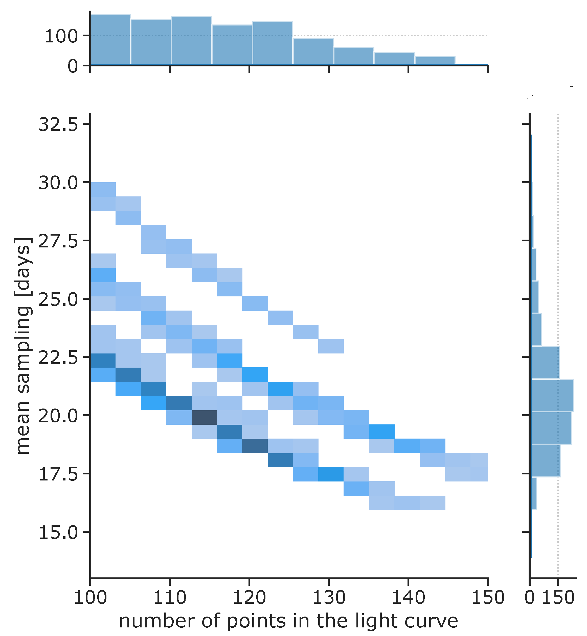
10
The N is the maximum number of points in the light curves in the given batch; missing values are zeropadded for shorter light curves. We emphasize that our sample of light curves is well balanced as a result of SOM clustering (see for an counter example [58]), so that the number of points per light curve covers a fairly limited range [103, 127] points, requiring negligible padding.

References

  1. Ivezić, Ž.; Kahn, S.M.; Tyson, J.A.; Abel, B.; Acosta, E.; Allsman, R.; Alonso, D.; AlSayyad, Y.; Anderson, S.F.; Andrew, J.; et al. LSST: From Science Drivers to Reference Design and Anticipated Data Products. Astrophys. J. 2019, 873, 111. [Google Scholar] [CrossRef]
  2. Anderson, S.F.; Haggard, D.; Homer, L.; Joshi, N.R.; Margon, B.; Silvestri, N.M.; Szkody, P.; Wolfe, M.A.; Agol, E.; Becker, A.C.; et al. Ultracompact AM Canum Venaticorum Binaries from the Sloan Digital Sky Survey: Three Candidates Plus the First Confirmed Eclipsing System. Astron. J. 2005, 130, 2230–2236. [Google Scholar] [CrossRef]
  3. Bloom, J.S.; Starr, D.L.; Butler, N.R.; Nugent, P.; Rischard, M.; Eads, D.; Poznanski, D. Towards a real-time transient classification engine. Astron. Nachr. 2008, 329, 284. [Google Scholar] [CrossRef] [Green Version]
  4. Scolnic, D.; Kessler, R.; Brout, D.; Cowperthwaite, P.S.; Soares-Santos, M.; Annis, J.; Herner, K.; Chen, H.Y.; Sako, M.; Doctor, Z.; et al. How Many Kilonovae Can Be Found in Past, Present, and Future Survey Data Sets? Astrophys. J. Lett. 2018, 852, L3. [Google Scholar] [CrossRef]
  5. Nuttall, L.K.; Berry, C.P.L. Electromagnetic counterparts of gravitational-wave signals. Astron. Geophys. 2021, 62, 4.15–4.21. [Google Scholar] [CrossRef]
  6. Kaspi, S.; Brandt, W.N.; Maoz, D.; Netzer, H.; Schneider, D.P.; Shemmer, O. Reverberation Mapping of High-Luminosity Quasars: First Results. Astrophys. J. 2007, 659, 997–1007. [Google Scholar] [CrossRef]
  7. MacLeod, C.L.; Ivezić, Ž.; Kochanek, C.S.; Kozłowski, S.; Kelly, B.; Bullock, E.; Kimball, A.; Sesar, B.; Westman, D.; Brooks, K.; et al. Modeling the Time Variability of SDSS Stripe 82 Quasars as a Damped Random Walk. Astrophys. J. 2010, 721, 1014–1033. [Google Scholar] [CrossRef] [Green Version]
  8. Graham, M.J.; Djorgovski, S.G.; Drake, A.J.; Mahabal, A.A.; Chang, M.; Stern, D.; Donalek, C.; Glikman, E. A novel variability-based method for quasar selection: Evidence for a rest-frame ∼54 d characteristic time-scale. Mon. Not. R. Astron. Soc. 2014, 439, 703–718. [Google Scholar] [CrossRef] [Green Version]
  9. Chapline, G.F.; Frampton, P.H. A new direction for dark matter research: Intermediate-mass compact halo objects. J. Cosmol. Astropart. Phys. 2016, 2016, 042. [Google Scholar] [CrossRef] [Green Version]
  10. Burke, C.J.; Shen, Y.; Blaes, O.; Gammie, C.F.; Horne, K.; Jiang, Y.F.; Liu, X.; McHardy, I.M.; Morgan, C.W.; Scaringi, S.; et al. A characteristic optical variability time scale in astrophysical accretion disks. Science 2021, 373, 789–792. [Google Scholar] [CrossRef]
  11. Risaliti, G.; Lusso, E. A Hubble Diagram for Quasars. Astrophys. J. 2015, 815, 33. [Google Scholar] [CrossRef]
  12. Marziani, P.; Dultzin, D.; del Olmo, A.; D’Onofrio, M.; de Diego, J.A.; Stirpe, G.M.; Bon, E.; Bon, N.; Czerny, B.; Perea, J.; et al. The quasar main sequence and its potential for cosmology. Proc. Nucl. Act. Galaxies Cosm. Time 2021, 356, 66–71. [Google Scholar] [CrossRef]
  13. Tachibana, Y.; Graham, M.J.; Kawai, N.; Djorgovski, S.G.; Drake, A.J.; Mahabal, A.A.; Stern, D. Deep Modeling of Quasar Variability. Astrophys. J. 2020, 903, 54. [Google Scholar] [CrossRef]
  14. Kawaguchi, T.; Mineshige, S.; Umemura, M.; Turner, E.L. Optical Variability in Active Galactic Nuclei: Starbursts or Disk Instabilities? Astrophys. J. 1998, 504, 671–679. [Google Scholar] [CrossRef]
  15. Hawkins, M.R.S. Timescale of variation and the size of the accretion disc in active galactic nuclei. Astron. Astrophys. 2007, 462, 581–589. [Google Scholar] [CrossRef] [Green Version]
  16. Zakharov, F.; Popović, L.Č.; Jovanović, P. On the contribution of microlensing to X-ray variability of high-redshifted QSOs. Astron. Astrophys. 2004, 420, 881–888. [Google Scholar] [CrossRef] [Green Version]
  17. Kelly, B.C.; Bechtold, J.; Siemiginowska, A. Are the variations in quasar optical flux driven by thermal fluctuations? Astrophys. J. 2009, 698, 895. [Google Scholar] [CrossRef]
  18. Sesar, B.; Ivezić, Ž.; Lupton, R.H.; Jurić, M.; Gunn, J.E.; Knapp, G.R.; DeLee, N.; Smith, J.A.; Miknaitis, G.; Lin, H.; et al. Exploring the Variable Sky with the Sloan Digital Sky Survey. Astron. J. 2007, 134, 2236–2251. [Google Scholar] [CrossRef] [Green Version]
  19. MacLeod, C.L.; Ivezić, Ž.; Sesar, B.; de Vries, W.; Kochanek, C.S.; Kelly, B.C.; Becker, A.C.; Lupton, R.H.; Hall, P.B.; Richards, G.T.; et al. A description of quasar variability measured using repeated sdss and poss imaging. Astrophys. J. 2012, 753, 106. [Google Scholar] [CrossRef]
  20. Kozłowski, S. Limitations on the recovery of the true AGN variability parameters using damped random walk modeling. Astron. Astrophys. 2017, 597, A128. [Google Scholar] [CrossRef] [Green Version]
  21. Kelly, B.C.; Becker, A.C.; Sobolewska, M.; Siemiginowska, A.; Uttley, P. Flexible and scalable methods for quantifying stochastic variability in the era of massive time-domain astronomical data sets. Astrophys. J. 2014, 788, 33. [Google Scholar] [CrossRef] [Green Version]
  22. Graham, M.J.; Djorgovski, S.G.; Drake, A.J.; Stern, D.; Mahabal, A.A.; Glikman, E.; Larson, S.; Christensen, E. Understanding extreme quasar optical variability with CRTS—I. Major AGN flares. Mon. Not. R. Astron. Soc. 2017, 470, 4112–4132. [Google Scholar] [CrossRef] [Green Version]
  23. Xin, C.; Haiman, Z. Ultra-short-period massive black hole binary candidates in LSST as LISA ‘verification binaries’. MNRAS 2021, 506, 2408–2417. [Google Scholar] [CrossRef]
  24. Amaro-Seoane, P.; Audley, H.; Babak, S.; Baker, J.; Barausse, E.; Bender, P.; Berti, E.; Binetruy, P.; Born, M.; Bortoluzzi, D.; et al. Laser Interferometer Space Antenna. arXiv 2017, arXiv:1702.00786. [Google Scholar] [CrossRef]
  25. Haiman, Z.; Kocsis, B.; Menou, K. The Population of Viscosity- and Gravitational Wave-Driven Supermassive Black Hole Binaries among Luminous Active Galactic Nuclei. Astrophys. J. 2009, 700, 1952. [Google Scholar] [CrossRef] [Green Version]
  26. Emmanoulopoulos, D.; McHardy, I.M.; Papadakis, I.E. Generating artificial light curves: Revisited and updated. Mon. Not. R. Astron. Soc. 2013, 433, 907–927. [Google Scholar] [CrossRef] [Green Version]
  27. Kelly, B.C.; Treu, T.; Malkan, M.; Pancoast, A.; Woo, J.H. Active Galactic Nucleus Black Hole Mass Estimates in the Era of Time Domain Astronomy. Astrophys. J. 2013, 779, 187. [Google Scholar] [CrossRef] [Green Version]
  28. Mushotzky, R.F.; Edelson, R.; Baumgartner, W.; Gandhi, P. Kepler Observations of Rapid Optical Variability in Active Galactic Nuclei. Astrophys. J. Lett. 2011, 743, L12. [Google Scholar] [CrossRef] [Green Version]
  29. Smith, K.L.; Mushotzky, R.F.; Boyd, P.T.; Malkan, M.; Howell, S.B.; Gelino, D.M. The Kepler Light Curves of AGN: A Detailed Analysis. Astrophys. J. 2018, 857, 141. [Google Scholar] [CrossRef] [Green Version]
  30. Yu, W.; Richards, G.T.; Vogeley, M.S.; Moreno, J.; Graham, M.J. Examining AGN UV/Optical Variability beyond the Simple Damped Random Walk. Astrophys. J. 2022, 936, 132. [Google Scholar] [CrossRef]
  31. Zhang, S.Q.; Wang, F.; Fan, F.L. Neural Network Gaussian Processes by Increasing Depth. IEEE Trans. Neural Netw. Learn. Syst. 2022, 1–6. [Google Scholar] [CrossRef] [PubMed]
  32. Danilov, E.; Ćiprijanović, A.; Nord, B. Neural Inference of Gaussian Processes for Time Series Data of Quasars. arXiv 2022, arXiv:2211.10305. [Google Scholar] [CrossRef]
  33. Garnelo, M.; Schwarz, J.; Rosenbaum, D.; Viola, F.; Rezende, D.; Eslami, S.; Teh, Y. Neural Processes. In Proceedings of the Theoretical Foundations and Applications of Deep Generative Models Workshop, International Conference on Machine Learning (ICML), Stockholm, Sweden, 14–15 July 2018; pp. 1704, 1713. [Google Scholar]
  34. Yu, W.; Richards, G.; Buat, V.; Brandt, W.N.; Banerji, M.; Ni, Q.; Shirley, R.; Temple, M.; Wang, F.; Yang, J. LSSTC AGN Data Challenge 2021; Zenodo: Geneve, Switzerland, 2022. [Google Scholar] [CrossRef]
  35. Čvorović-Hajdinjak, I.; Kovačević, A.B.; Ilić, D.; Popović, L.Č.; Dai, X.; Jankov, I.; Radović, V.; Sánchez-Sáez, P.; Nikutta, R. Conditional Neural Process for nonparametric modeling of active galactic nuclei light curves. Astron. Nachr. 2022, 343, e210103. [Google Scholar] [CrossRef]
  36. Oguri, M.; Marshall, P.J. Gravitationally lensed quasars and supernovae in future wide-field optical imaging surveys. Mon. Not. R. Astron. Soc. 2010, 405, 2579–2593. [Google Scholar] [CrossRef] [Green Version]
  37. Neira, F.; Anguita, T.; Vernardos, G. A quasar microlensing light-curve generator for LSST. Mon. Not. R. Astron. Soc. 2020, 495, 544–553. [Google Scholar] [CrossRef]
  38. Savić, D.V.; Jankov, I.; Yu, W.; Petrecca, V.; Temple, M.; Ni, Q.; Shirley, R.; Kovačević, A.; Nikolić, M.; Ilić, D.; et al. The LSST AGN Data Challenge: Selection methods. Astrophys. J. 2022. submitted. [Google Scholar]
  39. Richards, J.W.; Starr, D.L.; Butler, N.R.; Bloom, J.S.; Brewer, J.M.; Crellin-Quick, A.; Higgins, J.; Kennedy, R.; Rischard, M. On Machine-learned Classification of Variable Stars with Sparse and Noisy Time-series Data. Astrophys. J. 2011, 733, 10. [Google Scholar] [CrossRef]
  40. Kovacevic, A.; Ilic, D.; Jankov, I.; Popovic, L.C.; Yoon, I.; Radovic, V.; Caplar, N.; Cvorovic-Hajdinjak, I. LSST AGN SC Cadence Note: Two metrics on AGN variability observable. arXiv 2021, arXiv:2105.12420. [Google Scholar] [CrossRef]
  41. Kovačević, A.B.; Radović, V.; Ilić, D.; Popović, L.Č.; Assef, R.J.; Sánchez-Sáez, P.; Nikutta, R.; Raiteri, C.M.; Yoon, I.; Homayouni, Y.; et al. The LSST Era of Supermassive Black Hole Accretion Disk Reverberation Mapping. Astrophys. J. Suppl. 2022, 262, 49. [Google Scholar] [CrossRef]
  42. Kasliwal, V.P.; Vogeley, M.S.; Richards, G.T. Are the variability properties of the Kepler AGN light curves consistent with a damped random walk? Mon. Not. R. Astron. Soc. 2015, 451, 4328–4345. [Google Scholar] [CrossRef] [Green Version]
  43. Vettigli, G. MiniSom: Minimalistic and NumPy-Based Implementation of the Self Organizing Map. 2018. Available online: https://github.com/JustGlowing/minisom (accessed on 8 June 2023).
  44. Edelson, R.A.; Krolik, J.H.; Pike, G.F. Broad-Band Properties of the CfA Seyfert Galaxies. III. Ultraviolet Variability. Astrophys. J. 1990, 359, 86. [Google Scholar] [CrossRef]
  45. Vaughan, S.; Edelson, R.; Warwick, R.S.; Uttley, P. On characterizing the variability properties of X-ray light curves from active galaxies. Mon. Not. R. Astron. Soc. 2003, 345, 1271–1284. [Google Scholar] [CrossRef]
  46. Solomon, R.; Stojkovic, D. Variability in quasar light curves: Using quasars as standard candles. J. Cosmol. Astropart. Phys. 2022, 2022, 060. [Google Scholar] [CrossRef]
  47. Condon, J.J.; Matthews, A.M. ΛCDM Cosmology for Astronomers. Publ. Astron. Soc. Pac. 2018, 130, 073001. [Google Scholar] [CrossRef] [Green Version]
  48. Planck Collaboration; Aghanim, N.; Akrami, Y.; Ashdown, M.; Aumont, J.; Baccigalupi, C.; Ballardini, M.; Banday, A.J.; Barreiro, R.B.; Bartolo, N.; et al. Planck 2018 results—VI. Cosmological parameters. Astron. Astrophys. 2020, 641, A6. [Google Scholar] [CrossRef] [Green Version]
  49. Rodrigo, C.; Solano, E.; Bayo, A. SVO Filter Profile Service, Version 1.0; IVOA Working Draft: València, Spain, 15 October 2012. [Google Scholar] [CrossRef]
  50. Rodrigo, C.; Solano, E. The SVO Filter Profile Service. In Proceedings of the XIV. 0 Scientific Meeting (Virtual) of the Spanish Astronomical Society, Virtual, 5–9 September 2020. [Google Scholar]
  51. Dexter, J.; Agol, E. Quasar Accretion Disks are Strongly Inhomogeneous. Astrophys. J. Lett. 2011, 727, L24. [Google Scholar] [CrossRef] [Green Version]
  52. Zu, Y.; Kochanek, C.S.; Kozłowski, S.; Udalski, A. Is Quasar Optical Variability a Damped Random Walk? Astrophys. J. 2013, 765, 106. [Google Scholar] [CrossRef]
  53. Caplar, N.; Lilly, S.J.; Trakhtenbrot, B. Optical Variability of AGNs in the PTF/iPTF Survey. Astrophys. J. 2017, 834, 111. [Google Scholar] [CrossRef]
  54. Ruan, J.J.; Anderson, S.F.; MacLeod, C.L.; Becker, A.C.; Burnett, T.H.; Davenport, J.R.A.; Ivezić, Ž.; Kochanek, C.S.; Plotkin, R.M.; Sesar, B.; et al. Characterizing the Optical Variability of Bright Blazars: Variability-based Selection of Fermi Active Galactic Nuclei. Astrophys. J. 2012, 760, 51. [Google Scholar] [CrossRef]
  55. Foong, A.; Bruinsma, W.; Gordon, J.; Dubois, Y.; Requeima, J.; Turner, R. Meta-learning stationary stochastic process prediction with convolutional neural processes. Adv. Neural Inf. Process. Syst. 2020, 33, 8284–8295. [Google Scholar]
  56. Tak, H.; Mandel, K.; Van Dyk, D.A.; Kashyap, V.L.; Meng, X.L.; Siemiginowska, A. Bayesian estimates of astronomical time delays between gravitationally lensed stochastic light curves. Ann. Appl. Stat. 2017, 13, 1309–1348. [Google Scholar] [CrossRef] [Green Version]
  57. Breivik, K.; Connolly, A.J.; Ford, K.E.S.; Jurić, M.; Mandelbaum, R.; Miller, A.A.; Norman, D.; Olsen, K.; O’Mullane, W.; Price-Whelan, A.; et al. From Data to Software to Science with the Rubin Observatory LSST. arXiv 2022, arXiv:2208.02781. [Google Scholar] [CrossRef]
  58. Sánchez-Sáez, P.; Lira, H.; Martí, L.; Sánchez-Pi, N.; Arredondo, J.; Bauer, F.E.; Bayo, A.; Cabrera-Vives, G.; Donoso-Oliva, C.; Estévez, P.A.; et al. Searching for Changing-state AGNs in Massive Data Sets. I. Applying Deep Learning and Anomaly-detection Techniques to Find AGNs with Anomalous Variability Behaviors. Astron. J. 2021, 162, 206. [Google Scholar] [CrossRef]
  59. Holmstrom, L.; Koistinen, P. Using additive noise in back-propagation training. IEEE Trans. Neural Netw. 1992, 3, 24–38. [Google Scholar] [CrossRef] [PubMed]
  60. Matsuoka, K. Noise injection into inputs in back-propagation learning. IEEE Trans. Syst. Man Cybern. 1992, 22, 436–440. [Google Scholar] [CrossRef]
  61. Bishop, C. Training with noise is equivalent to Tikhonov regularization. Neural Comput. 1995, 7, 108–116. [Google Scholar] [CrossRef]
  62. Wang, C.; Principe, J. Training neural networks with additive noise in the desired signal. IEEE Trans. Neural Netw. 1999, 10, 1511–1517. [Google Scholar] [CrossRef] [Green Version]
  63. Zur, R.M.; Jiang, Y.; Pesce, L.L.; Drukker, K. Noise injection for training artificial neural networks: A comparison with weight decay and early stopping. Med. Phys. 2009, 36, 4810–4818. [Google Scholar] [CrossRef] [Green Version]
  64. Goodfellow, I.; Bengio, Y.; Courville, A. Adaptive computation and machine learning. In Deep Learning; MIT Press: Cambridge, MA, USA, 2016. [Google Scholar]
  65. Zhang, X.; Yang, F.; Guo, Y.; Yu, H.; Wang, Z.; Zhang, Q. Adaptive Differential Privacy Mechanism Based on Entropy Theory for Preserving Deep Neural Networks. Mathematics 2023, 11, 330. [Google Scholar] [CrossRef]
  66. Reed, R.D.; Marks, R.J. Neural Smithing: Supervised Learning in Feedforward Artificial Neural Networks; MIT Press: Cambridge, MA, USA, 1998. [Google Scholar]
  67. Naul, B.; Bloom, J.S.; Pérez, F.; van der Walt, S. A recurrent neural network for classification of unevenly sampled variable stars. Nat. Astron. 2018, 2, 151–155. [Google Scholar] [CrossRef] [Green Version]
  68. Kasliwal, V.P.; Vogeley, M.S.; Richards, G.T.; Williams, J.; Carini, M.T. Do the Kepler AGN light curves need reprocessing? Mon. Not. R. Astron. Soc. 2015, 453, 2075–2081. [Google Scholar] [CrossRef] [Green Version]
  69. De Cicco, D.; Bauer, F.E.; Paolillo, M.; Sánchez-Sáez, P.; Brandt, W.N.; Vagnetti, F.; Pignata, G.; Radovich, M.; Vaccari, M. A structure function analysis of VST-COSMOS AGN. Astron. Astrophys. 2022, 664, A117. [Google Scholar] [CrossRef]
  70. Hawkins, M. Variability in active galactic nuclei: Confrontation of models with observations. Mon. Not. R. Astron. Soc. 2002, 329, 76–86. [Google Scholar] [CrossRef] [Green Version]
  71. Lewis, G.F.; Miralda-Escude, J.; Richardson, D.C.; Wambsganss, J. Microlensing light curves: A new and efficient numerical method. Mon. Not. R. Astron. Soc. 1993, 261, 647–656. [Google Scholar] [CrossRef] [Green Version]
  72. Hopkins, P.F.; Richards, G.T.; Hernquist, L. An Observational Determination of the Bolometric Quasar Luminosity Function. Astrophys. J. 2007, 654, 731. [Google Scholar] [CrossRef]
  73. Shen, X.; Hopkins, P.F.; Faucher-Giguère, C.A.; Alexander, D.M.; Richards, G.T.; Ross, N.P.; Hickox, R.C. The bolometric quasar luminosity function at z = 0–7. Mon. Not. R. Astron. Soc. 2020, 495, 3252–3275. [Google Scholar] [CrossRef]
  74. De Paolis, F.; Nucita, A.A.; Strafella, F.; Licchelli, D.; Ingrosso, G. A quasar microlensing event towards J1249+3449? Mon. Not. R. Astron. Soc. 2020, 499, L87–L90. [Google Scholar] [CrossRef]
  75. Graham, M.J.; McKernan, B.; Ford, K.E.S.; Stern, D.; Djorgovski, S.G.; Coughlin, M.; Burdge, K.B.; Bellm, E.C.; Helou, G.; Mahabal, A.A.; et al. A Light in the Dark: Searching for Electromagnetic Counterparts to Black Hole-Black Hole Mergers in LIGO/Virgo O3 with the Zwicky Transient Facility. Astrophys. J. 2023, 942, 99. [Google Scholar] [CrossRef]
  76. Jovanović, P.; Zakharov, A.F.; Popović, L.Č.; Petrović, T. Microlensing of the X-ray, UV and optical emission regions of quasars: Simulations of the time-scales and amplitude variations of microlensing events. Mon. Not. R. Astron. Soc. 2008, 386, 397–406. [Google Scholar] [CrossRef] [Green Version]
  77. Wang, J.; Smith, M.C. Using microlensed quasars to probe the structure of the Milky Way. Mon. Not. R. Astron. Soc. 2010, 410, 1135–1144. [Google Scholar] [CrossRef] [Green Version]
  78. Wambsganss, J. Microlensing of Quasars. Publ. Astron. Soc. Aust. 2001, 18, 207–210. [Google Scholar] [CrossRef] [Green Version]
Figure 2. Statistical description of 1006 quasar light curves in the u band having ≥100 points. The primary joint distribution plot of the number of points in the light curves and mean sampling makes the stratification of mean sampling very obvious. The non-Gaussianity of the mean sample and the number of points in the light curves are brought to light by the marginal distributions that are presented on the side plots. The marginals are presented as counts in this instance. Upper marginal: y-axis counts a number of light curves having a number of points given in x-axis in the main plot. Right marginal: y-axis counts a number of light curves having mean sampling in y-axis in the main plot.
Universe 09 00287 g002
Figure 3. Cluster of 283 u-band light curves with low variability obtained via SOM algorithm. Observed magnitudes are given as points, while solid lines serve as an eye guide. The magnitudes of each light curve have been multiplied by their ordinal number for clarity. Warmer colors correspond to higher ordinal numbers.
Universe 09 00287 g003
Figure 4. Corner plot of the probability distribution of quasars parameters in selected Cluster 36. Because the parameter distribution is multi-dimensional (only four are seen here), the information is unfolded into a succession of 1D and 2D representations. The histograms of the marginalized probability for each parameter are given on the diagonal. The scatter plots for all pairwise parameter combinations are given on the off-diagonal.
Universe 09 00287 g004
Figure 5. Forward pass (left to right) computational graph of the conditional neural process (see [55]). Contexts (observed points) are given in a red circle. MLP is a multilayer perceptron. R c is local encoding of context points, whereas R is general encoding. For given target time instances x t in a blue circle, the decoder, which is an MLP, produces the predictive distribution of the target output ( μ ( t ) , σ 2 ( t ) ) and predicted values y t .
Universe 09 00287 g005
Figure 6. Loss (the upper left panel), mean absolute error (MAE, the upper right panel) and MSE (the bottom left panel) for the training (orange) and for the validation (blue) data set during 100 runs of training. The dashed black lines represent the mean values of metrics at each epoch over 100 runs. Training loss is estimated in each iteration within each epoch, but validation loss is obtained at the end of each epoch. Inset plots show corresponding variances for training (orange) and validation (blue) data sets (a subset is shown for clarity). The metrics are expected to be high in the early epochs (since the network is initialized at random and the network’s behavior differs from the desired one in the early epochs). The behavior of metrics at a larger extent of epochs justifies the inclusion of early stopping criterion in the CNP.
Universe 09 00287 g006
Figure 7. Corner plot of the probability distribution of modeling parameters (MSE, loss) for corresponding observed light curves parameters (mean magnitude < m a g > , mean photometric error < σ > ). Histograms of the marginalized probability for each parameter are given on the diagonal.
Universe 09 00287 g007
Figure 8. Time symmetry in the light curves of selected quasar samples. Top: S and S + for the quasar sample are indicated by upward and downward pointing triangles, respectively. Bottom: The normalized relative difference β = S + S S for observed quasar sample (black dots), mean β (red line), 1 σ (blue band), and 95 % (dashed lines) confidence intervals as inferred from the bootstrapping quasar sample.
Universe 09 00287 g008
Figure 9. The same as Figure 8 but for CNP-modeled light curves.
Universe 09 00287 g009
Figure 10. Comparison of presence of flare-like patterns in u (black), g (green) and r (red) bands. Object identification number is given in the corresponding plot title.
Universe 09 00287 g010
Disclaimer/Publisher’s Note: The statements, opinions and data contained in all publications are solely those of the individual author(s) and contributor(s) and not of MDPI and/or the editor(s). MDPI and/or the editor(s) disclaim responsibility for any injury to people or property resulting from any ideas, methods, instructions or products referred to in the content.

