
Modeling the Topside Ionosphere Effective Scale Height through In Situ Electron Density Observations by Low-Earth-Orbit Satellites

 , ,
, ,  ,
,  , , ,
, , ,  ,
,  and
and 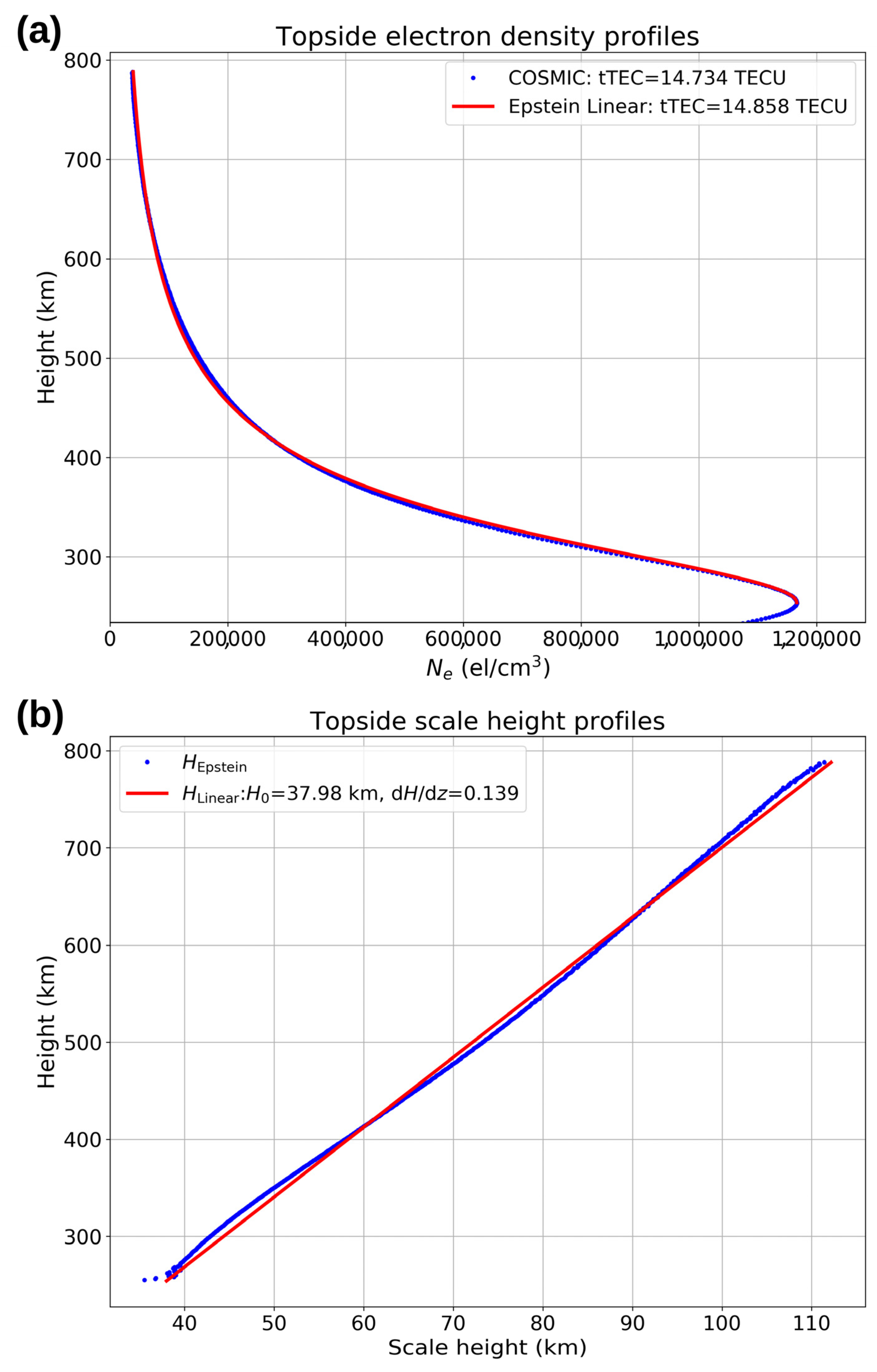
Abstract
1. Introduction
2. Data Description
2.1. CSES—01 Langmuir Probe Observations
2.2. Swarm B Langmuir Probe Observations
2.3. IRI F2-Layer Peak Modeled Characteristics
2.4. COSMIC/FORMOSAT—3 Radio Occultation Observations
3. Topside Effective Scale Height Calculation Methodology
3.1. NeQuick Model Topside Representation and Effective Scale Height Linear Approximation
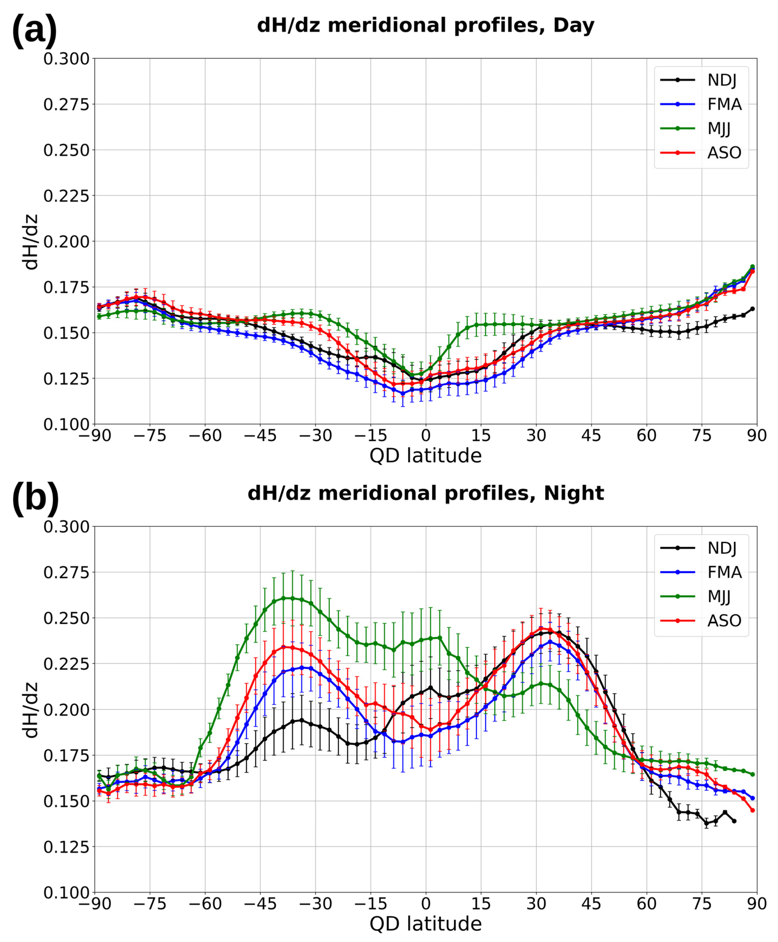
3.2. Topside Effective Scale Height Vertical Gradient Modeling
- NDJ: November, December, January—the months around the December solstice;
- FMA: February, March, April—the months around the March equinox;
- MJJ: May, June, July—the months around the June solstice;
- ASO: August, September, October—the months around the September equinox.
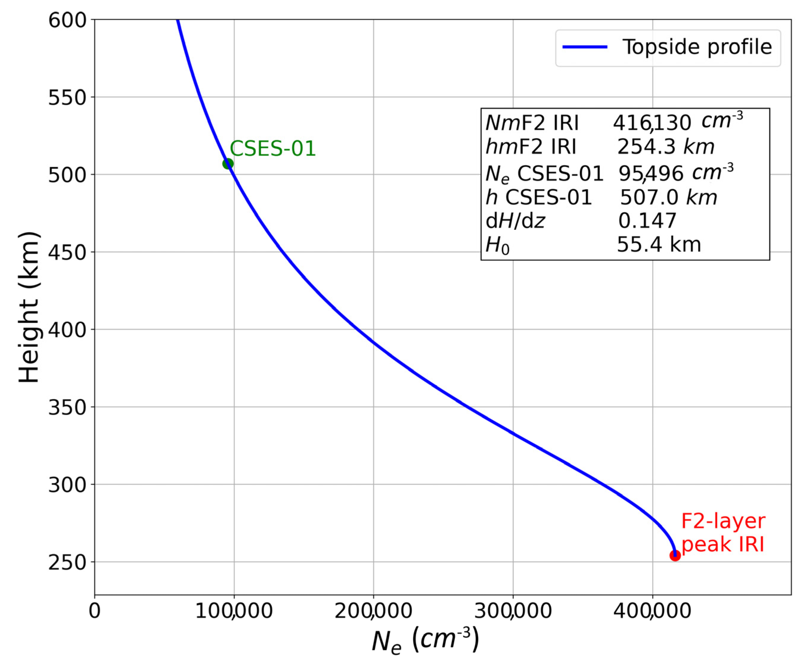
3.3. Modeling the Effective Scale Height at the F2-Layer Peak through In Situ LEO Ne Observations
4. Results
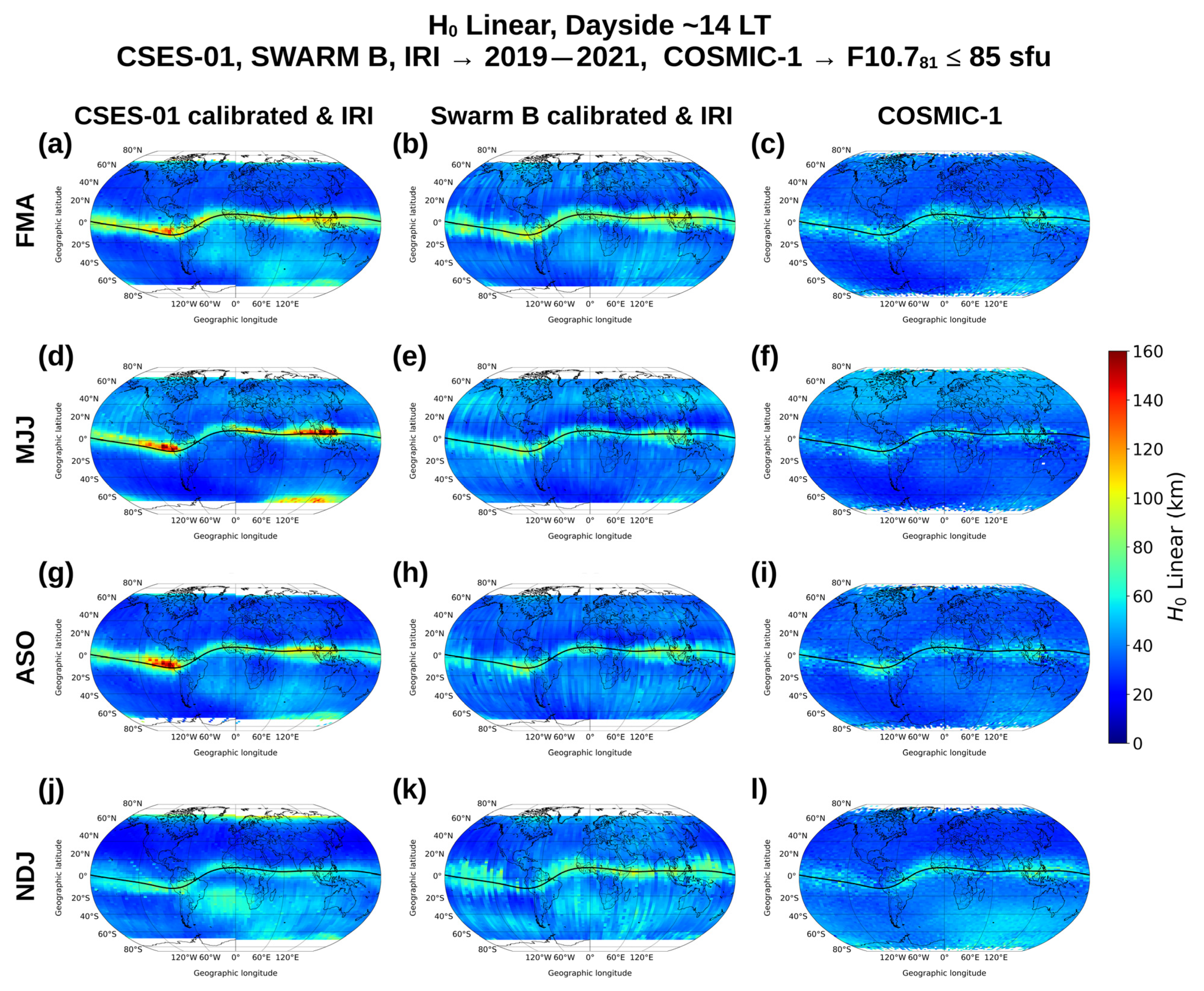
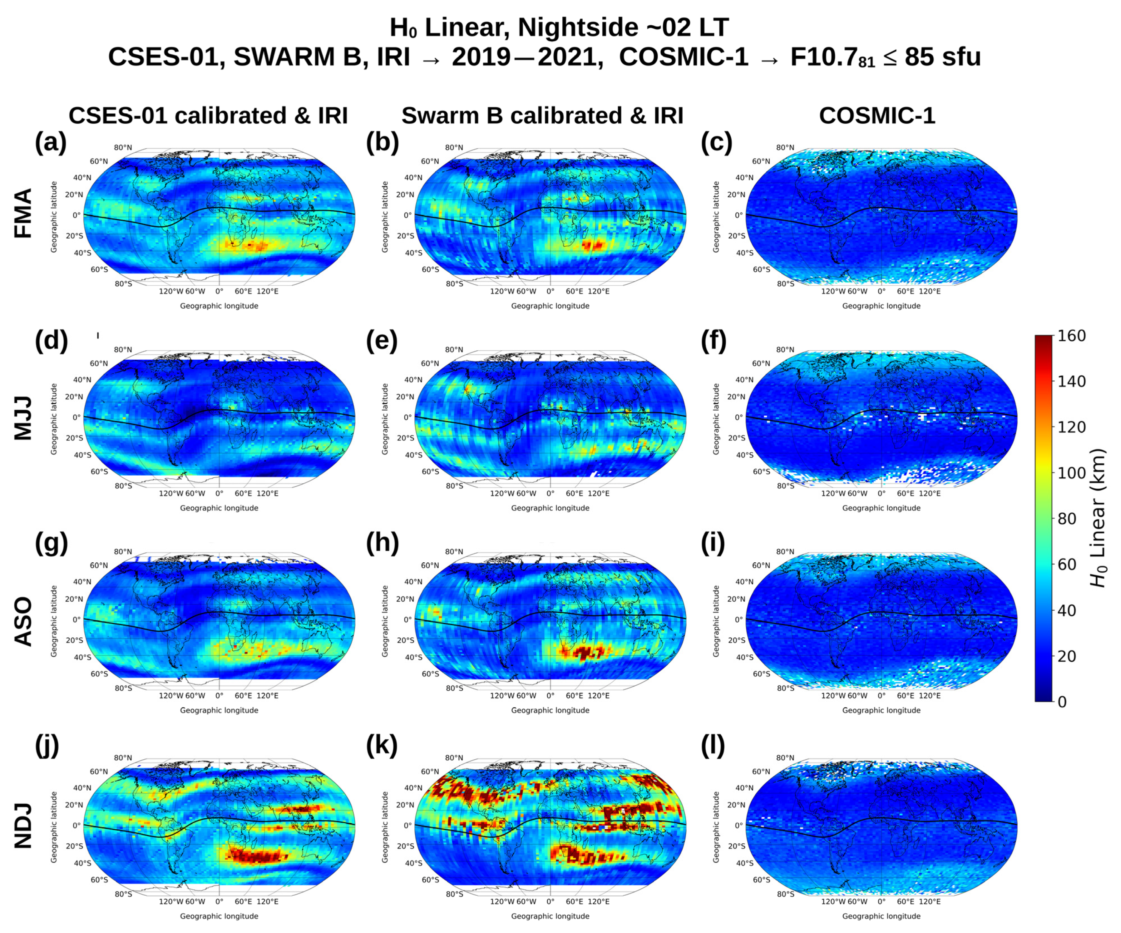
4.1. Topside Effective Scale Height from Calibrated In Situ Ne Observations
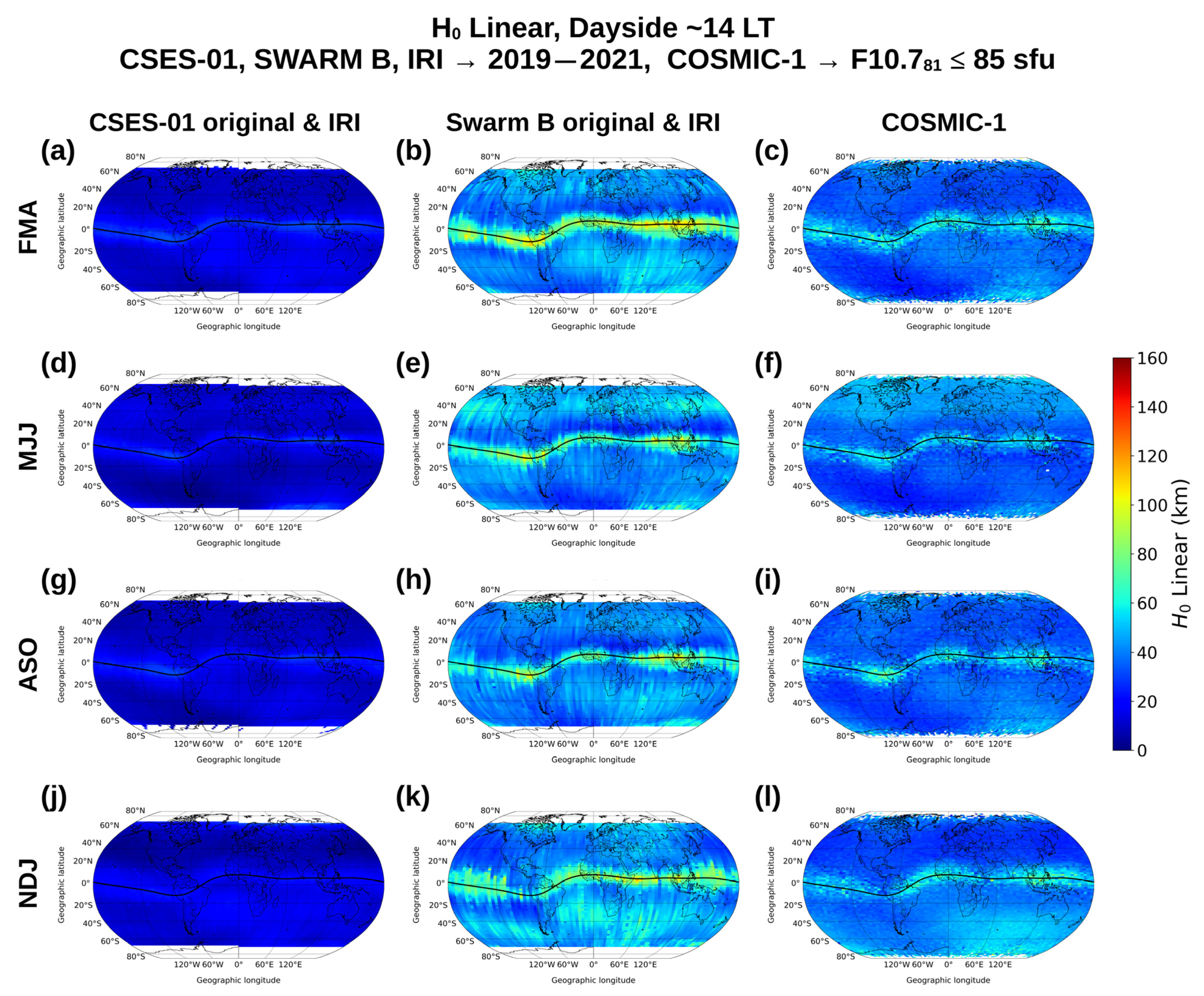
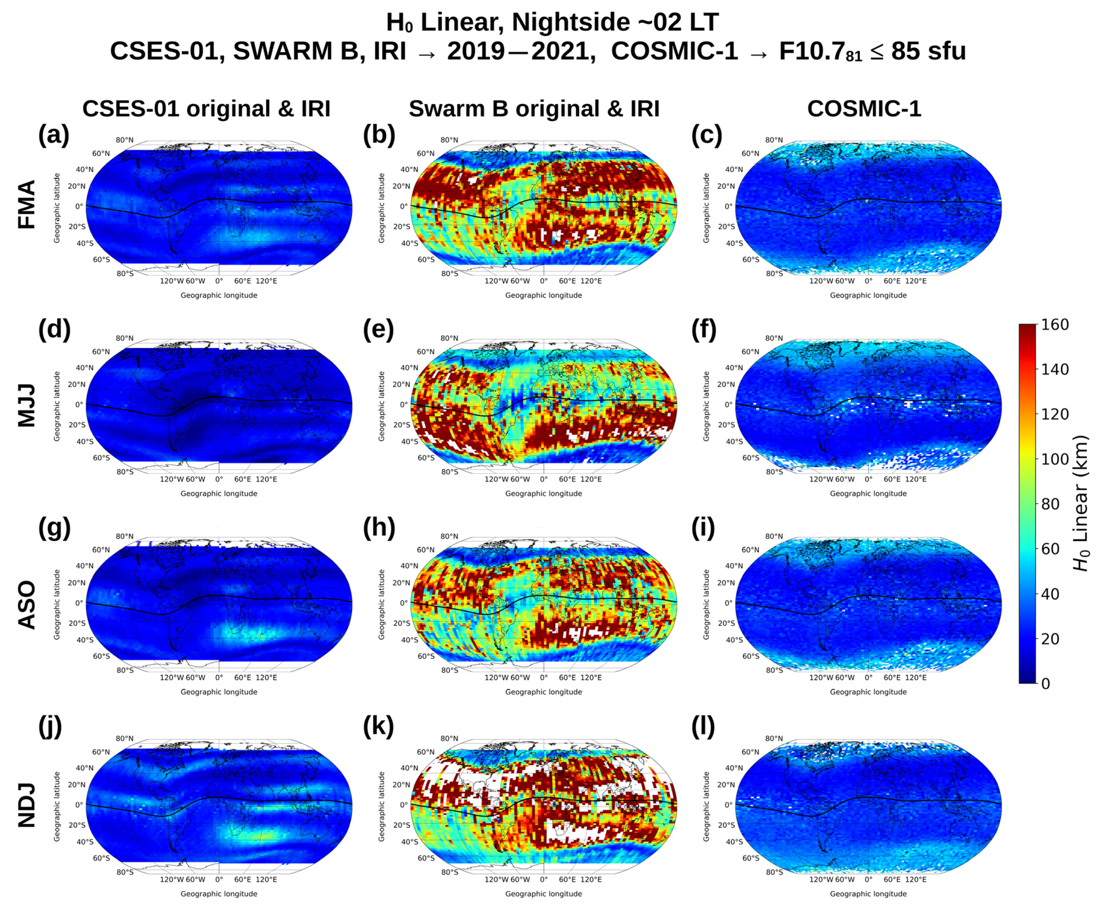
4.2. Topside Effective Scale Height from Non-Calibrated In Situ Ne Observations
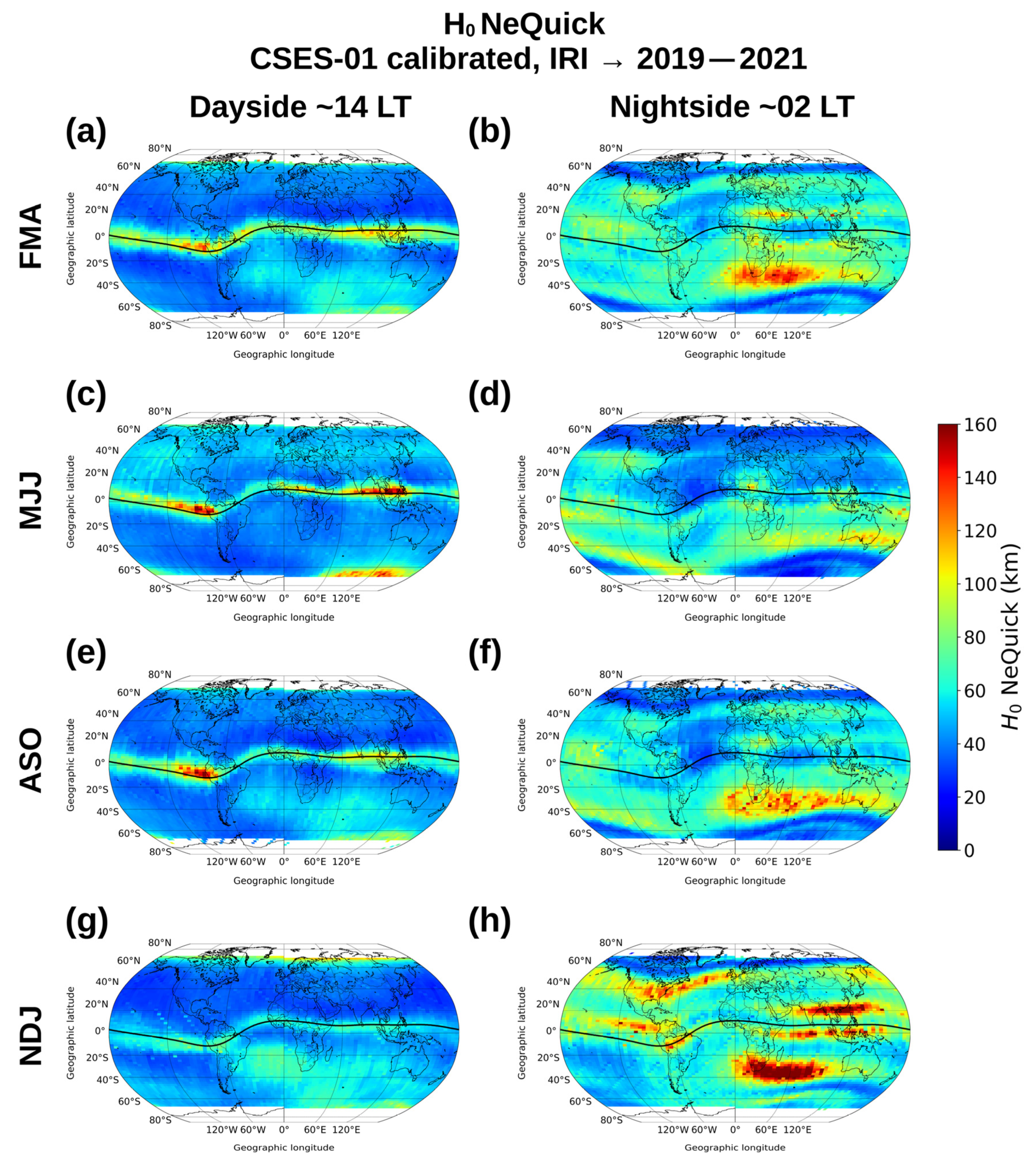
4.3. Topside Effective Scale Height Modeled through the Original NeQuick Formulation
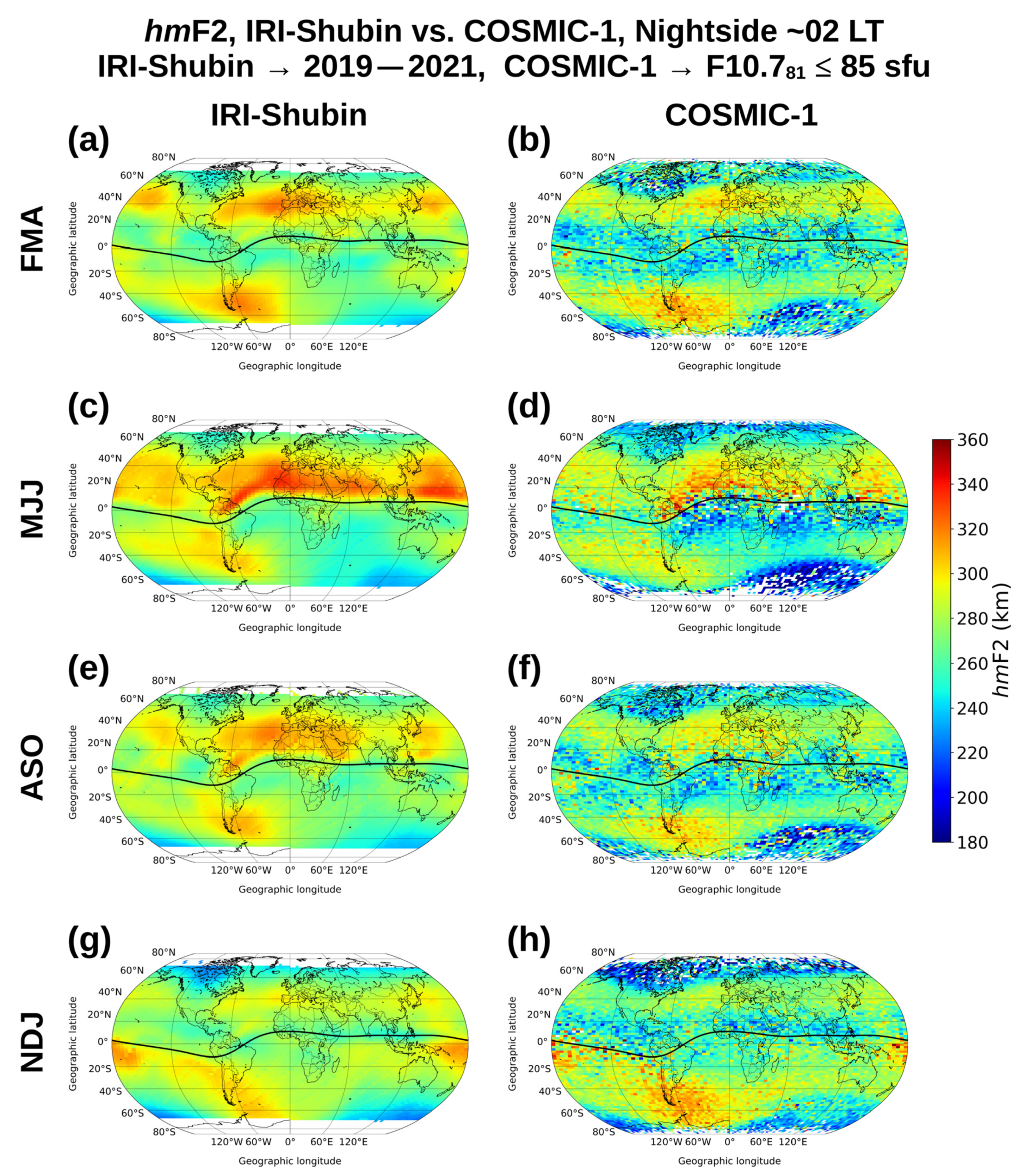
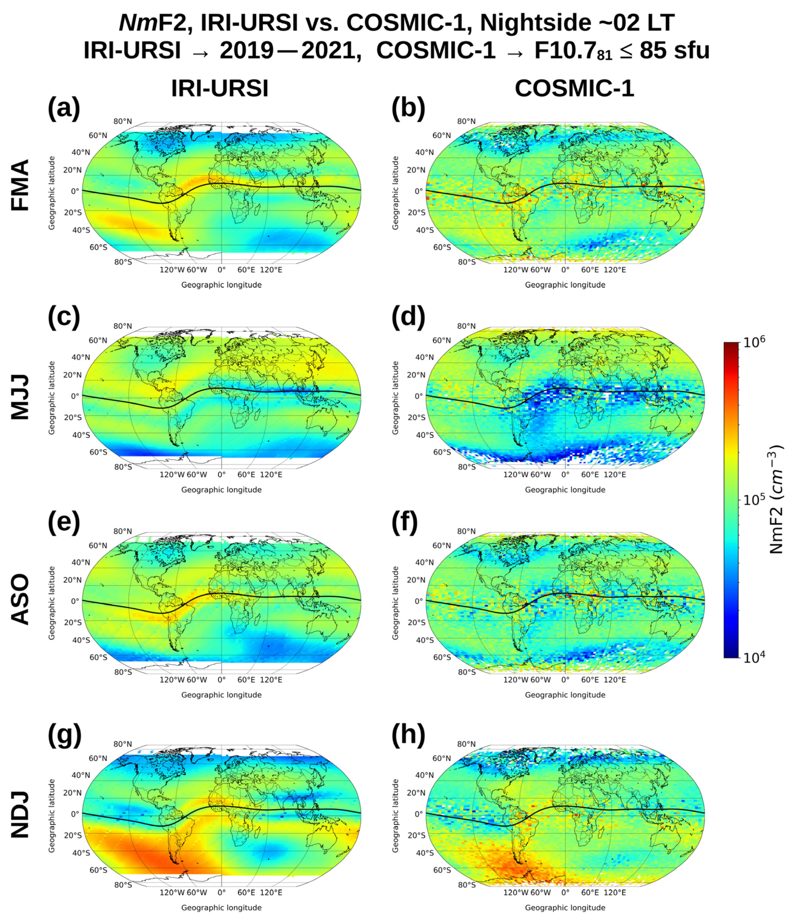
4.4. Comparison between F2-Layer Peak Parameters Modeled by IRI and Measured by COSMIC—1
5. Discussion
6. Conclusions
- For daytime conditions, H0 values modeled using CSES—01 and Swarm B calibrated observations agree with corresponding values obtained directly from COSMIC—1 RO profiles, which is our reference. The geomagnetic equator is where the most relevant differences are present. There, values modeled through both CSES—01 and Swarm B observations are much higher than those obtained through COSMIC—1. Instead, during nighttime, H0 values obtained from both CSES—01 and Swarm B-calibrated observations show large differences compared to those obtained through COSMIC—1. Such differences are spatially localized in several latitudinal belts at both low and mid latitudes, where H0 values obtained from both CSES—01 and Swarm B show values much higher in magnitude than those from COSMIC—1.
- H0 values obtained with non-calibrated CSES—01 and Swarm B observations differ substantially from those obtained with calibrated observations. Except for the Swarm B daytime sector, H0 values from non-calibrated observations show either highly underestimated or overestimated values, which, in most cases, are unphysical. This is an independent piece of evidence that suggest that, for the local times and low solar activity conditions studied in this paper, both CSES—01 and Swarm B LP Ne observations need to be calibrated before being used for ionospheric modeling.
- Most of the H0 mismodeling for nighttime conditions seems to be caused by a sub-optimal spatial representation of the F2-layer peak density made by the IRI model. This issue could be attributed to the IRI spherical harmonics numerical mapping procedure underlying the NmF2 spatial representation, which shows some limitation during nighttime hours. However, the issue is not present for daytime hours. This highlights the importance of an accurate characterization of the F2-layer peak anchor point in topside ionosphere modeling.
Author Contributions
Funding
Data Availability Statement
Acknowledgments
Conflicts of Interest
References
- Rishbeth, H.; Garriott, O. Introduction to Ionospheric Physics; International Geophysics Series; Academic Press: New York, NY, USA, 1969; Volume 14. [Google Scholar]
- Hargreaves, J.K. The Solar-Terrestrial Environment; Cambridge University Press: New York, NY, USA, 1992. [Google Scholar]
- Ratcliffe, J.A. An Introduction to the Ionosphere and Magnetosphere; Cambridge University Press: Cambridge, UK, 1972. [Google Scholar]
- Liu, L.; Le, H.; Wan, W.; Sulzer, M.P.; Lei, J.; Zhang, M.-L. An analysis of the scale heights in the lower topside ionosphere based on the Arecibo incoherent scatter radar measurements. J. Geophys. Res. 2007, 112, A06307. [Google Scholar] [CrossRef]
- Liu, L.; Wan, W.; Zhang, M.-L.; Ning, B.; Zhang, S.-R.; Holt, J.M. Variations of topside ionospheric scale height over Millstone Hill during the 30-day incoherent scatter radar experiment. Ann. Geophys. 2007, 25, 2019–2027. [Google Scholar] [CrossRef]
- Pignalberi, A.; Pezzopane, M.; Nava, B.; Coïsson, P. On the link between the topside ionospheric effective scale height and the plasma ambipolar diffusion, theory and preliminary results. Sci. Rep. 2020, 10, 17541. [Google Scholar] [CrossRef] [PubMed]
- Pignalberi, A.; Pezzopane, M.; Rizzi, R. Modelling the lower part of the topside ionospheric vertical electron density profile over the European region by means of Swarm satellites data and IRI UP method. Space Weather 2018, 16, 304–320. [Google Scholar] [CrossRef]
- Stankov, S.M.; Jakowski, N.; Heise, S.; Muhtarov, P.; Kutiev, I.; and Warnant, R. A new method for reconstruction of the vertical electron density distribution in the upper ionosphere and plasmasphere. J. Geophys. Res. 2003, 108, 1164. [Google Scholar] [CrossRef]
- Verhulst, T.; Stankov, S.M. Evaluation of ionospheric profilers using topside sounding data. Radio Sci. 2014, 49, 181–195. [Google Scholar] [CrossRef]
- Bilitza, D.; Pezzopane, M.; Truhlik, V.; Altadill, D.; Reinisch, B.W.; Pignalberi, A. The International Reference Ionosphere model: A review and description of an ionospheric benchmark. Rev. Geophys. 2022, 60, e2022RG000792. [Google Scholar] [CrossRef]
- Nava, B.; Coïsson, P.; Radicella, S. A new version of the NeQuick ionosphere electron density model. J. Atmos. Sol.-Terr. Phys. 2008, 70, 1856–1862. [Google Scholar] [CrossRef]
- Themens, D.R.; Jayachandran, P.T.; Galkin, I.; Hall, C. The Empirical Canadian High Arctic Ionospheric Model (E-CHAIM): NmF2 and hmF2. J. Geophys. Res. Space Phys. 2017, 122, 9015–9031. [Google Scholar] [CrossRef]
- Hunsucker, R.D. Radio Techniques for Probing the Terrestrial Ionosphere; Springer: Berlin/Heidelberg, Germany, 1991. [Google Scholar] [CrossRef]
- Pignalberi, A.; Pezzopane, M.; Tozzi, R.; De Michelis, P.; Coco, I. Comparison between IRI and preliminary Swarm Langmuir probe measurements during the St. Patrick storm period. Earth Planets Space 2016, 68, 93. [Google Scholar] [CrossRef]
- Shen, X.H.; Zhang, X.M.; Yuan, S.G.; Wang, L.W.; Cao, J.B.; Huang, J.P.; Zhu, X.H.; Picozza, P.; Dai, J.P. The state-of-the-art of the China Seismo-Electromagnetic Satellite mission. Sci. China Technol. Sci. 2018, 61, 634–642. [Google Scholar] [CrossRef]
- Friis-Christensen, E.; Lühr, H.; Knudsen, D.; Haagmans, R. Swarm—An earth observation mission investigating geospace. Adv. Space Res. 2008, 41, 210–216. [Google Scholar] [CrossRef]
- Pignalberi, A.; Pezzopane, M.; Rizzi, R.; Galkin, I. Effective solar indices for ionospheric modelling: A review and a proposal for a real-time regional IRI. Surv. Geophys. 2018, 39, 125–167. [Google Scholar] [CrossRef]
- Pezzopane, M.; Pignalberi, A. The ESA Swarm mission to help ionospheric modelling: A new NeQuick topside formulation for mid-latitude regions. Sci. Rep. 2019, 9, 12253. [Google Scholar] [CrossRef]
- Coïsson, P.; Radicella, S.M.; Leitinger, R.; Nava, B. Topside electron density in IRI and NeQuick: Features and limitations. Adv. Space Res. 2006, 37, 937–942. [Google Scholar] [CrossRef]
- Nava, B.; Radicella, S.M.; Pulinets, S.; Depuev, V. Modelling bottom and topside electron density and TEC with profile data from topside ionograms. Adv. Space Res. 2001, 27, 31–34. [Google Scholar] [CrossRef]
- Olivares-Pulido, G.; Hernández-Pajares, M.; Aragón-Àngel, A.; Garcia-Rigo, A. A linear scale height chapman model supported by GNSS occultation measurements. J. Geophys. Res. Space Phys. 2016, 121, 7932–7940. [Google Scholar] [CrossRef]
- Hernández-Pajares, M.; Garcia-Fernàndez, M.; Rius, A.; Notarpietro, R.; von Engeln, A.; Olivares-Pulido, G.; Aragón-Àngel, À.; García-Rigo, A. Electron density extrapolation above F2 peak by the linear Vary-Chap model supporting new Global Navigation Satellite Systems-LEO occultation missions. J. Geophys. Res. Space Phys. 2017, 122, 9003–9014. [Google Scholar] [CrossRef]
- dos Santos Prol, F.; Themens, D.R.; Hernández-Pajares, M.; de Oliveira Camargo, P.; de Assis Honorato Muella, M.T. Linear vary-chap topside electron density model with topside sounder and radio-occultation data. Surv. Geophys. 2019, 40, 277–293. [Google Scholar] [CrossRef]
- Prol, F.S.; Smirnov, A.G.; Hoque, M.M.; Shprits, Y.Y. Combined model of topside ionosphere and plasmasphere derived from radio-occultation and Van Allen Probes data. Sci. Rep. 2022, 12, 9732. [Google Scholar] [CrossRef]
- Pignalberi, A.; Pezzopane, M.; Themens, D.R.; Haralambous, H.; Nava, B.; Coïsson, P. On the Analytical Description of the Topside Ionosphere by NeQuick: Modelling the Scale Height through COSMIC/FORMOSAT-3 Selected Data. IEEE J. Sel. Top. Appl. Earth Obs. Remote Sens. 2020, 13, 1867–1878. [Google Scholar] [CrossRef]
- Smirnov, A.; Shprits, Y.; Prol, F.; Lühr, H.; Berrendorf, M.; Zhelavskaya, I.; Xiong, C. A novel neural network model of Earth’s topside ionosphere. Sci. Rep. 2023, 13, 1303. [Google Scholar] [CrossRef] [PubMed]
- Anthes, R.; Bernhardt, P.A.; Chen, Y.; Cucurull, L.; Dymond, K.F.; Ector, D.; Healy, S.B.; Ho, S.-P.; Hunt, D.C.; Kuo, Y.-H.; et al. The COSMIC/FORMOSAT-3 mission: Early results. Bull. Amer. Meteorol. Soc. 2008, 89, 313–333. [Google Scholar] [CrossRef]
- Yan, R.; Guan, Y.; Shen, X.; Huang, J.; Zhang, X.; Liu, C.; Liu, D. The Langmuir Probe onboard CSES: Data inversion analysis method and first results. Earth Plan. Phys. 2018, 2, 479–488. [Google Scholar] [CrossRef]
- Liu, C.; Guan, Y.; Zheng, X.; Zhang, A.; Piero, D.; Sun, Y. The technology of space plasma in-situ measurement on the China Seismo-Electromagnetic Satellite. Sci. China Technol. Sci. 2019, 62, 829–838. [Google Scholar] [CrossRef]
- Wang, X.; Cheng, W.; Yang, D.; Liu, D. Preliminary validation of in situ electron density measurements onboard CSES using observations from Swarm Satellites. Adv. Space Res. 2019, 64, 982–994. [Google Scholar] [CrossRef]
- Yan, R.; Zhima, Z.; Xiong, C.; Shen, X.; Huang, J.; Guan, Y.; Zhu, X.; Liu, C. Comparison of electron density and temperature from the CSES satellite with other space-borne and ground-based observations. J. Geophys. Res. Space Phys. 2020, 125, e2019JA027747. [Google Scholar] [CrossRef]
- Liu, J.; Guan, Y.; Zhang, X.; Shen, X. The data comparison of electron density between CSES and DEMETER satellite, Swarm constellation and IRI model. Earth Space Sci. 2021, 8, e2020EA001475. [Google Scholar] [CrossRef]
- Liu, J.; Xu, T.; Ding, Z.; Zhang, X. The Comparison of Electron Density between CSES In Situ and Ground-Based Observations in China. Remote Sens. 2022, 14, 4498. [Google Scholar] [CrossRef]
- Pignalberi, A.; Pezzopane, M.; Coco, I.; Piersanti, M.; Giannattasio, F.; De Michelis, P.; Tozzi, R.; Consolini, G. Inter-Calibration and Statistical Validation of Topside Ionosphere Electron Density Observations Made by CSES—01 Mission. Remote Sens. 2022, 14, 4679. [Google Scholar] [CrossRef]
- Knudsen, D.J.; Burchill, J.K.; Buchert, S.C.; Eriksson, A.I.; Gill, R.; Wahlund, J.-E.; Åhlen, L.; Smith, M.; Moffat, B. Thermal ion imagers and Langmuir probes in the Swarm electric field instruments. J. Geophys. Res. Space Phys. 2017, 122, 2655–2673. [Google Scholar] [CrossRef]
- Lomidze, L.; Knudsen, D.J.; Burchill, J.; Kouznetsov, A.; Buchert, S.C. Calibration and validation of Swarm plasma densities and electron temperatures using ground-based radars and satellite radio occultation measurements. Radio Sci. 2018, 53, 15–36. [Google Scholar] [CrossRef]
- Catapano, F.; Buchert, S.; Qamili, E.; Nilsson, T.; Bouffard, J.; Siemes, C.; Coco, I.; D’Amicis, R.; Tøffner-Clausen, L.; Trenchi, L.; et al. Swarm Langmuir probes’ data quality validation and future improvements. Geosci. Instrum. Method. Data Syst. 2022, 11, 149–162. [Google Scholar] [CrossRef]
- Pakhotin, I.P.; Burchill, J.K.; Förster, M.; Lomidze, L. The swarm Langmuir probe ion drift, density and effective mass (SLIDEM) product. Earth Planets Space 2022, 74, 109. [Google Scholar] [CrossRef]
- Smirnov, A.; Shprits, Y.; Zhelavskaya, I.; Lühr, H.; Xiong, C.; Goss, A.; Prol, F.S.; Schmidt, M.; Hoque, M.; Pedatella, N.; et al. Intercalibration of the plasma density measurements in Earth’s topside ionosphere. J. Geophys. Res. Space Phys. 2021, 126, e2021JA029334. [Google Scholar] [CrossRef]
- Xiong, C.; Jiang, H.; Yan, R.; Lühr, H.; Stolle, C.; Yin, F.; Smirnov, A.; Piersanti, M.; Liu, Y.; Wan, X.; et al. Solar flux influence on the in-situ plasma density at topside ionosphere measured by Swarm satellites. J. Geophys. Res. Space Phys. 2022, 127, e2022JA030275. [Google Scholar] [CrossRef]
- Bilitza, D. IRI the International Standard for the Ionosphere. Adv. Radio Sci. 2018, 16, 1–11. [Google Scholar] [CrossRef]
- Rush, C.M.; Fox, M.; Bilitza, D.; Davies, K.; McNamara, L.; Stewart, F.G.; PoKempner, M. Ionospheric mapping-an update of foF2 coefficients. Telecommun. J. 1989, 56, 179–182. [Google Scholar]
- Shubin, V.N. Global median model of the F2-layer peak height based on ionospheric radio-occultation and ground based digisonde observations. Adv. Space Res. 2015, 56, 916–928. [Google Scholar] [CrossRef]
- Pignalberi, A.; Pietrella, M.; Pezzopane, M. Towards a Real-Time Description of the Ionosphere: A Comparison between International Reference Ionosphere (IRI) and IRI Real-Time Assimilative Mapping (IRTAM) Models. Atmosphere 2021, 12, 1003. [Google Scholar] [CrossRef]
- Haji, G.A.; Romans, L.J. Ionospheric electron density profiles obtained with the global positioning system: Results from the GPS/MET experiment. Radio Sci. 1998, 33, 175–190. [Google Scholar] [CrossRef]
- Schreiner, W.S.; Sokolovskiy, S.V.; Rocken, C.; Hunt, D.C. Analysis and validation of GPS/MET radio occultation data in the ionosphere. Radio Sci. 1999, 34, 949–966. [Google Scholar] [CrossRef]
- Garcia-Fernandez, M.; Hernandez-Pajares, M.; Juan, J.M.; Sanz, J. Improvement of ionospheric electron density estimation with GPSMET occultations using Abel inversion and VTEC information. J. Geophys. Res. Space Phys. 2003, 108, 1338. [Google Scholar] [CrossRef]
- Yue, X.; Schreiner, W.S.; Lei, J.; Sokolovskiy, S.V.; Rocken, C.; Hunt, D.C.; Kuo, Y.H. Error analysis of Abel retrieved electron density profiles from radio occultation measurements. Ann. Geophys. 2010, 28, 217–222. [Google Scholar] [CrossRef]
- UCAR COSMIC Program, 2022; COSMIC—1 Data Products ionPrf. UCAR/NCAR—COSMIC: Boulder, CO, USA, 2022. [CrossRef]
- Tapping, K.F. The 10.7 cm solar radio flux (F10.7). Space Weather 2013, 11, 394–406. [Google Scholar] [CrossRef]
- Pignalberi, A.; Pezzopane, M.; Nava, B. Optimizing the NeQuick topside scale height parameters through COSMIC/FORMOSAT-3 radio occultation data. IEEE Geosc. Rem. Sens. Lett. 2022, 19, 8017005. [Google Scholar] [CrossRef]
- Laundal, K.M.; Richmond, A.D. Magnetic Coordinate Systems. Space Sci. Rev. 2017, 206, 27. [Google Scholar] [CrossRef]
- Themens, D.R.; Jayachandran, P.T.; Bilitza, D.; Erickson, P.J.; Häggström, I.; Lyashenko, M.V.; Reid, B.; Varney, R.H.; Pustovalova, L. Topside electron density representations for middle and high latitudes: A topside parameterization for E-CHAIM based on the NeQuick. J. Geophys. Res. Space Phys. 2018, 123, 1603–1617. [Google Scholar] [CrossRef]
- Mengist, C.K.; Yadav, S.; Kotulak, K.; Bahar, A.; Zhang, S.-R.; Seo, K.-H. Validation of International Reference Ionosphere model (IRI-2016) for F-region peak electron density height (hmF2): Comparison with incoherent scatter radar (ISR) and ionosonde measurements at Millstone Hill. Adv. Space Res. 2020, 65, 2773–2781. [Google Scholar] [CrossRef]
- Huang, H.; Moses, M.; Volk, A.E.; Elezz, O.A.; Kassamba, A.A.; Bilitza, D. Assessment of IRI-2016 hmF2 model options with digisonde, COSMIC observations for low and high solar flux conditions during 23rd solar cycle. Adv. Space Res. 2021, 68, 2093–2103. [Google Scholar] [CrossRef]
- Moses, M.; Bilitza, D.; Kumar Panda, S.; Ochonugor, B.J. Assessment of IRI-2016 hmF2 model predictions with COSMIC observations over the African region. Adv. Space Res. 2021, 68, 2115–2123. [Google Scholar] [CrossRef]
- Jones, W.B.; Gallet, R.M. Representation of diurnal and geographical variations of ionospheric data by numerical methods. J. Res. Natl. Bur. Stand. 1962, 66, 129–147. [Google Scholar] [CrossRef]
- Jones, W.B.; Gallet, R.M. Representation of diurnal and geographic variations of ionospheric data by numerical methods, II. Control of instability. ITU Telecommun. J. 1965, 32, 18–28. [Google Scholar]
- Jones, W.B.; Graham, R.P.; Leftin, M. Advances in ionospheric mapping by numerical methods. In ESSA Technical Report ERL 107-ITS75; U.S. Department of Commerce: Washington, DC, USA, 1969. [Google Scholar]
- Rawer, K. Propagation of decameter waves (HF band). In Meteorological and Astronomical Influences on Radio Wave Propagation; Landmark, B., Ed.; Academic Press: Cambridge, MA, USA, 1963; pp. 221–250. [Google Scholar]
- Li, Q.; Liu, L.; He, M.; Huang, H.; Zhong, J.; Yang, N.; Zhang, M.-L.; Jiang, J.; Chen, Y.; Le, H.; et al. A global empirical model of electron density profile in the F region ionosphere basing on COSMIC measurements. Space Weather 2021, 19, e2020SW002642. [Google Scholar] [CrossRef]
- Pignalberi, A.; Nava, B.; Pietrella, M.; Cesaroni, C.; Pezzopane, M. Midlatitude climatology of the ionospheric equivalent slab thickness over two solar cycles. J. Geod. 2021, 95, 124. [Google Scholar] [CrossRef]
- Pignalberi, A.; Pietrella, M.; Pezzopane, M.; Nava, B.; Cesaroni, C. The Ionospheric Equivalent Slab Thickness: A Review Supported by a Global Climatological Study over Two Solar Cycles. Space Sci. Rev. 2022, 218, 37. [Google Scholar] [CrossRef]
- Titheridge, J.E. The slab thickness of the mid-latitude ionosphere. Planet. Space Sci. 1973, 21, 1775–1793. [Google Scholar] [CrossRef]
- Jakowski, N.; Hoque, M.; Mielich, J.; Hall, C. Equivalent slab thickness of the ionosphere over Europe as an indicator of long-term temperature changes in the thermosphere. J. Atmos. Sol.-Terr. Phys. 2017, 163, 91–102. [Google Scholar] [CrossRef]


Disclaimer/Publisher’s Note: The statements, opinions and data contained in all publications are solely those of the individual author(s) and contributor(s) and not of MDPI and/or the editor(s). MDPI and/or the editor(s) disclaim responsibility for any injury to people or property resulting from any ideas, methods, instructions or products referred to in the content. |
© 2023 by the authors. Licensee MDPI, Basel, Switzerland. This article is an open access article distributed under the terms and conditions of the Creative Commons Attribution (CC BY) license (https://creativecommons.org/licenses/by/4.0/).
Share and Cite
Pignalberi, A.; Pezzopane, M.; Alberti, T.; Coco, I.; Consolini, G.; D’Angelo, G.; De Michelis, P.; Giannattasio, F.; Nava, B.; Piersanti, M.; et al. Modeling the Topside Ionosphere Effective Scale Height through In Situ Electron Density Observations by Low-Earth-Orbit Satellites. Universe 2023, 9, 280. https://doi.org/10.3390/universe9060280
Pignalberi A, Pezzopane M, Alberti T, Coco I, Consolini G, D’Angelo G, De Michelis P, Giannattasio F, Nava B, Piersanti M, et al. Modeling the Topside Ionosphere Effective Scale Height through In Situ Electron Density Observations by Low-Earth-Orbit Satellites. Universe. 2023; 9(6):280. https://doi.org/10.3390/universe9060280
Chicago/Turabian StylePignalberi, Alessio, Michael Pezzopane, Tommaso Alberti, Igino Coco, Giuseppe Consolini, Giulia D’Angelo, Paola De Michelis, Fabio Giannattasio, Bruno Nava, Mirko Piersanti, and et al. 2023. "Modeling the Topside Ionosphere Effective Scale Height through In Situ Electron Density Observations by Low-Earth-Orbit Satellites" Universe 9, no. 6: 280. https://doi.org/10.3390/universe9060280
APA StylePignalberi, A., Pezzopane, M., Alberti, T., Coco, I., Consolini, G., D’Angelo, G., De Michelis, P., Giannattasio, F., Nava, B., Piersanti, M., & Tozzi, R. (2023). Modeling the Topside Ionosphere Effective Scale Height through In Situ Electron Density Observations by Low-Earth-Orbit Satellites. Universe, 9(6), 280. https://doi.org/10.3390/universe9060280