The Finsler Spacetime Condition for (α,β)-Metrics and Their Isometries

Abstract

For the general class of pseudo-Finsler spaces with $(\alpha ,\beta )$-metrics, we establish necessary and sufficient conditions such that these admit a Finsler spacetime structure. This means that the fundamental tensor has a Lorentzian signature on a conic subbundle of the tangent bundle and thus the existence of a cone of future-pointing time-like vectors is ensured. The identified $(\alpha ,\beta )$-Finsler spacetimes are candidates for applications in gravitational physics. Moreover, we completely determine the relation between the isometries of an $(\alpha ,\beta )$-metric and the isometries of the underlying pseudo-Riemannian metric a; in particular, we list all $(\alpha ,\beta )$-metrics which admit isometries that are not isometries of a.

1. Introduction

Finsler geometry, which is the geometry of a manifold described by a general geometric length measure for curves, has numerous applications in physics [1]. In the context of gravitational physics, it is the perfect mathematical framework to describe the gravitational field of a kinetic gas [2,3], it models the propagation of particles subject to deformed/doubly special relativity symmetries employed in quantum gravity phenomenology [4,5,6], and it emerges naturally in the context of theories based on broken/deformed Lorentz invariance, such as the standard model extension (SME) [7,8,9] or very special relativity (VSR) [10].

In general, Finsler geometry allows for a huge variety of structures, which are much more varied than those of pseudo-Riemannian structures on manifolds. Therefore, it is important to classify Finsler geometries in order to identify the best models for specific applications.

Among all Finsler structures, the class of $(\alpha ,\beta )$-metrics, obtained by constructing a geometric length measure for curves from a (pseudo)-Riemannian metric a and a 1-form b, are the easiest to construct and the most used in practice. Notorious examples include Bogoslovsky–Kropina (or m-Kropina) metrics, which represent the framework for VSR and its generalization, very general relativity (VGR) [10,11,12,13,14]—also used for dark energy models [15]—and Randers metrics, used, for instance, in the description of the propagation of light in stationary spacetimes [16,17,18,19], for the motion of an electrically charged particle in an electromagnetic field, in the study of Finsler gravitational waves [20,21], as an extended background for field theories [22] and black holes [23], or in Zermelo’s navigation problem [16,24].

All the above-mentioned applications require Finsler metrics of Lorentzian signature. While there exists a rich literature on positive definite Finsler metrics (and in particular, on $(\alpha ,\beta )$-ones [25,26,27,28,29,30]), Lorentzian Finsler geometry is by far least understood and investigated [31]. In this paper, we study for the first time in full generality two questions about Lorentzian $(\alpha ,\beta )$-Finsler structures, which have been only partially tackled in the literature (mostly only for very particular cases):

1.

The necessary and sufficient conditions for an $(\alpha ,\beta )$-metric to define a Finsler spacetime structure;

2.

Determining the isometries of general $(\alpha ,\beta )$-metrics.

Regarding point 1. above, the very definition of a Finsler spacetime is actually still a matter of debate [32,33,34,35,36,37,38,39,40,41]. Yet, in recent years, though the various definitions may differ in their minute details, they all converge to the following understanding: at each point of a Finslerian spacetime, there should exist a convex cone with null boundary—interpreted as the cone of future-pointing time-like vectors—on which the Finsler metric tensor must be well defined, smooth (maybe with the exception of one singular direction [38]), and with Lorentzian signature.

Starting from this understanding, we determine the conditions for a general $(\alpha ,\beta )$-metric, with a completely arbitrary 1-form, to be smooth and to have Lorentzian signature inside such a cone. Furthermore, we present concrete examples that are interesting for applications such as Randers and Bogoslovsky–Kropina metrics (extending previous studies [12,42] for the case of non-space-like 1-forms) as well as generalized m-Kropina and exponential metrics.

For the second problem, isometries of $(\alpha ,\beta )$-metrics, to the best of our knowledge, the only cases when these were known are Bogoslovsky–Kropina deformations of Minkowski metrics [28,43], as well as Randers and Kropina metrics [27]. Here, we determine infinitesimal isometries of general $(\alpha ,\beta )$-metrics.

The structure of this paper is as follows. Section 2 reviews the necessary notions of Finsler spacetimes for our later construction. Section 3 consists of the investigation of the conditions for an $(\alpha ,\beta )$-metric to define a spacetime structure, and presents our main theorem, Theorem 1. A complete classification, using simple conditions, is then given for the most used classes in Section 4. In Section 5, we determine the infinitesimal isometries of general $(\alpha ,\beta )$-metrics. Section 6 briefly presents our conclusions. In Appendix A, we display the proof of our formula for the determinant of the fundamental tensor of a general $(\alpha ,\beta )$-metric and of its inverse.

2. Preliminaries

We begin by recalling the concept of a Finsler spacetime in this section.

There are numerous attempts to find a suitable definition of a Finsler spacetime, i.e., of pseudo-Finsler geometry with a Finsler metric of Lorentzian signature, where among the first are those of Beem [40] and Asanov [41]. However, it quickly turned out that these definitions given are too restrictive to cover numerous interesting physical examples, such as m-th root metrics, Randers metrics, or m-Kropina metrics. Since then, several definitions of Finsler spacetimes have been developed [32,33,34,35,36,37,38,39], all agreeing that the Finsler metric tensor should be of Lorentzian signature on some (conic) subset of the tangent bundle, but differing in the precise details of where it must be smooth or only continuous. The origin of these fine differences lies in the various applications and examples on which the authors focused when formulating their definitions; thorough discussions of the differences between the distinct approaches to indefinite Finsler spacetime geometry can be found, e.g., in [34,39].

In the following, we will use the notion of Finsler spacetime as defined by two of us in [39], as it is the most permissive one which still allows for well-defined curvature-related quantities on the entire future-pointing time-like domain. Yet, as we will point out below, our approach can be applied with a minimal modification to the (even more permissive) definition by Caponio and co-workers [37,38].

Prior to introducing the notion of Finsler spacetime, we briefly introduce the manifolds we are working on and the preliminary notions of conic subbundle and pseudo-Finsler structure.

For the whole article, let M be a four-dimensional, connected, orientable, smooth manifold, let $(TM,\pi ,M)$ be its tangent bundle, and $\stackrel{\circ }{TM}=TM\backslash \left\{0\right\}$ be the tangent bundle without its zero section. We will denote the coordinates of a point $x\in U\subset M$ in a local chart $\left(U,\phi \right)$ by ${\left(x^i\right)}_{i=\overline{0,3}},$ and the naturally induced local coordinates of points $(x,\dot{x})\in {\pi }^{-1}\left(U\right)$ by $(x^i,{\dot{x}}^i)$. Commas ${}_{,i}$ denote partial differentiation with respect to the coordinates $x^i$ and dots ${}_{·i}$ denote partial differentiation of coordinates ${\dot{x}}^i.$ Furthermore, whenever there is no risk of confusion, we will omit for simplicity the indices of the coordinates.

A conic subbundle of $TM$ is a non-empty open submanifold $\mathcal{Q}\subset \stackrel{\circ }{TM}$, which projects by $\pi$ on the entire manifold, i.e., $\pi \left(\mathcal{Q}\right)=M$, and possesses the so-called conic property:

$$(x,\dot{x})\in \mathcal{Q}\Rightarrow (x,\lambda \dot{x})\in \mathcal{Q},\forall \lambda >0.$$

Furthermore, a pseudo-Finsler structure on M, see [44], is a smooth function $L:\mathcal{A}\to \mathbb{R}$ defined on a conic subbundle $\mathcal{A}\subset \stackrel{\circ }{TM}$, obeying the following conditions:

1.

Positive two-homogeneity: $L(x,\alpha \dot{x})={\alpha }^{2}L(x,\dot{x}),\forall \alpha >0,$ $\forall (x,\dot{x})\in \mathcal{A}.$

2.

At any $\left(x,\dot{x}\right)\in \mathcal{A}$ and in one (and then, in any) local chart around $(x,\dot{x}),$ the Hessian:

$$g_{ij}={\displaystyle \frac{1}{2}}{\displaystyle \frac{{\partial }^{2}L}{\partial {\dot{x}}^i\partial {\dot{x}}^j}}={\displaystyle \frac{1}{2}}{L}_{·i·j}$$

(1)

is nondegenerate.

We note that, in general, the functions $g_{ij}=g_{ij}(x,\dot{x})$ have a nontrivial $\dot{x}$-dependence; more precisely, they define a mapping

$$g:\mathcal{A}\to T_2^{0}M,\left(x,\dot{x}\right)\mapsto g_{(x,\dot{x})}=g_{ij}(x,\dot{x})d{x}^i\otimes d{x}^j,$$

(2)

called the Finslerian metric tensor. This is generally not a tensor field on M (as it depends on vectors $\dot{x}\in T_{x}M$), but it plays a largely similar role to the one of the metric tensor in pseudo-Riemannian geometry. The particular case when $g=g_{\left(x\right)}$ only (that is, $L(x,\dot{x})=a_{ij}\left(x\right){\dot{x}}^i{\dot{x}}^j$ is quadratic in $\dot{x}$) corresponds to pseudo-Riemannian geometry, see, for example, [45].

Definition 1

(Finsler spacetime, following [39]). A Finsler spacetime $\left(M,L\right)$, is a four-dimensional manifold M with a pseudo-Finsler structure $L:\mathcal{A}\to \mathbb{R}$ (where M is connected and orientable), obeying the additional third condition:

3.

There exists a connected conic subbundle $\mathcal{T}\subset \mathcal{A}$ with connected fibers ${\mathcal{T}}_x=\mathcal{T}\cap T_{x}M,$ $x\in M,$ such that on each ${\mathcal{T}}_x:$$L>0,$g has a Lorentzian signature $(+,-,-,-)$ and L can be continuously extended as 0 to the boundary $\partial {\mathcal{T}}_x.$

Physically, the Finsler spacetime function L is interpreted as the interval $d{s}^2=L(x,dx)$.

• On a Finsler spacetime, there exists the following important subsets of $TM$:

• The conic subbundle $\mathcal{A}$ where L is defined, smooth, and contains nondegenerate Hessians is called the set of admissible vectors; we will typically understand $\mathcal{A}$ as the maximal subset of $\stackrel{\circ }{TM}$ with these properties.
• The conic subbundle $\mathcal{T},$ where the signature of g and the sign of L agree, will be interpreted as the set of future-pointing time-like vectors.

Note. From the above definition, it follows that all the fibers ${\mathcal{T}}_x$ of $\mathcal{T}$ are actually convex cones, see [39].

The definition in [34] can be recovered by setting $\mathcal{A}=\mathcal{T}$ and imposing that L extends smoothly to the boundary $\partial \mathcal{T}$, whereas the definition in [37,38] can be recovered by allowing L to be of class ${\mathcal{C}}^1$ only along one direction in each cone ${\mathcal{T}}_x$.

In a Finsler spacetime, the arc length of a curve $\gamma :[a,b]\to M,t\mapsto \gamma \left(t\right):$

$$l_{\gamma }=\stackrel{b}{\underset{a}{\int }}\sqrt{\left|L\left(\gamma \left(t\right),\dot{\gamma }\left(t\right)\right)\right|}dt$$

is well defined (independent of the parametrization), by virtue of the two-homogeneity of $L.$ Moreover, for future-pointing time-like curves (defined by the fact that $\dot{\gamma }\left(t\right)=\frac{d\gamma \left(t\right)}{dt}$ belongs to the cone ${\mathcal{T}}_{\gamma \left(t\right)}$ for all t—interpreted as worldlines of massive particles), it gives the proper time along the respective worldline.

Having clarified our notion of Finsler spacetimes, we can proceed and present general conditions for $(\alpha ,\beta )$-Finsler metrics, so that they indeed define Finsler spacetimes.

3. Spacetime Conditions for $\left(\mathbf{\alpha },\mathbf{\beta }\right)$-Metrics

Finsler metrics of $(\alpha ,\beta )$-type can nicely be classified and studied due to their fairly simple building blocks, which are a pseudo-Riemannian metric a and a 1-form b on M.

More precisely, consider a Lorentzian metric $a=a_{ij}d{x}^i\otimes d{x}^j$ (we use the signature convention $\left(+,-,-,-\right)$) and a 1-form $b=b_{i}d{x}^i$ on M. Let us denote, in any local chart:

$$B=b\left(\dot{x}\right)=b_i{\dot{x}}^i,A\left(x,\dot{x}\right)=a_x\left(\dot{x},\dot{x}\right)=a_{ij}{\dot{x}}^i{\dot{x}}^j;$$

(3)

in comparison to the usual notations $\alpha ,\beta$ in the literature on positive definite Finsler spaces, this is:

$$\begin{array}{c}\hfill \alpha =\sqrt{\left|A\right|},\beta =B.\end{array}$$

(4)

Throughout the paper, for simplicity, we will also refer to the Lorentzian metric a as A.

An $\left(\alpha ,\beta \right)$-metric on M is, by definition, a pseudo-Finsler structure $L:\mathcal{A}\to \mathbb{R}$ (where $\mathcal{A}\subset \stackrel{\circ }{TM}$ is a conic subbundle) of the form:

$$L=A\mathsf{\Psi }\left(s\right),s={\displaystyle \frac{B^2}{A}},$$

(5)

where $\mathsf{\Psi }=\mathsf{\Psi }\left(s\right)$ is smooth on the set $s\left(\mathcal{A}\right)$ of values $s\in \mathbb{R}$ corresponding to vectors in $\mathcal{A}$.

The metric tensor components $g_{ij}=g_{ij}(x,\dot{x})$ are easily found as:

$$g_{ij}=a_{ij}(\mathsf{\Psi }-s{\mathsf{\Psi }}^{\prime })+{\mathsf{\Psi }}^{\prime }{b}_i{b}_j+{\displaystyle \frac{1}{2}}{A}^2{\mathsf{\Psi }}^{″}{s}_{·i}{s}_{·j},$$

(6)

with inverse (A10) given in Appendix A, see also [13].

In the following, we will investigate the conditions such that functions L as in (5) define a Finsler spacetime structure on $M.$ In other words, we will investigate the existence of a conic subbundle $\mathcal{T}\subset \mathcal{A}$ satisfying the requirement of Definition 1. With this aim, let us make the following assumption:

Assumption 1.

At each $x\in M,$ the cone ${\mathcal{T}}_x$ of $L$ and the future-pointing time-like cone ${\mathcal{T}}_x^a$ of the metric a have a non-empty intersection.

In other words, subluminal speeds of particles, as measured by a Finslerian observer, are not all superluminal from the point of view of an observer using a (pseudo-)Riemannian arc length.

Fix, in the following, an arbitrary point $x\in M$ and an arbitrary local chart with local coordinates $\left(x^i,{\dot{x}}^i\right)$ in a neighborhood of ${\pi }^{-1}\left(x\right).$ In the following, we will omit the point x from the writing of $\left(x,\dot{x}\right)$-dependent quantities; that is, we will write simply $L=L\left(\dot{x}\right),$ $A=A\left(\dot{x}\right),$ $g_{\dot{x}}=g_{(x,\dot{x})}$, etc.

We denote by $〈,〉$ the scalar product with respect to $a_x$, that is:

$$A:=〈\dot{x},\dot{x}〉,〈b,b〉=a^{ij}{b}_i{b}_j=a_{ij}{\tilde{b}}^i{\tilde{b}}^j,〈\tilde{b},\dot{x}〉=b\left(\dot{x}\right)=B,$$

(7)

where tildes are used to indicate the raising/lowering of indices by a, e.g., ${\tilde{b}}^i=a^{ij}{b}_j$ (in contrast, we will not use tildes when raising/lowering indices with $g;$ that is, $b^i=g^{ij}{b}_j$, etc.).

Remark 1.

1.

Using the above assumption ${\mathcal{T}}_x\cap {\mathcal{T}}_x^a\ne ⌀$ and $L_{|{\mathcal{T}}_x}>0$, it follows that:

$$\forall \dot{x}\in {\mathcal{T}}_x:A>0,\mathsf{\Psi }>0;$$

(8)

in particular, ${\mathcal{T}}_x$ must be completely contained in the future-pointing cone of a.

Indeed, according to the mentioned assumption, for any $x\in M$, there exists at least one vector y in the intersection ${\mathcal{T}}_x\cap {\mathcal{T}}_x^a$ which thus must satisfy $A\left(y\right)>0,\mathsf{\Psi }\left(y\right)>0$. As both a A and Ψ are assumed to be smooth (and hence, continuous) on ${\mathcal{T}}_x$, in order to change sign, they should pass through 0. But the vanishing of either A or Ψ entails $L=0$, which is in contradiction with the positiveness axiom for L inside $\mathcal{T}$; therefore, (8) must hold throughout ${\mathcal{T}}_x$.

2.

On the boundary $\partial {\mathcal{T}}_x,$ L can be continuously prolonged as to satisfy:

$$A=0or\mathsf{\Psi }=0.$$

(9)

Lemma 1 (The domain of$s$).

In any $\left(\alpha ,\beta \right)$-metric Finsler spacetime, the set of values s such that $s\left(\dot{x}\right)\in {\mathcal{T}}_x$ is an interval

$$I\subset [s_0,\infty ),s_0:=max\{〈b,b〉,0\}.$$

(10)

Proof. 

Let us first show that the set $I=\left\{s\left(\dot{x}\right)|\dot{x}\in {\mathcal{T}}_x\right\}$ is contained in $[s_0,\infty )$, that is:

$$s\left(\dot{x}\right)\ge s_0,\forall \dot{x}\in {\mathcal{T}}_x.$$

If b is a-time-like, i.e., $〈b,b〉>0,$ then, taking into account that $\dot{x}$ is by definition also a-time-like, the reverse Cauchy–Schwarz inequality tells us that: $〈b,b〉〈\dot{x},\dot{x}〉\le {〈b,\dot{x}〉}^2,$ which, using (7), is nothing but:

$$〈b,b〉A\le B^2;$$

that is,

$$s\ge 〈b,b〉\Rightarrow s\ge max\{〈b,b〉,0\}=s_0.$$

In the case when $〈b,b〉\le 0,$ the statement is trivially satisfied, as $s={\displaystyle \frac{B^2}{A}}$ is the ratio of two quantities that are non-negative on ${\mathcal{T}}_x$, and hence $s\ge 0=s_0$.

Furthermore, since on ${\mathcal{T}}_x,$ $A\ne 0,$ the rational function $s=s\left(\dot{x}\right):{\mathcal{T}}_x\to \mathbb{R}$ is continuous; using the connectedness axiom for ${\mathcal{T}}_x,$ it follows that $I=s\left({\mathcal{T}}_x\right)\subset \mathbb{R}$ must also be connected; namely, it is an interval. □

In Figure 1 below, we represent various relative positions of the future-pointing cone ${\mathcal{T}}_x^a$ of A (in orange) and the conic set $\mathsf{\Psi }>0$ (in blue). It is important to note that the cone ${\mathcal{T}}_x$ is always the intersection of these two sets.

Remark 2 (sharpness (or non-sharpness) of the bounds for $s$). To precisely establish the interval I, we first need the critical points of the function $s=s\left(\dot{x}\right)$. These turn out to be situated:

• In the plane $B=0$; in this case, the corresponding critical value is $s=0$.
• On the ray directed by $\dot{x}=\tilde{b}$ emanating from the origin; this yields the critical value $s=〈b,b〉$.

The above statement is justified as follows. Differentiating the expression $s=\frac{B^2}{A}$, we find that the condition ${\dot{\partial }}_{i}s=0$ is equivalent to:

$$B(b_{i}A-B{a}_{ij}{\dot{x}}^j)=0.$$

(11)

The vanishing of the first factor means precisely $B=0$, whereas the second one gives, after raising indices with the help of $a^{jk}$, that $\dot{x}$ is proportional to $\tilde{b}$.

• Taking into account the above Lemma, we note that the corresponding critical values are—if attained inside ${\mathcal{T}}_x$—minimal values for s. This way, we find:

1.

The lower bound $s=s_0$ is attained for $\dot{x}\in {\mathcal{T}}_x$ in two situations:

i.

When $b\in {\mathcal{T}}_x$ is L-time-like (which implies that, in particular, it is also a-time-like, meaning that $〈b,b〉>0$) and $\dot{x}$ is collinear to $\tilde{b}$;

ii.

When the critical hyperplane $B=0$ for s intersects ${\mathcal{T}}_x$ (a necessary condition for this is that b is a-space-like).

2.

For the upper bound, we have two possibilities:

i.

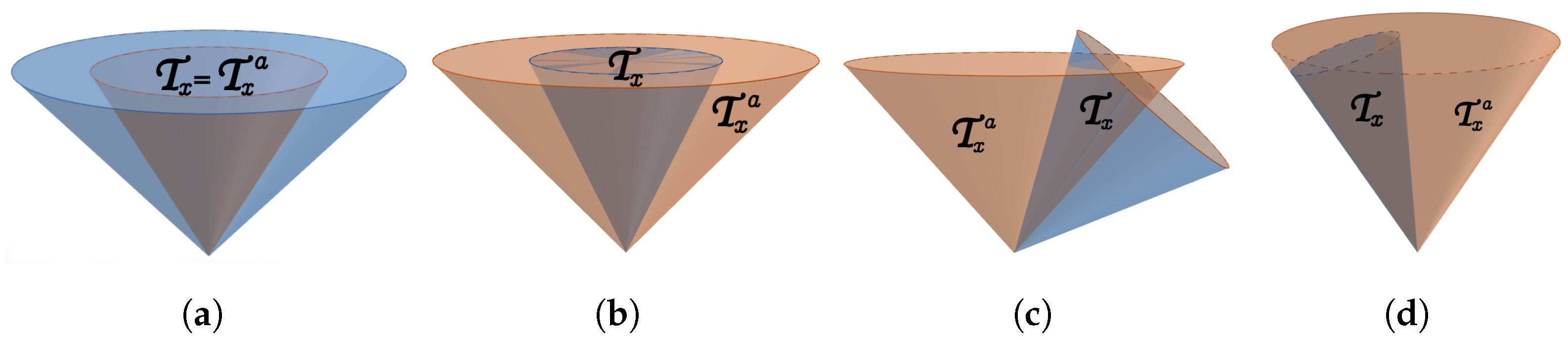
If the boundary $\partial {\mathcal{T}}_x$ contains points where $A=0,B\ne 0,$ (as in Figure 1a,c,d), then, approaching these points, we will have $s\to \infty ;$ therefore, in this case, $s\in [s_0,\infty ),$ where the upper bound is sharp.

ii.

If A does not vanish anywhere on $\partial {\mathcal{T}}_x$ (situation (b) in Figure 1, when $\partial {\mathcal{T}}_x$ consists only of points where $\mathsf{\Psi }=0,$ $A>0$), then—since obviously we cannot have $A=0$inside${\mathcal{T}}_x$ either—it follows that s has a finite supremum on ${\mathcal{T}}_x$, in other words, we can safely write $s\in [s_0,s_1)$ for some finite value $s_1>0.$

Having determined the domain of s, the next step for determining the precise conditions relating $\mathsf{\Psi }$ and $〈b,b〉$ such that L defines a spacetime structure is to find the sign of the coefficient $\mathsf{\Psi }-s{\mathsf{\Psi }}^{\prime }$ in (6).

Lemma 2.

In any $\left(\alpha ,\beta \right)$-metric Finsler spacetime and at any $\dot{x}\in {\mathcal{T}}_x,$ it holds that:

$$\mathsf{\Psi }-s{\mathsf{\Psi }}^{\prime }>0.$$

Proof. 

Let $I=s\left({\mathcal{T}}_x\right)\subset [s_0,\infty )$ be the interval defined above. We will proceed in three steps:

Step 1.

There exists at least one $\dot{x}$ on the boundary $\partial {\mathcal{T}}_x$ such that $B\left(\dot{x}\right)\ne 0:$

Pick an arbitrary $v\in \partial {\mathcal{T}}_x.$ If v does not belong to the hyperplane $H:=\left\{v\in T_{x}M|B\left(v\right)=0\right\}$, then the statement is proven with $\dot{x}=v.$

Hence, in the following, let us assume that $v\in \partial {\mathcal{T}}_x\cap H.$

The cone ${\mathcal{T}}_x$ is, by definition, open (in the topology of $T_{x}M\simeq {\mathbb{R}}^4$); therefore, it cannot be entirely contained in the hyperplane $H.$ This way, there exists $u\in {\mathcal{T}}_x$ such that $B\left(u\right)\ne 0$. We will show that, going along the line:

$$\ell :=\{u-\lambda v|\lambda \in \mathbb{R}\}$$

we must encounter a boundary point which is not in $H:$

-

We first note that ℓ has no common points with $H.$ Indeed, for any $\lambda \in \mathbb{R},$ we have $B(u-\lambda v)=B\left(u\right)-\lambda B\left(v\right)=B\left(u\right)\ne 0.$

-

Second, $\ell \cap {\overline{\mathcal{T}}}_x$ is a non-empty, connected set. Indeed, ℓ contains an interior point of ${\mathcal{T}}_x,$ which is u. Moreover, since ${\mathcal{T}}_x$ is convex, this means that its closure—which is also necessarily convex—must intersect ℓ by a segment, a half-line, or the whole ℓ. In any case, $\ell \cap {\overline{\mathcal{T}}}_x$ is connected.

-

Third, we show that the set ${\overline{\mathcal{T}}}_x\cap \ell$ intersects the cone ${\mathcal{T}}_x^a:A=0.$ To this aim, let us build the function $f:\mathbb{R}\to \mathbb{R},$

$$f\left(\lambda \right):=A\left(u-\lambda v\right)=〈u,u〉-2\lambda 〈u,v〉+{\lambda }^2〈v,v〉.$$

This function always has at least one root, ${\lambda }_0,$ as follows. (i) If $〈v,v〉=0$, i.e., $v\in \partial {\mathcal{T}}_x^a$, then, since u is a-time-like, it cannot be a-orthogonal to $v,$ which means $〈u,v〉\ne 0$. Hence, in this case f is of first degree in $\lambda$ and thus has one zero. (ii) If $〈v,v〉>0$, i.e., $v\in {\mathcal{T}}_x^a,$ then f is quadratic with a halved discriminant $\Delta ={〈u,v〉}^2-〈u,u〉〈v,v〉\ge 0$ by virtue of the reverse Cauchy–Schwarz inequality for a. Hence, again, f has real roots.

These roots ${\lambda }_0$ correspond to points $\dot{x}=u-{\lambda }_{0}v\in \partial {\mathcal{T}}_x^a.$

-

Finally, taking into account the connectedness of ${\overline{\mathcal{T}}}_x\cap \ell$, we find that, moving away from u along the line $\ell ,$ we stay in ${\mathcal{T}}_x$ and, at some point, we must hit the boundary $\partial {\mathcal{T}}_x.$ If, in a worst case scenario, we do not hit first a point where $\mathsf{\Psi }=0$, then we must anyway reach a root ${\lambda }_0$ of f, which will thus give a boundary point $\dot{x}$ for ${\mathcal{T}}_x\subset {\mathcal{T}}_x^a.$ Moreover, since $\ell \cap H=⌀,$ at this point we always have $B\left(\dot{x}\right)\ne 0.$

Step 2.

There exists a subset $I_0\subset I$ on which $\mathsf{\Psi }-s{\mathsf{\Psi }}^{\prime }>0$:

Pick $\dot{x}\in \partial {\mathcal{T}}_x$ such that $B\left(\dot{x}\right)\ne 0;$ then, on a small enough neighborhood $V\subset {\mathcal{T}}_x$ of $\dot{x},$B is still nonvanishing, i.e., $s\ne 0.$ Then, on the set $s\left(V\right),$ we can write:

$$L=A\mathsf{\Psi }=B^2{\displaystyle \frac{\mathsf{\Psi }}{s}},$$

(12)

where the function $s\mapsto {\displaystyle \frac{\mathsf{\Psi }\left(s\right)}{s}}$ is well defined, smooth, and strictly positive on $s\left(V\right).$ On the other hand, as we approach $\dot{x}\in \partial {\mathcal{T}}_x,$ the function L must tend to $0.$ Since $B\left(\dot{x}\right)$ cannot vanish, the one which has to vanish is $\underset{s\to s\left(\dot{x}\right)}{lim}{\displaystyle \frac{\mathsf{\Psi }\left(s\right)}{s}},$ meaning that ${\displaystyle \frac{\mathsf{\Psi }}{s}}$ must be strictly decreasing on some interval $I_0\subset I.$ The statement then follows from noticing that:

$$\mathsf{\Psi }-s{\mathsf{\Psi }}^{\prime }=-s^2{\displaystyle \frac{d}{ds}}\left({\displaystyle \frac{\mathsf{\Psi }}{s}}\right)>0,\forall s\in I_0.$$

Step 3.

$\mathsf{\Psi }-s{\mathsf{\Psi }}^{\prime }\ne 0$ must have a constant sign on the entire I:

Assuming that there exists some $s\in I$ such that $\mathsf{\Psi }-s{\mathsf{\Psi }}^{\prime }=0,$ then, at the corresponding vectors $\dot{x}\in {\mathcal{T}}_x,$ we would have, by (6), $g_{ij}\left(\dot{x}\right)={\mathsf{\Psi }}^{\prime }{b}_i{b}_j+{\displaystyle \frac{1}{2}}{A}^2{\mathsf{\Psi }}^{″}{s}_{·i}{s}_{·j}.$ However, by direct, brute force computation of $det\left(g\right)$, we can see that in four dimensions, such a matrix is degenerate, which is not acceptable. Thus, $\mathsf{\Psi }-s{\mathsf{\Psi }}^{\prime }\ne 0$ on $I,$ which, together with the connectedness of I and $\mathsf{\Psi }-s{\mathsf{\Psi }}^{\prime }>0$ on $I_0\subset I,$ yields the statement. □

The above Lemma allows us to state a simple condition such that, for all $\dot{x}\in {\mathcal{T}}_x,$ $g_{\dot{x}}$ has a Lorentzian signature $\left(+,-,-,-\right)$ (thus agreeing with the sign of L).

Lemma 3.

Assume $L=A\mathsf{\Psi }:\mathcal{A}\to \mathbb{R}$ is a pseudo-Finsler $\left(\alpha ,\beta \right)$-metric structure, $x\in M$ is an arbitrarily fixed point, and ${\mathcal{T}}_x\subset {\mathcal{A}}_x$ is a conic set satisfying (8) and (9). Then, at any $\dot{x}\in {\mathcal{T}}_x,$ the following statements are equivalent:

(i)

$g_{\dot{x}}$ has $(+,-,-,-)$ signature and is negative definite on the $g_{\dot{x}}$-orthogonal complement of $\dot{x};$

(ii)

$det{g}_{\dot{x}}<0.$

Proof. 

$\left(i\right)\to \left(ii\right)$ is obvious.

$\left(ii\right)\to \left(i\right):$ Assuming $det\left(g_{\dot{x}}\right)<0,$ the signature of $g_{\dot{x}}$ can be either $\left(+,-,-,-\right)$ or $\left(-,+,+,+\right)$. Using the $\left(+,-,-,-\right)$ signature of $a,$ we will show that, actually, the latter situation is not possible, as it would entail that in any diagonal form, $g_{\dot{x}}$ must have at least two minus signs.

Fix an arbitrary L-time-like vector $\dot{x}\in {\mathcal{T}}_x,$ which is not collinear to $\tilde{b}$. Since ${\mathcal{T}}_x\subset {\mathcal{T}}_x^a$, the vector $\dot{x}$ must then be also time-like with respect to $a.$ Let us construct a $g_{\dot{x}}$-orthogonal basis $\mathcal{B}=\left\{e_0,e_1,e_2,e_3\right\}$ as follows. Pick $e_0:=\dot{x}$. Then,

$$g_{\dot{x}}(e_0,e_0)=g_{\dot{x}}(\dot{x},\dot{x})=L>0.$$

As $e_1,e_2$, we will choose any two mutually perpendicular vectors in the (two-dimensional) a-orthogonal complement of $Span\{\tilde{b},\dot{x}\}.$ This means:

$$〈\tilde{b},v〉=0,〈\dot{x},v〉=0,v\in \left\{e_1,e_2\right\}.$$

(13)

With this choice, we obtain:

$$\begin{array}{ccc}\hfill g_{\dot{x}}(\dot{x},v)& =& g_{ij}\left(\dot{x}\right){\dot{x}}^i{v}^j={\displaystyle \frac{1}{2}}{L}_{·i}\left(\dot{x}\right)v^i={\displaystyle \frac{1}{2}}\left(A_{·i}\mathsf{\Psi }+A{\mathsf{\Psi }}^{\prime }{s}_{·i}\right)v^i\hfill \\ & =& 〈\dot{x},v〉\mathsf{\Psi }+{\displaystyle \frac{1}{2}}A{\mathsf{\Psi }}^{\prime }\left(s_{·i}{v}^i\right),\hfill \end{array}$$

where we have used $A_{·i}{v}^i=2a_{ik}{\dot{x}}^k{v}^i=2〈\dot{x},v〉$. Furthermore, using (5), we obtain $s_{·i}={\displaystyle \frac{1}{A}}(2B{b}_i-s{A}_{·i}),$ which, using (13), gives:

$$s_{·i}{v}^i={\displaystyle \frac{1}{A}}\left(2B〈\tilde{b},v〉-2s〈\dot{x},v〉\right)=0$$

and finally,

$$g_{\dot{x}}(\dot{x},v)=0,$$

that is, $e_1$ and $e_2$ are indeed $g_{\dot{x}}$-orthogonal to $\dot{x}$.

It remains to check the sign of $g_{\dot{x}}(v,v)=g_{ij}\left(\dot{x}\right)v^i{v}^j$ for $v\in \left\{e_1,e_2\right\}.$ Substituting $g_{ij}$ from (6) and taking into account that $b_i{v}^i=0,$ $s_{·i}{v}^i=0$, we find:

$$g_{\dot{x}}(v,v)=(\mathsf{\Psi }-s{\mathsf{\Psi }}^{\prime })〈v,v〉.$$

On the one hand, the assumption $〈\dot{x},v〉=0$ implies that v must be a-space-like, i.e., $〈v,v〉<0$. On the other hand, using Lemma 2, the first factor above is strictly positive. All in all, we obtain:

$$g_{\dot{x}}\left(v,v\right)<0,v\in \{e_1,e_2\}$$

and $g_{\dot{x}}(\dot{x},\dot{x})>0.$ Then, for any choice of the fourth basis vector $e_3$ in the $g_{\dot{x}}$-orthogonal complement of $e_0,e_1,e_2$, using the hypothesis that $det\left(g_{\dot{x}}\right)<0$, we find

$$g_{\dot{x}}(e_3,e_3)<0,$$

which proves (i). □

Furthermore, let us introduce the function $\sigma =\sigma \left(s\right):I\to \mathbb{R}$ (with I as in Lemma 1) as:

$$\sigma :={\displaystyle \frac{{\left(\mathsf{\Psi }-s{\mathsf{\Psi }}^{\prime }\right)}^2}{\mathsf{\Psi }}}.$$

(14)

A direct computation (see Appendix A) then proves the following Proposition.

Proposition 1.

For any pseudo-Finsler function $L=A\mathsf{\Psi }\left(s\right),$ $s={\displaystyle \frac{B^2}{A}},$ the determinant of its Finslerian metric tensor $g_{\dot{x}}$ is:

$$det\left(g_{\dot{x}}\right)={\mathsf{\Psi }}^2(\mathsf{\Psi }-s{\mathsf{\Psi }}^{\prime })det\left(a\right){\displaystyle \frac{d}{ds}}\left[(s-〈b,b〉)\sigma \right].$$

(15)

Using the expression of $det\left(g\right)$ and the above Lemmas, we are now able to prove the main result of this section.

Theorem 1 (The spacetime conditions)

Let M be a four-dimensional, connected, orientable manifold. An $(\alpha ,\beta )$-metric function $L:\mathcal{A}\to \mathbb{R}$, $L=A\mathsf{\Psi }\left(s\right),$ $s={\displaystyle \frac{B^2}{A}},$ with the underlying pseudo-Riemannian metric A of Lorentzian signature $(+,-,-,-)$, defines a Finsler spacetime structure if and only if there exists a conic subbundle $\mathcal{T}\subset \mathcal{A}$ with connected fibers ${\mathcal{T}}_x$ obeying the following conditions:

(i)

$A>0,\mathsf{\Psi }>0$ on ${\mathcal{T}}_x$ and $\underset{\dot{x}\to \partial {\mathcal{T}}_x}{lim}\left(A\mathsf{\Psi }\right)=0.$

(ii)

For all values of s corresponding to vectors $\dot{x}\in {\mathcal{T}}_x:$

$$\mathsf{\Psi }-s{\mathsf{\Psi }}^{\prime }>0,\left(s-〈b,b〉\right){\displaystyle \frac{d}{ds}}ln\sigma >-1.$$

(16)

Proof. 

$\to :$ Assuming that $\left(M,L\right)$ is a Finsler spacetime, then, by definition, on each of its future-pointing time-like cones ${\mathcal{T}}_x,$ $x\in M,$ $\left(i\right)$ must hold. The first inequality $\left(ii\right)$ follows from Lemma 2. Then, using this inequality, together with $\mathsf{\Psi }>0$, $det{g}_{\dot{x}}<0$, and $deta<0$, in expression (15) for $det{g}_{\dot{x}}$, we obtain:

$${\displaystyle \frac{d}{ds}}\left[(s-〈b,b〉)\sigma \right]=:{\displaystyle \frac{d}{ds}}\left(\rho \sigma \right)>0,$$

where $\rho \left(s\right):=s-〈b,b〉$ is known by Lemma 1 to obey $\rho \ge 0.$ Besides, ${\displaystyle \frac{d\rho }{ds}}=1,$ which means that the above inequality can be re-expressed as:

$${\displaystyle \frac{d}{ds}}\left(\rho \sigma \right)={\rho }^{\prime }\sigma +\rho {\sigma }^{\prime }=\sigma +\rho {\sigma }^{\prime }>0.$$

Using $\sigma >0,$ this is in turn equivalent to:

$$\rho {\displaystyle \frac{{\sigma }^{\prime }}{\sigma }}>-1,$$

which is precisely the second inequality (16).

• $\leftarrow :$ Assume now that there exists a conic subbundle $\mathcal{T}\subset \mathcal{A}$ with connected fibers and obeying conditions $\left(i\right)$ and $\left(ii\right).$ Then, in order to prove that $(M,L)$ is a Finsler spacetime, it is sufficient to show that $g_{\dot{x}}$ has $\left(+,-,-,-\right)$ signature for all $\dot{x}\in {\mathcal{T}}_x$, which, using Lemma 3, is the same as $det{g}_{\dot{x}}<0.$ With this aim, we note that, using $\mathsf{\Psi }>0,$ $\mathsf{\Psi }-s{\mathsf{\Psi }}^{\prime }>0$, this reduces to:

  $${\displaystyle \frac{d}{ds}}\left[(s-〈b,b〉)\sigma \right]>0.$$

The latter is equivalent to $\sigma +\left(s-〈b,b〉\right){\sigma }^{\prime }>0,$ which, by virtue of $\sigma ={\displaystyle \frac{{\left(\mathsf{\Psi }-s{\mathsf{\Psi }}^{\prime }\right)}^2}{\mathsf{\Psi }}}>0,$ is nothing but the second inequality (16) and is thus satisfied by the hypothesis. □

Remark 3.

1.

Since $s-〈b,b〉\ge 0,$ then any strictly positive and monotonically increasing function σ will obey our condition, as, in this case, we will have the stronger inequality: $\left(s-〈b,b〉\right){\displaystyle \frac{d}{ds}}ln\sigma \ge 0.$

2.

The above theorem also works if one allows Ψ to be of class ${\mathcal{C}}^1$ only along one direction in each ${\mathcal{T}}_x$, as in [37,38], with the only mention that the second condition (16) (which involves second derivatives of Ψ) will only hold outside that direction.

4. Examples

4.1. Lorentzian Metrics $L=\kappa A$

These are given by

$$\mathsf{\Psi }=\kappa ,$$

(17)

where $\kappa >0$ is a constant and they are always Finsler spacetimes in the sense of the above definition. Indeed, in this case, we obtain $\mathsf{\Psi }-s{\mathsf{\Psi }}^{\prime }=\kappa >0$, $\sigma =\kappa >0$, and $\left(s-〈b,b〉\right){\displaystyle \frac{{\sigma }^{\prime }}{\sigma }}=0$. Hence, the conditions in (16) are trivially satisfied; the light cones of L are obviously the light cones of $A.$

4.2. Randers Metrics $L=ϵ{(\sqrt{A}+B)}^2,ϵ=sign(\sqrt{A}+B)$

Before determining the corresponding function $\mathsf{\Psi }$, some preliminary remarks on the future-pointing time-like cones ${\mathcal{T}}_x,x\in M$ of a Randers spacetime are made.

• The cone ${\mathcal{T}}_x$ is a connected component of the conic set $\sqrt{A}+B>0$, more precisely, the connected component of the cone

  $$(a_{ij}-b_i{b}_j){\dot{x}}^i{\dot{x}}^j>0$$

  (18)

  lying in the future-pointing cone ${\mathcal{T}}_x^a$. This is seen as $A=0$, which is a singularity for L, cannot occur within the cone (18). Hence, the boundary $L=0$ must be a “sharper” cone than $A=0$, see also [42].
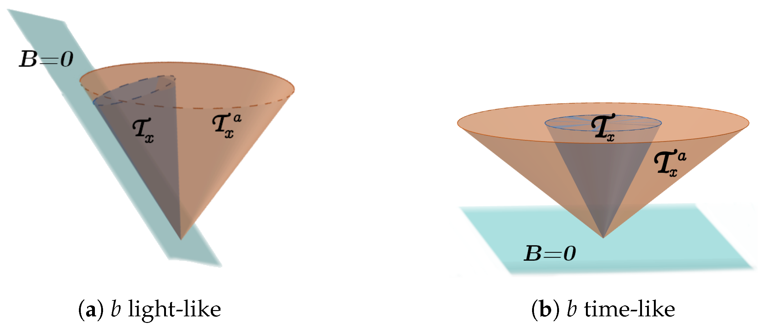
• On the boundary $\partial {\mathcal{T}}_x,$ we must have $L=0$, which implies:

  $$B=-\sqrt{A}\le 0.$$

  (19)
  This leads to the even more interesting conclusion below.
• At any point $x\in M$ of a Randers spacetime, the whole cone ${\mathcal{T}}_x$ lies in the half-space $B<0$:

  $$B\left(\dot{x}\right)<0,\forall \dot{x}\in {\mathcal{T}}_x.$$

  (20)
  In particular, the hyperplane $B=0$ cannot intersect the interior of ${\mathcal{T}}_x$.
  To justify the above, let us first show that $B=0$ cannot occur inside ${\mathcal{T}}_x$. Indeed, if this were the case, then, fixing an arbitrary $u\in {\mathcal{T}}_x\cap \{B=0\}$, the fact that ${\mathcal{T}}_x$ is open in the topology of $T_{x}M\simeq {\mathbb{R}}^4$ guarantees that there must be an entire Euclidean ball centered at u which remains in ${\mathcal{T}}_x$. However, since u is in the hyperplane $B=0$, half of this ball will be contained in the hyperspace $B>0$; in other words, the intersection $\mathcal{C}:={\mathcal{T}}_x\cap \{B>0\}$ is non-empty. By its definition, $\mathcal{C}$ is an open, conic, and convex set and, moreover, by continuity, on the boundary $\partial \mathcal{C}$, we have $B\ge 0$. On the other hand, proceeding as in the first step of the proof of Lemma 2, we find that there must exist a point $\dot{x}\in \partial \mathcal{C}$ where $B\ne 0$. Such a point is, thus, a point of $\partial {\mathcal{T}}_x$, where, in addition, $B>0$, which is in contradiction with the above remark. Therefore, $B=0$ cannot happen in the interior of ${\mathcal{T}}_x$ (but only possibly on its boundary). An immediate consequence of this is that B must have a constant nonzero sign on ${\mathcal{T}}_x$; moreover, this sign is negative.

The last remark points out that inside the future-pointing time-like domain for Randers spacetimes, we always have $\sqrt{s}=-\frac{B}{\sqrt{A}}$. In other words, the restriction $\mathsf{\Psi }:\mathcal{T}\to \mathbb{R}$ (which is relevant to our work) has the expression:

$$\mathsf{\Psi }={(1-\sqrt{s})}^2.$$

The quantities in Theorem 1 are then immediately obtained as:

$$\mathsf{\Psi }-s{\mathsf{\Psi }}^{\prime }=1-\sqrt{s},\sigma =1.$$

(21)

We are now able to prove the following result.

Proposition 2.

A Randers-type deformation of a four-dimensional Lorentzian metric a defines a Finsler spacetime structure if and only if

$$0\le 〈b,b〉<1.$$

If this is the case, then each of its future-pointing time-like cones ${\mathcal{T}}_x$ is the intersection of the cone $A-B^2>0$ with the future-pointing cone of a at x.

Proof. 

→: Assume that L defines a spacetime structure. The fact that, in this case, the cones ${\mathcal{T}}_x$ are the intersections of the cones $\sqrt{A}>-B$ (which is the same as $A>B^2$, taking into account that $B<0$) with ${\mathcal{T}}_x^a$ was already discussed in the first remark above.

• Furthermore, according to Theorem 1, on its future-pointing time-like cones, we must have $\mathsf{\Psi }-s{\mathsf{\Psi }}^{\prime }=1-\sqrt{s}>0$, which is equivalent to $s<1$. Using Lemma 1, this gives

  $$〈b,b〉\le s<1.$$

• To prove the first inequality $〈b,b〉\ge 0$, let us assume that this is not the case, i.e., $〈b,b〉<0$. We will show that, in this case, the hyperplane $B=0$ must intersect ${\mathcal{T}}_x$. To this aim, fix an arbitrary point $x\in M$ and an a-orthonormal basis $\{e_0,e_1,e_2,e_3\}$, with $e_0$ being a-time-like and $e_1$ being collinear to $\tilde{b}$. It follows that $\tilde{b}=\lambda e_1$ for some $\lambda \in {\mathbb{R}}^{*}$. Accordingly, $A=0$ becomes equivalent to ${\left({\dot{x}}^0\right)}^2-{\left({\dot{x}}^1\right)}^2-{\left({\dot{x}}^2\right)}^2-{\left({\dot{x}}^3\right)}^2=0$ and the hyperplane $B=0$ is described by the equation ${\dot{x}}^1=0$. Taking into account (18), it follows that the intersection between this hyperplane and ${\mathcal{T}}_x$ is the region of the three-dimensional cone:

  $${\left({\dot{x}}^0\right)}^2-{\left({\dot{x}}^2\right)}^2-{\left({\dot{x}}^3\right)}^2>0,$$

  (22)

  lying in ${\mathcal{T}}_x^a$ (that is, with ${\dot{x}}^0>0$), which is by far non-empty. This is in contradiction with the fact that the hyperplane $B=0$ cannot intersect ${\mathcal{T}}_x$, as shown above. We conclude that our assumption was false, that is, $〈b,b〉\ge 0$.

←: Assume now that $0\le 〈b,b〉<1$ and let us show that L satisfies the conditions of Theorem 1. Define $\mathcal{T}$ as the intersection of the future-pointing cone bundle ${\mathcal{T}}^a$ with the set $A-B^2>0$, i.e.,

$$(a_{ij}-b_i{b}_j){\dot{x}}^i{\dot{x}}^j>0;$$

(23)

in particular, this entails $s\in (0,1)$. The latter inequality makes it clear that, at each point $x\in M$, the boundary $\partial {\mathcal{T}}_x$ is a quadric. Using the hypothesis $〈b,b〉<1$ and the Lorentzian signature of a, we find that:

$$det(a_{ij}-b_i{b}_j)=det\left(a_{ij}\right)(1-〈b,b〉)<0.$$

This way, the matrix $(a_{ij}-b_i{b}_j)$ can only have $(+,-,-,-)$ or $(-,+,+,+)$ signatures. Moreover, regarding its entries as continuous functions of b, we find that, for $b=0$, the signature of our matrix coincides with that of a, as the matrices themselves coincide. Since the signature cannot change without passing through a zero of the determinant, we find that for all b in the given domain, we still have a $(+,-,-,-)$ signature. In other words, each set ${\mathcal{T}}_x$ is the interior of a convex (and hence, connected) cone.

Moreover, on each fiber ${\mathcal{T}}_x,x\in M$, we have:

• The functions A and $\mathsf{\Psi }$ are, by definition, positive inside $\mathcal{T}$ and, when approaching the boundary of $\mathcal{T}$ (that is, for $s\to 1$), we find that $\mathsf{\Psi }\to 0$ and hence, $L\to 0$. The smoothness of $\mathsf{\Psi }$ follows as the value $s=0$ (which would correspond to $B=0$) cannot appear inside ${\mathcal{T}}_x$. This happens since b is, by hypothesis, non-space-like with respect to a; that is, $B=0$ cannot occur within ${\mathcal{T}}_x^a$ and accordingly cannot occur in ${\mathcal{T}}_x$.
• The conditions in (ii) of Theorem 1 follow immediately using (21).

• Thus, $L=A\mathsf{\Psi }$ defines a Finsler spacetime structure. □

In Figure 2, the possible relative positions of hyperplane $B=0$ with respect to the time-like cones ${\mathcal{T}}_x$ and ${\mathcal{T}}_x^a$ are displayed, with the same color meaning as in Figure 1.

Remark 4.

1.

The result above extends those in [42] by taking into consideration the case when b is a-space-like and actually proving that this never defines a Randers spacetime.

2.

A very recent article1, [21], proposed a modification of the standard Randers metric. With our above notations and signature convention $(+,-,-,-)$, on the set of interest $A>0$, this reads:

$$L=ϵ(\sqrt{A}-{\left|B\right|)}^2.$$

(24)

This is a very interesting extension, as it removes the request that B should be strictly negative inside ${\mathcal{T}}_x$. Thus, for modified Randers metrics (24), the restriction $〈b,b〉\ge 0$ (which was motivated precisely by the fact that once crossing the hyperplane $B=0$, B changes sign) is no longer necessary. Moreover, on regions where $L>0$ and $A>0$ (in which the cones ${\mathcal{T}}_x$ must be contained), we have $\mathsf{\Psi }={(1-\sqrt{s})}^2$ just as above (with the only difference that, in the definition of s, we no longer have $\left|B\right|=-B$). Thus, a completely similar reasoning shows that (24) leads to a well-defined spacetime structure if and only if $〈b,b〉<1$. This is consistent with the result in [21].

4.3. Bogoslovsky–Kropina Metrics $L=A^{1-q}{B}^{2q}$

We will leave aside the case when $q=0$, as it is trivial.

Proposition 3.

A Bogoslovsky–Kropina metric $L=A^{1-q}{B}^{2q}$ with $q\ne 0$ defines a spacetime structure if and only if one of the following occurs:

(i)

$〈b,b〉>0$ and $q\in [-1,1).$ In this case, the future-pointing cones of L coincide with those of A.

(ii)

$〈b,b〉=0$ and $q\in (-1,1).$ In this case, the future-pointing cones of L coincide with those of A.

(iii)

$〈b,b〉<0$ and $q\in (0,1)$. In this case, the future-pointing cones of L are obtained by intersecting the future-pointing cones of A with the half-space $B>0$.

Proof. 

The Finsler function is expressed as $L=A{s}^q$, which means that $\mathsf{\Psi }$ has the expression:

$$\mathsf{\Psi }\left(s\right):=s^q.$$

(25)

• $\to :$ Assume that L defines a spacetime structure and let us first identify the future-pointing cones ${\mathcal{T}}_x$ of L, together with the domain of the definition of $\mathsf{\Psi }$.

Fix $x\in M$. As we have seen above, for any $(\alpha ,\beta )$-metric, the cone ${\mathcal{T}}_x$ must be contained in ${\mathcal{T}}_x^a$. Moreover, in our specific case, boundary points must be either on the cone $A=0$ or in the plane $B=0$. Thus:

1.

If b is non-space-like with respect to a, then $B=0$ cannot happen inside ${\mathcal{T}}_x^a$ (it can, in the worst case, when b is a-light-like, happen on its boundary). In this case, we thus have ${\mathcal{T}}_x={\mathcal{T}}_x^a$; moreover, the reverse Cauchy–Schwarz inequality tells us that $s\ge 〈b,b〉$, with equality for $\dot{x}\sim \tilde{b}$. In other words, the minimum value $s_0=〈b,b〉$ is always attained on the closure of ${\mathcal{T}}_x$.

2.

If b is a-space-like, then points with $B=0$ will always exist inside ${\mathcal{T}}_x^a$. We note that, in order to have a finite limit for $L=A^{1-q}{B}^q$ as we approach the hyperplane $B=0$, we must necessarily have:

$$q>0.$$

(26)

In this case, the cone ${\mathcal{T}}_x$ will be the region of the cone ${\mathcal{T}}_x^a$ situated in the half-space $B>0$ and s will tend to zero as we approach the boundary points with $B=0$.

3.

On the other hand, as shown above, the boundary of each cone ${\mathcal{T}}_x$ of any $(\alpha ,\beta )$-metric spacetime must contain at least one point where $B\ne 0$. In our case, this means that there will always be at least one boundary point satisfying $A=0$, i.e., we necessarily have in ${\mathcal{T}}_x$, values $s\to \infty$.

• Briefly: in any case, $\mathsf{\Psi }$ is defined on the entire interval:

  $$s\in (s_0,\infty ),s_0:=max\{〈b,b〉,0\}.$$

  (27)

• Having identified the function $\mathsf{\Psi }$, we are now ready to rewrite, in our case, the conditions in Theorem 1.

• Since, inside the above-identified cones ${\mathcal{T}}_x$, we obviously have $A>0$ and $\mathsf{\Psi }>0$, where $\mathsf{\Psi }$ is smooth, in order to check these conditions, we must impose that when approaching any point of the boundary ${\mathcal{T}}_x$, we should have $L=A^{1-q}{B}^q\to 0$. This immediately implies:

  $$q<1.$$

  (28)
• The first inequality $\mathsf{\Psi }-s{\mathsf{\Psi }}^{\prime }>0$ becomes $s^q(1-q)>0$, i.e., it is equivalent to the same inequality $q<1$.

• Noting that $\sigma :=s^q{(q-1)}^2,$ the second inequality (16) reads $(s-〈b,b〉){\displaystyle \frac{q}{s}}>-1$, which, taking into account that $s>0$, is equivalent to

  $$\left(q+1\right)s>〈b,b〉q.$$

  (29)

To solve this inequality, we note that its left hand side is linear in s; hence, it is necessary and sufficient to check its non-strict version at the endpoints of the interval $(s_0,\infty )$ (with just a bit of extra attention to $q=-1$, for which this linear function identically vanishes). Thus:

• If $〈b,b〉>0$, then at the lower bound $s_0=〈b,b〉>0$, the (non-strict) inequality (29) is identically satisfied. Imposing it for $s\to \infty$, we find:

  $$q\ge -1,$$

  (30)

  which proves the necessity of condition (i) in our statement.
• If $〈b,b〉=0,$ then for $s_0=0$, the (non-strict) inequality (29) is identically satisfied. Imposing it for $s\to \infty$, we find:

  $$q\ge -1.$$

  (31)
  Yet, we note that $q=-1$ cannot actually happen, as it would lead to equality in (29) for all s, which proves the necessity of condition (ii) in our statement.
• If $〈b,b〉<0$, then for $s\to \infty$, we find $q>-1$, whereas the lower bound $s_0=0$ gives $q\ge 0$, proving the necessity of condition (iii).

• ←: Assuming one of the situations (i)–(iii) happens, then the conditions in Theorem 1 are immediately satisfied on the said cones by $\mathsf{\Psi }:(s_0,\infty )\to \mathbb{R},\mathsf{\Psi }\left(s\right)=s^q$. Hence, L defines a spacetime structure. □

4.4. Generalized m-Kropina (VGR) Metrics

These are given by:

$$L(x,\dot{x})=A{s}^{-p}{\left(k+ms\right)}^{p+1}=B^{-2p}{\left(kA+m{B}^2\right)}^{p+1},$$

(32)

where $p,k,m\in \mathbb{R}$ are constants. As $k=0$ gives a degenerate metric and $m=0$ provides the already discussed Bogoslovsky–Kropina class, we will assume here that $k,m\ne 0.$ The corresponding function $\mathsf{\Psi }$ is given by:

$$\mathsf{\Psi }\left(s\right)={\displaystyle \frac{{\left(k+ms\right)}^{p+1}}{s^p}}.$$

Proposition 4.

The generalized m-Kropina metric $L(x,\dot{x})=A{s}^{-p}{\left(k+ms\right)}^{p+1}$ defines a Finsler spacetime metric if and only if $k>0,m<0,$ and one of the following situations occurs:

(i)

$〈b,b〉\ge 0\mathrm{and}p\in (-1,1]$.

In this case, the future-pointing time-like cones of L are the connected components of the cones $kA+m{B}^2>0$ contained in the future-pointing time-like cones ${\mathcal{T}}_x^a$.

(ii)

$〈b,b〉<0\mathrm{and}p\in (-1,0)$.

In this case, the future-pointing time-like cones of L are regions of the the cones $kA+m{B}^2>0$ lying both in the future-pointing time-like cones ${\mathcal{T}}_x^a$ and in the half-space $B>0$.

Proof. 

$\to :$ Assume L defines a Finsler spacetime structure. Let us first make some general remarks on the future-pointing time-like cones ${\mathcal{T}}_x$, that hold regardless of the causal character of b. To this aim, fix an arbitrary $x\in M$.

The latter equality in (32) reveals that the only boundary points $\dot{x}\in \partial {\mathcal{T}}_x$ where $B\ne 0$ are in the set $kA+m{B}^2=0,$ which corresponds to $s=-{\displaystyle \frac{k}{m}}$. Since such boundary points must exist and lead to the finite value $L=0$ and, on the other hand, they must correspond to strictly positive values of s, we obtain, respectively:

$$p+1>0,-{\displaystyle \frac{k}{m}}>0.$$

(33)

The latter relation points out that k and m must have opposite signs. To see precisely what these signs are, we evaluate the first condition in Theorem 1 (ii):

$$\mathsf{\Psi }-s{\mathsf{\Psi }}^{\prime }>0\iff k(p+1){(k+ms)}^p{s}^{-p}>0,$$

(34)

which shows that only viable variant is:

$$k>0,m<0,$$

(35)

as claimed. This means that the inequality $k+ms>0$ is equivalent to $s<-{\displaystyle \frac{k}{m}}$, which gives, for $\dot{x}\in {\mathcal{T}}_x$:

$$s\in I\subset \left(0,-{\displaystyle \frac{k}{m}}\right),$$

where the upper bound $-{\displaystyle \frac{k}{m}}$ of the interval I is sharp. The lower bound, however, depends on the a-causal character of b.

The second condition in Theorem 1 (ii) becomes:

$$\rho {\displaystyle \frac{{\sigma }^{\prime }}{\sigma }}>-1\iff \left(〈b,b〉m-kp+k\right)s+〈b,b〉kp>0.$$

(36)

This holds for every s corresponding to $\dot{x}\in {\mathcal{T}}_x$ if and only if it holds (non-strictly) at the bounds of the interval I.

At the upper bound $s\to -{\displaystyle \frac{k}{m}}$, this gives:

$$\left(p-1\right)\left(〈b,b〉m+k\right)\le 0.$$

Taking into account $s\ge 〈b,b〉$ together with $m<0$, it follows that

$$k+m〈b,b〉\ge k+ms>0.$$

(37)

Therefore, we must have $p-1\le 0$ and, all in all,

$$p\in (-1,1].$$

(38)

Another important consequence of (37) is that it ensures that the cones $kA+m{B}^2>0$ are, indeed, convex cones. This is seen as the matrix $(k{a}_{ij}+m{b}_i{b}_j)$ has the determinant $k^{4}det\left(a\right)(1+\frac{m}{k}〈b,b〉)<0$. A quick similar reasoning to the one in the Randers subsection shows that its signature is the same as the one of a, i.e., $(+,-,-,-)$. In other words, $kA+m{B}^2>0$ is the interior of a convex cone. Moreover, as $kA>kA+m{B}^2$, this cone is completely contained in the cone $A>0$.

It remains to evaluate (36) at the lower bound for s. Since this depends on the sign of $〈b,b〉$, we distinguish two major cases:

1.

Assume $〈b,b〉\ge 0$. Then, $B=0$ cannot happen inside the future-pointing time-like cones of a, and hence cannot occur in the Finslerian ones ${\mathcal{T}}_x$. Thus, in this case, each of the cones ${\mathcal{T}}_x$ is the connected component of the convex cone:

$$kA+m{B}^2>0$$

(39)

contained in ${\mathcal{T}}_x^a$. In this case, a quick check shows that:

$$(k{a}_{ij}+m{b}_i{b}_j){\tilde{b}}^i{\tilde{b}}^j=〈b,b〉(k+m〈b,b〉)\ge 0,$$

(40)

which means that one of the vectors $\tilde{b}$ or $-\tilde{b}$ belongs to ${\overline{\mathcal{T}}}_x$. In either case, we find that the corresponding value $s_0=〈b,b〉$ is attained on the closure of ${\mathcal{T}}_x$ and it represents the lower bound for $s\in I$.

At this lower bound, inequality (36) reduces to:

$$〈b,b〉(k+m〈b,b〉)\ge 0$$

and is identically satisfied for any value of $p\in (-1,1]$.

2.

Suppose $〈b,b〉<0$. Then, the hyperplane $B=0$ has common points with the cone $kA+m{B}^2>0$. However, points with $B=0$ are either singular points for L (if $p>0$), or null cone points if $p<0$. Obviously, the only viable situation is the second one, namely:

$$p\in (-1,0).$$

(41)

Knowing this, evaluation of (36) at the lower bound of the interval for s, which is in this case $s=0$, gives:

$$〈b,b〉kp\ge 0$$

(42)

which always happens, as $〈b,b〉<0,p<0,k>0$.

The future-pointing time-like cones of L are then the intersections of the cone $kA+m{B}^2>0$ with the future-pointing cones ${\mathcal{T}}_x^a$ and the half-space $B>0$.

• $\leftarrow :$ Assuming $k>0$ and $m<0$, then the matrix $(k{a}_{ij}+m{b}_i{b}_j)$ has a Lorentzian signature $(+,-,-,-)$, meaning that the set $kA+m{B}^2>0$ is a convex cone, which is, moreover, contained in the cone $A>0$. Then, assuming one of the situations (i) or (ii) holds, one can immediately check the conditions of Theorem (1) for the specified ${\mathcal{T}}_x$ (note that statement (ii) in the theorem is equivalent to (34) and (36)). □

4.5. Exponential Metrics $L=A{e}^{P\left(s\right)}$

Here, $P=P\left(s\right)$ denotes an arbitrary smooth function for all s in the interval $I=(max\{0,〈b,b〉\},\infty )$. Since $e^{P\left(s\right)}$ has no zeros, the cone ${\mathcal{T}}_x$ is the entire cone of a, and, accordingly, the domain of s is the entire interval I above.

Proposition 5.

The exponential metric $L=A{e}^{P\left(s\right)}$ defines a Finsler spacetime structure if and only if:

$$\begin{array}{ccc}& & \underset{s\to \infty }{lim}{\displaystyle \frac{e^{P\left(s\right)}}{s}}=0,\hfill \\ & 1-s{P}^{\prime }>0,& 1-s{P}^{\prime }>\left(s-〈b,b〉\right)\left(s{\left(P^{\prime }\right)}^2+2s{P}^{″}+P^{\prime }\right),\forall s\in I.\hfill \end{array}$$

(43)

• If this is the case, then the future-pointing time-like cones of L coincide with those of the Lorentzian metric A.

Proof. 

To justify the above statement, we note that, in this case, L and A always have the same sign, which means that the future-pointing time-like cones of L and A must be the same. Moreover,

$$\mathsf{\Psi }\left(s\right)=e^{P\left(s\right)};$$

therefore, the first relation (43) is equivalent to $\underset{\dot{x}\to \partial T_x}{lim}\left(A\mathsf{\Psi }\right)=0$ and the second one is equivalent to $\mathsf{\Psi }-s{\mathsf{\Psi }}^{\prime }>0,$ whereas a brief calculation using $\sigma =e^P{(1-s{P}^{\prime })}^2$ reveals that the latter one is just $\rho {\displaystyle \frac{{\sigma }^{\prime }}{\sigma }}>-1.$ □

Example 1.

A concrete example, which resembles the so-called Maxwell–Boltzmann distribution function in the kinetic theory of gases, is obtained by considering an arbitrary metric a on $M,$ together with a time-like 1-form $b\in {\Omega }_1\left(M\right)$ and

$$\mathsf{\Psi }:[〈b,b〉,\infty )\to {\mathbb{R}}_{+},\mathsf{\Psi }\left(s\right)=e^{k-\frac{{〈b,b〉}^2}{2s^2}},$$

where $k>0$ is a constant. The first two conditions in (43) are immediately checked. Besides, a brief calculation shows that the third one is equivalent to

$$s^4+〈b,b〉s^3+5{〈b,b〉}^2{s}^2-{〈b,b〉}^4>0.$$

The latter is trivially satisfied at $s=〈b,b〉>0$ and the left hand side is a monotonically increasing function on $(0,\infty )$; hence, the inequality holds for all $s\in [〈b,b〉,\infty ).$

5. Isometries of $(\mathbf{\alpha },\mathbf{\beta })$-Metric Spacetimes

An isometry of a pseudo-Finsler space is, [28], a diffeomorphism $\phi :M\to M$ whose natural lift $T\phi :TM\to TM$ leaves L invariant. Leaving aside possible discrete symmetries, we will turn our attention to one-parameter Lie groups of isometries. Their generators, known as Finslerian Killing vector fields $\xi ={\xi }^i{\partial }_i\in \mathcal{X}\left(M\right)$, are given by the equation:

$${\xi }^C\left(L\right)=0,$$

(44)

where ${\xi }^C={\xi }^i{\partial }_i+{\xi }_{,j}^i{\dot{x}}^j{\dot{\partial }}_i$ is the complete lift of $\xi$ to $TM.$

In particular, for $\left(\alpha ,\beta \right)$-metric functions $L=A\mathsf{\Psi }\left(s\right)$, with $s={\displaystyle \frac{B^2}{A}},$ the Killing vector condition reads ${\xi }^C\left(A\right)\mathsf{\Psi }+A{\mathsf{\Psi }}^{\prime }{\xi }^C\left(s\right)=0,$ equivalently:

$${\xi }^C\left(A\right)\left(\mathsf{\Psi }-s{\mathsf{\Psi }}^{\prime }\right)+2{\mathsf{\Psi }}^{\prime }B{\xi }^C\left(B\right)=0,$$

(45)

where

$${\xi }^C\left(A\right)=\left({\mathfrak{L}}_{\xi }{a}_{ij}\right){\dot{x}}^i{\dot{x}}^j,{\xi }^C\left(B\right)=\left({\mathfrak{L}}_{\xi }{b}_i\right){\dot{x}}^i$$

are polynomial expressions of degree two and one, respectively, in $\dot{x}.$

Particular case: trivial symmetries. Assume L is non-Riemannian, that is, ${\mathsf{\Psi }}^{\prime }\left(s\right)\ne 0$ at least on some interval $I_0\subset I.$ If $\xi$ is a Killing vector field of $L,$ then

$${\xi }^C\left(A\right)=0\iff {\xi }^C\left(B\right)=0,$$

which, differentiating with respect to $\dot{x},$ gives:

$${\mathfrak{L}}_{\xi }a=0\iff {\mathfrak{L}}_{\xi }b=0.$$

In other words, if $\xi$ is a Killing vector field of $a,$ then it is a Killing vector field of any $\left(\alpha ,\beta \right)$-metric $L=A\mathsf{\Psi }$ with 1-form $b\in {\Omega }_1\left(M\right)$ invariant under the flow of $\xi$, regardless of the form of $\mathsf{\Psi }.$

We will call Killing vectors of L obeying any of the equivalent conditions ${\mathfrak{L}}_{\xi }a=0$ or ${\mathfrak{L}}_{\xi }b=0$ trivial symmetries of L.

Nontrivial symmetries. In the following, let us explore which $\left(\alpha ,\beta \right)$-metrics admit nontrivial symmetries. We find the following result, which is valid for all pseudo-Finsler $\left(\alpha ,\beta \right)$ metrics, independently of their signature.

Theorem 2.

A non-Riemannian $\left(\alpha ,\beta \right)$ pseudo-Finsler function $L=A\mathsf{\Psi }$ admits nontrivial Killing vector fields if and only if:

$$\mathsf{\Psi }=\left\{\begin{array}{cc}c{s}^{\frac{{\mu }_1}{{\mu }_1-2{\lambda }_2}}{|{\mu }_{2}s+{\mu }_1-2{\lambda }_2|}^{-\frac{2{\lambda }_2}{{\mu }_1-2{\lambda }_2}},\hfill & \mathit{if}{\mu }_1\ne 2{\lambda }_2\hfill \\ cs{e}^{-\frac{2{\lambda }_2}{{\mu }_{2}s}},\hfill & \mathit{if}{\mu }_1=2{\lambda }_2,{\mu }_2\ne 0\hfill \end{array}\right.$$

(46)

for some smooth functions $c,{\lambda }_2,{\mu }_1,{\mu }_2$ of x only, and there exist solutions $\xi \in \mathcal{X}\left(M\right)$ of the equations

$${\xi }^C\left(B\right)=\kappa {\lambda }_{2}B,{\xi }^C\left(A\right)=\kappa \left({\mu }_{1}A+{\mu }_2{B}^2\right),$$

(47)

for some $\kappa =\kappa \left(x\right)$ which does not identically vanish. If this is the case, the nontrivial Killing vectors of L are precisely the solutions of (47).

Proof. 

$\to :$ Assume that L admits a nontrivial Killing vector field $\xi \in \mathcal{X}\left(M\right),$ i.e., ${\xi }^C\left(L\right)=0,$ but ${\xi }^C\left(A\right)$ does not identically vanish.

Fix $x\in M$ and let us restrict our attention to an open, conic subset of ${\mathcal{T}}_x$ where ${\xi }^C\left(A\right)\ne 0$. For these, we can rewrite the Killing Equation (45) as:

$${\displaystyle \frac{B{\xi }^C\left(B\right)}{{\xi }^C\left(A\right)}}={\displaystyle \frac{s{\mathsf{\Psi }}^{\prime }-\mathsf{\Psi }}{2{\mathsf{\Psi }}^{\prime }}}={\displaystyle \frac{1}{2}}\left(s-{\displaystyle \frac{\mathsf{\Psi }}{{\mathsf{\Psi }}^{\prime }}}\right).$$

(48)

In particular, the latter expression must be equal to a ratio of two homogeneous polynomial expressions of degree two in $\dot{x}.$ However, on the other hand, it is a function of $B^2$ and $A;$ the only such possibility is:

$${\displaystyle \frac{s{\mathsf{\Psi }}^{\prime }-\mathsf{\Psi }}{2{\mathsf{\Psi }}^{\prime }}}={\displaystyle \frac{{\lambda }_{1}A+{\lambda }_2{B}^2}{{\mu }_{1}A+{\mu }_2{B}^2}},$$

(49)

for some ${\lambda }_1,{\lambda }_2,{\mu }_1,{\mu }_2$ depending on x only. Depending on whether ${\lambda }_1,{\mu }_1$ vanish or not, we distinguish four situations:

1.

${\lambda }_1,{\mu }_1=0.$ In this case, ${\displaystyle \frac{s{\mathsf{\Psi }}^{\prime }-\mathsf{\Psi }}{2{\mathsf{\Psi }}^{\prime }}}={\displaystyle \frac{{\lambda }_2}{{\mu }_2}}=:\kappa \left(x\right)$ only. Integration of this equation gives:

$$\mathsf{\Psi }=c\left(s-2\kappa \right),c=c\left(x\right),$$

which means that $L=A\mathsf{\Psi }=c\left(B^2-2\kappa A\right)$ is actually pseudo-Riemannian.

2.

${\lambda }_1=0,{\mu }_1\ne 0.$ In this situation, the first equality (48) gives, after simplification by B,

$${\displaystyle \frac{{\xi }^C\left(B\right)}{{\xi }^C\left(A\right)}}={\displaystyle \frac{{\lambda }_{2}B}{{\mu }_{1}A+{\mu }_2{B}^2}}.$$

We note that, on the right hand side, on the one hand, we must have ${\lambda }_2\ne 0$ (otherwise we only get trivial symmetries ${\xi }^C\left(B\right)=0$) and, on the other hand, the numerator and the denominator must be given by relatively prime polynomials; in the contrary case, A would admit B as a factor, which is not possible, since its $\dot{x}$-Hessian $\left(2a_{ij}\right)$ is nondegenerate. However, then B must divide ${\xi }^C\left(B\right)$, that is,

$${\xi }^C\left(B\right)=\kappa {\lambda }_{2}B,$$

where, given that $degB=deg{\xi }^C\left(B\right)=1,$ we must have $\kappa =\kappa \left(x\right)$ only. Accordingly,

$${\xi }^C\left(A\right)=\kappa \left({\mu }_{1}A+{\mu }_2{B}^2\right).$$

The functions $\mathsf{\Psi }$ corresponding to such symmetries are then obtained from (49), which in our case reads

$$s-\frac{\mathsf{\Psi }}{{\mathsf{\Psi }}^{\prime }}=\frac{2{\lambda }_{2}s}{{\mu }_1+{\mu }_{2}s}$$

(50)

and can be directly integrated to give

$$\mathsf{\Psi }=cexp\left(\int {\displaystyle \frac{\left({\mu }_1+s{\mu }_2\right)ds}{{\mu }_2{s}^2+\left({\mu }_1-2{\lambda }_2\right)s}}\right).$$

(51)

Calculation of the integral then leads to (46). We note that the situation ${\mu }_1-2{\lambda }_2=0$, ${\mu }_2=0$ is not possible, as it would lead in (50) to $\frac{\mathsf{\Psi }}{{\mathsf{\Psi }}^{\prime }}=0.$

3.

${\lambda }_1\ne 0,{\mu }_1=0.$ This gives ${\displaystyle \frac{B{\xi }^C\left(B\right)}{{\xi }^C\left(A\right)}}={\displaystyle \frac{{\lambda }_{1}A+{\lambda }_2{B}^2}{{\mu }_2{B}^2}}$ and, equivalently,

$$B^3{\mu }_2{\xi }^C\left(B\right)={\xi }^C\left(A\right)\left({\lambda }_{1}A+{\lambda }_2{B}^2\right).$$

(52)

This implies that B must divide ${\lambda }_{1}A+{\lambda }_2{B}^2$, since ${\xi }^C\left(A\right)$ is of degree two and hence it cannot “swallow” more than a factor of $B^2$ of the $B^3$ from the left hand side. This in turn implies that B divides $A,$ thus leading to a degenerate $\dot{x}$-Hessian for A, which is impossible.

4.

${\lambda }_1,{\mu }_1\ne 0.$ In this case, we have:

$${\displaystyle \frac{B{\xi }^C\left(B\right)}{{\xi }^C\left(A\right)}}={\displaystyle \frac{{\lambda }_{1}A+{\lambda }_2{B}^2}{{\mu }_{1}A+{\mu }_2{B}^2}}.$$

(53)

The ratio on the right hand side is either irreducible or a function of x only. This is derived as follows. Assuming that it can be simplified by a first degree factor, then both ${\lambda }_{1}A+{\lambda }_2{B}^2$ and ${\mu }_{1}A+{\mu }_2{B}^2$ must be decomposable; in particular, they must have degenerate $\dot{x}$-Hessians, i.e.,

$$det\left({\lambda }_1{a}_{ij}+{\lambda }_2{b}_i{b}_j\right)=det\left({\mu }_1{a}_{ij}+{\mu }_2{b}_i{b}_j\right)=0.$$

Using Lemma A1 (see Appendix A), that is ${\lambda }_1^{4}deta\left(1+{\displaystyle \frac{{\lambda }_2}{{\lambda }_1}}〈b,b〉\right)=$${\mu }_1^{4}deta\left(1+{\displaystyle \frac{{\mu }_2}{{\mu }_1}}〈b,b〉\right)=0,$ leads to

$${\displaystyle \frac{{\lambda }_2}{{\lambda }_1}}={\displaystyle \frac{{\mu }_2}{{\mu }_1}}.$$

The latter actually means that the ratio ${\displaystyle \frac{{\lambda }_{1}A+{\lambda }_2{B}^2}{{\mu }_{1}A+{\mu }_2{B}^2}}={\displaystyle \frac{{\lambda }_1}{{\mu }_1}}$ depends on x only (i.e., it is actually simplified by a second degree factor, not a first degree one, as assumed).

Thus, we only have two possibilities:

(a)

${\displaystyle \frac{{\lambda }_{1}A+{\lambda }_2{B}^2}{{\mu }_{1}A+{\mu }_2{B}^2}}=\kappa \left(x\right)$, that is, ${\displaystyle \frac{s{\mathsf{\Psi }}^{\prime }-\mathsf{\Psi }}{2{\mathsf{\Psi }}^{\prime }}}=\kappa$, which, by a similar reasoning to Case 1, entails that L is actually pseudo-Riemannian.

(b)

${\displaystyle \frac{{\lambda }_{1}A+{\lambda }_2{B}^2}{{\mu }_{1}A+{\mu }_2{B}^2}}$ is irreducible. In this case, from (53), we find that B must either divide ${\xi }^C\left(A\right)$ (but, then, ${\displaystyle \frac{{\lambda }_{1}A+{\lambda }_2{B}^2}{{\mu }_{1}A+{\mu }_2{B}^2}}={\displaystyle \frac{B{\xi }^C\left(B\right)}{{\xi }^C\left(A\right)}}$ would equal a ratio of first degree polynomials, which contradicts the irreducibility assumption) or it must divide ${\lambda }_{1}A+{\lambda }_2{B}^2$, which, taking into account that A and B are always relatively prime, leads to ${\lambda }_1=0,$ in contradiction with the hypothesis ${\lambda }_1\ne 0.$

Therefore, there are no properly Finslerian functions L with ${\lambda }_1,{\mu }_1\ne 0.$

We conclude that the only valid possibility is Case 2, thus giving the statement of the theorem.

• $\leftarrow :$ Conversely, assuming that $\xi$ and $\mathsf{\Psi }$ satisfy (47) and (46), a direct computation shows that ${\xi }^C\left(L\right)={\xi }^C\left(A\right)\mathsf{\Psi }+A{\mathsf{\Psi }}^{\prime }{\xi }^C\left(s\right)=0,$ and hence $\xi$ is a Killing vector for $L=A\mathsf{\Psi }.$

If L is non-Riemannian, these symmetries are always nontrivial. This is seen by the fact that ${\xi }^C\left(A\right)=0$ is only possible when ${\mu }_1={\mu }_2=0$, which is, $\mathsf{\Psi }=const.$, corresponding to a Lorentzian metric. □

The above result gives necessary and sufficient conditions for an $\left(\alpha ,\beta \right)$-metric to admit nontrivial symmetries. There remains, of course, the question whether such metrics really exist. To show that the answer is affirmative, we present below a concrete example.

Example 2.

Nontrivial symmetries of a Bogoslovsky–Kropina spacetime metric.Consider, on $M={\mathbb{R}}^4,$ a conformal deformation a of the Minkowski metric $\eta =diag(1,-1,-1,-1)$ and a light-like 1-form b, as follows:

$$a=e^{2q{x}^0}\eta ,b=e^{\left(q-1\right)x^0}\left(d{x}^0+d{x}^1\right),$$

where $q\in \left(0,1\right)$ is arbitrarily fixed. With these data, the Bogoslovsky-type metric:

$$L=A{s}^q,s={\displaystyle \frac{B^2}{A}}={\displaystyle \frac{{\left(b\left(\dot{x}\right)\right)}^2}{a\left(\dot{x},\dot{x}\right)}}$$

is a nontrivial Finsler spacetime function, whose $\mathsf{\Psi }\left(s\right)=s^q,$ fits into class (46) (for ${\lambda }_2=q-1,{\mu }_1=2q,{\mu }_2=0,\kappa =c=1$).

We take $\xi$ as the time translation generator $\xi ={\partial }_0,$ which gives:

$${\xi }^C={\partial }_0.$$

Then, using $A=e^{2q{x}^0}{\eta }_{ij}{\dot{x}}^i{\dot{x}}^j,$ $B=e^{\left(q-1\right)x^0}\left({\dot{x}}^0+{\dot{x}}^1\right),$ we immediately find:

$${\xi }^C\left(A\right)=2qA\ne 0,{\xi }^C\left(B\right)=\left(q-1\right)B,$$

which are precisely the conditions in (47). Therefore, $\xi$ is a nontrivial Killing vector field for L.

6. Conclusions

Among all possible Finsler metrics, the class of $(\alpha ,\beta )$-metrics is of particular interest, since it allows for numerous applications and explicit calculations. Up to now, it was not known how to identify $(\alpha ,\beta )$-Finsler spacetimes in general. They have potential applications in physics, and in particular in gravitational physics.

In this article, we identified the necessary and sufficient conditions such that an $(\alpha ,\beta )$-Finsler metric defines a Finsler spacetime in Theorem 1; these are the conditions that ensure a Lorentzian signature inside a convex cone with null boundary, in each tangent space. As we demonstrated afterwards, this enables us to find the best candidates for physical applications belonging to different subclasses of $(\alpha ,\beta )$-metrics. For Randers metrics, we found that the defining 1-form must be non-space-like and with bounded norms with respect to the pseudo-Riemannian metric (Proposition 2). For Bogoslovsky–Kropina metrics, the value of the power parameter is constrained (Proposition 3). For generalized m-Kropina and exponential type metrics, we provided simple necessary and sufficient Finsler spacetime constraints in Propositions 4 and Proposition 5, respectively.

Moreover, we investigated the existence of isometries of $(\alpha ,\beta )$-metrics. Surprisingly, it turned out that there can exist isometries of a Finsler metric which are not isometries of the metric2 a, as we pointed out in Theorem 2 and, subsequently, in a concrete example. The physical consequences of the existence of these isometries still must be determined. This paper is meant as a starting point for—we hope—numerous research works. Here are just some ideas we want to pursue in the near future:

1.

To use $(\alpha ,\beta )$-metrics with given symmetries as ansatzes for solving the Finslerian gravitational field equation in [3,32,42].

2.

To calculate and understand the precise physical interpretation of the various non-Riemannian notions such as Berwald or Landsberg curvature (see, e.g., [47]), with a special focus on spacetimes with $(\alpha ,\beta )$-metrics. We conjecture that these non-Riemannian quantities could account for at least a part of the observed dark energy phenomenology.

3.

In light of the above, it will be important to construct some non-trivial Ricci flat Finsler $(\alpha ,\beta )$-metric spacetimes with some nonzero non-Riemannian quantities. Some interesting Ricci flat Finsler spacetimes have been constructed, although they are not in an $(\alpha ,\beta )$-form, see, e.g., [48].

4.

To construct the most general spatially spherically symmetric and the most general cosmologically symmetric spacetimes of $(\alpha ,\beta )$-metric type, whose underlying Lorentzian metrics do not possess such symmetries.

5.

To completely classify $(\alpha ,\beta )$-metrics which lead to well-defined Finsler spacetimes, for which the underlying pseudo-Riemannian metric a has a non-Lorentzian signature.

References

- Pfeifer, C. Finsler spacetime geometry in Physics. Int. J. Geom. Meth. Mod. Phys. 2019, 16, 1941004. [Google Scholar] [CrossRef]
- Saridakis, E.N.; Lazkoz, R.; Salzano, V.; Moniz, P.V.; Capozziello, S.; Jiménez, J.B.; De Laurentis, M.; Olmo, G.J. Modified Gravity and Cosmology: An Update by the CANTATA Network; Springer: Cham, Switzerland, 2021. [Google Scholar]
- Hohmann, M.; Pfeifer, C.; Voicu, N. Relativistic kinetic gases as direct sources of gravity. Phys. Rev. 2020, D101, 024062. [Google Scholar] [CrossRef]
- Addazi, A.; Alvarez-Muniz, J.; Batista, R.A.; Amelino-Camelia, G.; Antonelli, V.; Arzano, M.; Asorey, M.; Atteia, J.-L.; Bahamonde, S.; Bajardi, F.; et al. Quantum gravity phenomenology at the dawn of the multi-messenger era—A review. Prog. Part. Nucl. Phys. 2022, 125, 103948. [Google Scholar] [CrossRef]
- Lobo, I.P.; Pfeifer, C. Reaching the Planck scale with muon lifetime measurements. Phys. Rev. D 2021, 103, 106025. [Google Scholar] [CrossRef]
- Amelino-Camelia, G.; Barcaroli, L.; Gubitosi, G.; Liberati, S.; Loret, N. Realization of doubly special relativistic symmetries in Finsler geometries. Phys. Rev. D 2014, 90, 125030. [Google Scholar] [CrossRef]
- Kostelecký, A. Riemann-Finsler geometry and Lorentz-violating kinematics. Phys. Lett. B 2011, 701, 137–143. [Google Scholar] [CrossRef]
- Shreck, M. Classical Lagrangians and Finsler structures for the nonminimal fermion sector of the Standard-Model Extension. Phys. Rev. 2016, D93, 105017. [Google Scholar] [CrossRef]
- Kostelecký, V.A.; Russell, N.; Tso, R. Bipartite Riemann–Finsler geometry and Lorentz violation. Phys. Lett. 2012, B716, 470–474. [Google Scholar] [CrossRef]
- Gibbons, G.; Gomis, J.; Pope, C. General very special relativity is Finsler geometry. Phys. Rev. D 2007, 76, 081701. [Google Scholar] [CrossRef]
- Cohen, A.G.; Glashow, S.L. Very special relativity. Phys. Rev. Lett. 2006, 97, 021601. [Google Scholar] [CrossRef]
- Fuster, A.; Pabst, C. Finsler pp-waves. Phys. Rev. 2016, D94, 104072. [Google Scholar] [CrossRef]
- Fuster, A.; Pabst, C.; Pfeifer, C. Berwald spacetimes and very special relativity. Phys. Rev. 2018, D98, 084062. [Google Scholar] [CrossRef]
- Elbistan, M.; Zhang, P.M.; Dimakis, N.; Gibbons, G.W.; Horvathy, P.A. Geodesic motion in Bogoslovsky-Finsler spacetimes. Phys. Rev. D 2020, 102, 024014. [Google Scholar] [CrossRef]
- Bouali, A.; Chaudhary, H.; Hama, R.; Harko, T.; Sabau, S.V.; Martín, M.S. Cosmological tests of the osculating Barthel–Kropina dark energy model. Eur. Phys. J. C 2023, 83, 121. [Google Scholar] [CrossRef]
- Gibbons, G.W.; Herdeiro, C.A.R.; Warnick, C.M.; Werner, M.C. Stationary Metrics and Optical Zermelo-Randers-Finsler Geometry. Phys. Rev. D 2009, 79, 044022. [Google Scholar] [CrossRef]
- Werner, M.C. Gravitational lensing in the Kerr-Randers optical geometry. Gen. Rel. Grav. 2012, 44, 3047–3057. [Google Scholar] [CrossRef]
- Caponio, E.; Javaloyes, M.Á.; Masiello, A. On the energy functional on Finsler manifolds and applications to stationary spacetimes. Math. Ann. 2011, 351, 365–392. [Google Scholar] [CrossRef]
- Caponio, E.; Javaloyes, M.A.; Caja, M.S. On the interplay between Lorentzian Causality and Finsler metrics of Randers type. Rev. Mat. Iberoam. 2011, 27, 919–952. [Google Scholar] [CrossRef]
- Heefer, S.; Pfeifer, C.; Fuster, A. Randers pp-waves. Phys. Rev. D 2021, 104, 024007. [Google Scholar] [CrossRef]
- Heefer, S.; Fuster, A. Finsler gravitational waves of (α,β)-type and their observational signature. arXiv 2023, arXiv:2302.08334. [Google Scholar]
- Silva, J.E.G. A field theory in Randers-Finsler spacetime. EPL 2021, 133, 21002. [Google Scholar] [CrossRef]
- Kapsabelis, E.; Triantafyllopoulos, A.; Basilakos, S.; Stavrinos, P.C. Applications of the Schwarzschild—Finsler—Randers model. Eur. Phys. J. C 2021, 81, 990. [Google Scholar] [CrossRef]
- Caponio, E.; Javaloyes, M.A.; Sánchez, M. Wind Finslerian structures: From Zermelo’s navigation to the causality of spacetimes. arXiv 2014, arXiv:1407.5494. [Google Scholar]
- Bacso, S.; Cheng, S.; Shen, Z. Curvature properties of (α,β)-metrics. Adv. Stud. Pure Math. 2005, 48, 73–110. [Google Scholar]
- Sabau, S.; Shimada, H. Classes of Finsler spaces with (α,β)-metrics. Rep. Math. Phys. 2001, 47, 31–48. [Google Scholar] [CrossRef]
- Matsumoto, M. Theory of Finsler spaces with (α,β)-metric. Rep. Math. Phys. 1992, 31, 43–83. [Google Scholar] [CrossRef]
- Li, X.; Chang, Z.; Mo, X. Symmetries in a very special relativity and isometric group of Finsler space. Chin. Phys. C 2011, 35, 535. [Google Scholar] [CrossRef]
- Elgendi, S.G.; Kozma, L. (α,β)-Metrics Satisfying the T-Condition or the σT-Condition. J. Geom. Anal. 2020, 31, 7866–7884. [Google Scholar] [CrossRef]
- Crampin, M. Isometries and Geodesic Invariants of Finsler Spaces of (α,β) Type. Preprint on Research Gate. 2022. Available online: https://www.researchgate.net/publication/360335742_Isometries_and_geodesic_invariants_of_Finsler_spaces_of_a_b_type (accessed on 12 April 2023). [CrossRef]
- Javaloyes, M.A.; Pendás-Recondo, E.; Sánchez, M. An account on links between Finsler and Lorentz Geometries for Riemannian Geometers. arXiv 2022, arXiv:2203.13391. [Google Scholar]
- Pfeifer, C.; Wohlfarth, M. Causal structure and electrodynamics on Finsler spacetimes. Phys. Rev. 2011, D84, 044039. [Google Scholar] [CrossRef]
- Lammerzahl, C.; Perlick, V.; Hasse, W. Observable effects in a class of spherically symmetric static Finsler spacetimes. Phys. Rev. 2012, D86, 104042. [Google Scholar] [CrossRef]
- Javaloyes, M.A.; Sánchez, M. On the definition and examples of cones and Finsler spacetimes. RACSAM 2020, 114, 30. [Google Scholar] [CrossRef]
- Hasse, W.; Perlick, V. Redshift in Finsler spacetimes. Phys. Rev. 2019, D100, 024033. [Google Scholar] [CrossRef]
- Bernal, A.; Javaloyes, M.A.; Sánchez, M. Foundations of Finsler Spacetimes from the Observers’ Viewpoint. Universe 2020, 6, 55. [Google Scholar] [CrossRef]
- Caponio, E.; Masiello, A. On the analyticity of static solutions of a field equation in Finsler gravity. Universe 2020, 6, 59. [Google Scholar] [CrossRef]
- Caponio, E.; Stancarone, G. Standard static Finsler spacetimes. Int. J. Geom. Meth. Mod. Phys. 2016, 13, 1650040. [Google Scholar] [CrossRef]
- Hohmann, M.; Pfeifer, C.; Voicu, N. Mathematical foundations for field theories on Finsler spacetimes. J. Math. Phys. 2022, 63, 032503. [Google Scholar] [CrossRef]
- Beem, J.K. Indefinite Finsler spaces and timelike spaces. Can. J. Math. 1970, 22, 1035. [Google Scholar] [CrossRef]
- Asanov, G.S. Finsler Geometry, Relativity and Gauge Theories; D. Reidel Publishing Company: Dordrecht, The Netherlands, 1985. [Google Scholar]
- Hohmann, M.; Pfeifer, C.; Voicu, N. Finsler gravity action from variational completion. Phys. Rev. 2019, D100, 064035. [Google Scholar] [CrossRef]
- Bogoslovsky, G. A special-relativistic theory of the locally anisotropic space-time. Il Nuovo C. B Ser. 11 1977, 40, 99. [Google Scholar] [CrossRef]
- Bejancu, A.; Farran, H. Geometry of Pseudo-Finsler Submanifolds; Springer: Berlin/Heidelberg, Germany, 2000. [Google Scholar]
- Bao, D.; Chern, S.S.; Shen, Z. An Introduction to Finsler-Riemann Geometry; Springer: New York, NY, USA, 2000. [Google Scholar]
- Li, X.; Chang, Z.; Mo, X. Isometric group of (α,β)-type Finsler space and the symmetry of Very Special Relativity. arXiv 2010, arXiv:1001.2667. [Google Scholar]
- Shen, Z. Differential Geometry of Spray and Finsler Spaces; Springer: Dordrecht, The Netherlands, 2001. [Google Scholar]
- Marcal, P.; Shen, Z. Ricci flat Finsler metrics by warped product. Proc. Am. Math. Soc. 2023, 151, 2169–2183. [Google Scholar]
- Chern, S.S.; Shen, Z. Riemann-Finsler Geometry; Nankai Tracts in Mathematics: Volume 6; World Scientific: Singapore, 2005. [Google Scholar] [CrossRef]
Disclaimer/Publisher’s Note: The statements, opinions and data contained in all publications are solely those of the individual author(s) and contributor(s) and not of MDPI and/or the editor(s). MDPI and/or the editor(s) disclaim responsibility for any injury to people or property resulting from any ideas, methods, instructions or products referred to in the content. |
© 2023 by the authors. Licensee MDPI, Basel, Switzerland. This article is an open access article distributed under the terms and conditions of the Creative Commons Attribution (CC BY) license (https://creativecommons.org/licenses/by/4.0/).
Share and Cite
Voicu, N.; Friedl-Szász, A.; Popovici-Popescu, E.; Pfeifer, C. The Finsler Spacetime Condition for (α,β)-Metrics and Their Isometries. Universe 2023, 9, 198. https://doi.org/10.3390/universe9040198
Voicu N, Friedl-Szász A, Popovici-Popescu E, Pfeifer C. The Finsler Spacetime Condition for (α,β)-Metrics and Their Isometries. Universe. 2023; 9(4):198. https://doi.org/10.3390/universe9040198
Chicago/Turabian StyleVoicu, Nicoleta, Annamária Friedl-Szász, Elena Popovici-Popescu, and Christian Pfeifer. 2023. "The Finsler Spacetime Condition for (α,β)-Metrics and Their Isometries" Universe 9, no. 4: 198. https://doi.org/10.3390/universe9040198
APA StyleVoicu, N., Friedl-Szász, A., Popovici-Popescu, E., & Pfeifer, C. (2023). The Finsler Spacetime Condition for (α,β)-Metrics and Their Isometries. Universe, 9(4), 198. https://doi.org/10.3390/universe9040198