Parameter Study of Geomagnetic Storms and Associated Phenomena: CME Speed De-Projection vs. In Situ Data

Abstract

In this study, we give correlations between the geomagnetic storm (GS) intensity and parameters of solar and interplanetary (IP) phenomena. We also perform 3D geometry reconstructions of geo-effective coronal mass ejections (CMEs) using the recently developed PyThea framework and compare on-sky and de-projected parameter values, focusing on the reliability of the de-projection capabilities. We utilize spheroid, ellipsoid and graduated cylindrical shell models. In addition, we collected a number of parameters of the GS-associated phenomena. A large variation in 3D de-projections is obtained for the CME speeds depending on the selected model for CME reconstruction and observer subjectivity. A combination of fast speed and frontal orientation of the magnetic structure upon its arrival at the terrestrial magnetosphere proves to be the best indicator for the GS strength. More reliable estimations of geometry and directivity, in addition to de-projected speeds, are important for GS forecasting in operational space weather schemes.

1. Introduction

Large-scale solar eruptive phenomena generating magnetic structures embedded in the solar wind, so-called coronal mass ejections (CMEs) [1], together with their accompanying solar flares (SFs) [2], solar energetic particles (SEPs) [3] and additionally, fast solar wind streams can affect the heliosphere, planetary magnetospheres and technological devices in a multitude of aspects termed space weather (SW) [4]. The electromagnetic emission that is dominating the SF phenomena is the first to arrive to the near-Earth space and starts a cascade of effects, closely followed by energetic electrons, whereas tens of minutes to hours are needed for the protons [5]. Lastly, the CME, i.e., the magnetized plasma cloud, impacts the planetary environment tens of hours to a few days after the SF, see, e.g., [6] and references therein.

The temporary strong disturbances of the Earth’s magnetosphere and lower atmospheric layers together with the generation of electric currents are termed geomagnetic storms (GSs) [7,8,9]. The coupling between the solar and magnetospheric plasma is due to the process of magnetic reconnection enabled when the $B_z$ component of the interplanetary (IP) magnetic field is negative (e.g., southward directed) and impacts Earth with high speed, as during CMEs, see [10,11,12] and the references therein. This process leads to increased particle injection from the magnetotail towards lower atmospheric layers causing bright aurora displays during their interactions with the oxygen or nitrogen atoms. The oppositely drifting electrons and protons, however, are responsible for the formation of westward ring current, which is the main cause of the decrease of the equatorial (horizontal) magnetic field. The hourly values for this decrease are known as the disturbance storm time (Dst) index.

CMEs in the IP space (ICMEs) are known to give rise to the most intense GSs [13,14,15] described with a sudden decrease in their Dst profile compared to the gradual GSs caused by corotating interaction regions (CIRs) [7,16]. Such fast ICMEs are usually related to shocks propagating ahead of the magnetic ejecta acting as driver of the wave. Both shock waves and magnetic ejecta produce a cascade of processes in near-Earth space interfering with modern technology [17].

Earth-directed fast ejecta have the potential to be most geo-effective. In addition, CMEs holding a strong negative, i.e., southward directed magnetic field component, cause the strongest GS. However, remote sensing measurements from a single spacecraft are subject to projection effects and thus to dubious speed estimations, see [18,19] and references therein. No clear relationship could be established in previous studies between the GS indices and the SF parameters or with near-Sun measurements of CME properties (projected speed, angular width—AW) [20]. Moreover, there is no method available to derive the $B_z$ value of the CME’s magnetic structure using image data. Therefore, reliable solar or near-Sun parameters that are able to give early warnings about potential GS onsets and strength are still missing.

To forecast a potential hit of an incoming disturbance, it is important to derive the arrival time and speed of the incoming CME. Upon arrival of these large-scale structures (multiple times the size of the Earth) at 1 AU, different parts can hit Earth, such as their apex or flanks. These different CME parts might lead to different processes in the Earth’s atmospheric layers. Namely, the flank hits might only cover a sheath compression, while apex hits cover both structure sheath and magnetic ejecta. For that, the derivation of the CME directivity and geometry is of high importance, see, e.g., [21]. To maximize the lead time of forecasting, the estimate of these parameters is aimed to be derived as early as possible, i.e., already close to the Sun, as soon as the CME has launched and progressed into the coronagraph field of view. In white-light image data the structures appear as line-of-sight integrated intensity enhancement projected onto the plane-of-sky of the observing instrument [22,23].

Continued research in reconstruction techniques for a more reliable estimate of the 3D geometry of a CME to correct for projection effects can help to improve our understanding of CME propagation in interplanetary space [24,25,26,27]. This is also important for an improved prediction of their potential impacts on Earth and space weather forecasting. Several models on CME propagation have been proposed [28,29,30,31] and online tools for reconstruction and analyses have been developed, https://ccmc.gsfc.nasa.gov/analysis/stereo/ (accessed on 24 February 2023); https://euhforia.com/euhforia-2-0/ (accessed on 24 February 2023). A study by [32] confirmed that the 2D projected CME speeds are underestimated by about 20% compared to their 3D counterparts, whereas the 2D AW are significantly overestimated. A recent study by [33] revealed clearly the bias of human observers on the 3D reconstruction results when using the graduated cylindrical shell (GCS) model [24,27]. Even well experienced observers have a different understanding of CME structures as observed in white-light (shock versus flux rope) and the line-of-sight integrated signal that we receive from the differently extended CME structures leads to no unique solution.

In this study we focus on CME directivity and de-projection efforts while deducing their near-Sun speeds. Newly developed tools for CME de-projection, such as the PyThea software package for reconstruction of the 3D structure of CMEs and shock waves [19], can be easily utilized for the purpose. Here, we use a set of geo-effective CMEs in solar cycle (SC) 24 (2009–2019) and derive their direction and 3D geometry using several reconstruction techniques applied by two different observers from our team. The results on the derived CME parameters are compared to the GS strength, provided by the Dst index. Inter-correlations between the de-projected CME speeds and ICME/IP shock speeds are also performed in order to evaluate the significance of the 3D de-projection efforts for the CME arrival and GS forecasting. Other IP parameters are also used, e.g., shock speed, plasma parameter jump at the shock discontinuity, magnetic fields as measured close to L1.

2. Data and Methods

The event selection for this study started with the identification of all major GSs in SC24, defined by a Dst index ≤−100 nT (according to [7] classification). In total, 25 GSs are identified with a Dst index ranging from $-101$ to $-234$ nT. The GSs in SC24 and their solar and IP origin have already been studied previously [34,35,36,37]; however, listing all the works goes beyond the scope of this work. The reduced number of GSs in SC24 compared to previous SC was also noted [38]. In our study, independently from previous analyses, we sought a causal link between the GSs in our list and IP and/or solar phenomena in a similar manner as explored by others [14,39,40,41,42]. In order to find their solar and IP drivers, we follow an association procedure that is commonly used in the field of SW research. Namely, we search for the IP and solar origin of a GS storm in a specific time window prior to the reported GS timing at Earth. The steps are outlined below:

1.

We start with a temporal association between the GS and the recorded IP shock near Earth, within a 1-day period prior to the hour of the reported minimum Dst of the GS. A similar argument is used for the association with the ICME reported near Earth. In addition, the animations provided by http://helioweather.net/archive/ (accessed on 24 February 2023) are used to confirm the potential ICME and IP shock candidates.

2.

Next, we proceed with an association with a CME in a 3-to-5 day window prior to the IP (or GS) timing, using the information in the available solar and IP event catalogs and also the http://helioweather.net/archive/ (accessed on 24 February 2023) animations.

3.

Finally, we complete the association with the identification of an SF in a relationship to the so-associated CME using timing (within one hour between the SF onset and CME timing) and location constrains (the SF location ought to be in the same solar quadrant as the reported value of the CME measurement position angle, MPA).

All databases, catalogs and other publicly available lists, used in the analysis are summarized below:

• GS database (Kyoto): https://wdc.kugi.kyoto-u.ac.jp/dstdir/index.html (accessed on 24 February 2023)
• SF database (GOES): http://ftp.swpc.noaa.gov/pub/warehouse/ (accessed on 24 February 2023)
• CME catalog (SOHO-LASCO): https://cdaw.gsfc.nasa.gov/CME_list/ (accessed on 24 February 2023)
• ICME database: https://wind.nasa.gov/ICME_catalog/ICME_catalog_viewer.php (accessed on 24 February 2023) (Wind); https://izw1.caltech.edu/ACE/ASC/DATA/level3/icmetable2.htm (accessed on 24 February 2023) (ACE)
• IP shock database (Wind): http://www.ipshocks.fi/database (accessed on 24 February 2023); https://lweb.cfa.harvard.edu/shocks/wi_data/ (accessed on 24 February 2023)

2.1. GSs and IP Phenomena

The results on the GSs and their associated ICMEs and IP shocks are summarized in

Table 1. Parameters of GSs, ICMEs and IP shock waves. Magnetic obstacle (MO) type: Flux-rope (Fr), Small rotation flux-rope (F-), Large rotation flux-rope (F+), Complex (Cx) or Ejecta (E). The date are given in month (mm), day (dd) and time (UT) format. Dst is in nT, speed in km s${}^{-1}$, $\Delta$ (duration from ICME start to MO start) in hours, $B_z$ in nT, hit: n (nose), f (flank), */** (fast/slow speed), u (streamer/no clear ICME). Other abbreviations: #: event label; X: magnetic field/plasma density/temperature; d/u: downstream/upstream side of the shock interface; $M_{\mathrm{ms}}$: Mach number.

#	GS		ICME Parameters						IP Shock Parameters
	mm-dd/h	Dst	mm-dd/Time	Type	Speed Wind/ACE	$\mathit{\Delta }$	${\mathit{B}}_{\mathit{z}}$	Hit	mm-dd/Time	Speed	${\mathit{X}}_{\mathit{d}}/{\mathit{X}}_{\mathit{u}}$	${\mathit{M}}_{\mathbf{ms}}$
(1)	(2)	(3)	(4)	(5)	(6)	(7)	(8)	(9)	(10)	(11)	(12)	(13)
2011
E01	08-06/04	−115	08-06/22:00	-	-/540	-	−22.8	f *	08-05/18:41	789	2.52/1.37/2.21	3.7
E02	09-26/24	−118	09-26/22:00	-	-/580	-	−33.6	f	09-26/11:44	544	2.35/2.56/2.64	2.4
E03	10-25/02	−147	10-24/17:41	Cx	483/460	6.7	−24.6	f	10-24/17:40	542	2.16/2.94/4.88	2.5
2012
E04	03-09/09	−145	03-08/10:32	Cx	576/550	9.4	−19.2	n	03-08/10:31	1245	1.42/1.31/1.25	8.4
E05	04-24/05	−120	04-23/02:15	F-	373/370	14.6	−15.9	f	04-23/02:15	416	2.45/2.44/1.87	1.7
E06	07-15/17	−139	07-14/17:39	Fr	491/490	12.6	−20.0	n	07-14/17:39	617	2.08/2.53/4.29	3.3
E07	10-01/05	−122	09-30/10:14	Cx	354/370	2.0	−21.2	f	09-30/22:19	452	2.55/2.00/2.05	2.5
E08	10-09/09	−109	10-08/04:12	Fr	398/390	11.6	−16.0	u	10-08/04:12	445	1.96/2.01/1.63	1.7
E09	11-14/08	−108	11-12/22:12	F+	381/380	10.2	−20.6	f	11-12/22:12	386	2.18/2.20/1.08	1.6
2013
E10	03-17/21	−132	03-17/05:21	Fr	529/520	8.8	−19.3	n	03-17/05:22	719	2.45/2.68/10.5	4.1
E11	06-01/09	−124	-	-	-/-	-	−8.8	u	05-31/15:12	410	2.90/2.16/2.83	2.1
E12	06-29/07	−102	06-27/13:51	Fr	391/-	12.5	−12.4	u	06-30/10:42	349	1.55/1.61/1.27	1.4
2014
E13	02-19/09	−119	02-18/05:59	Fr	421/520	9.1	−15.4	u	02-19/03:10	597	1.82/1.69/1.51	1.9
2015
E14	01-07/12	−107	01-07/05:38	F+	451/450	0.8	−20.4	u	01-07/05:39	494	1.70/1.73/1.89	1.2
E15	03-17/23	−234	03-17/13:00	-	-/560	-	−26.0	f *	03-17/04:00	562	2.52/2.43/3.50	2.6
E16	06-23/05	−198	06-22/18:07	Cx	598/610	8.3	−39.0	n	06-22/18:08	767	3.34/3.63/6.70	4.1
E17	09-09/13	−105	09-07/13:05	F+	468/460	10.4	−12.6	u	-	-	-	-
E18	10-07/23	−130	10-06/21:35	Fr	425/-	0	−9.2	u	-	-	-	-
E19	12-20/23	−166	12-19/15:35	Fr	398/400	22.1	−19.0	n	12-19/15:38	563	2.49/2.25/4.87	3.0
2016
E20	01-01/01	−116	12-31/17:00	-	-/440	-	−16.3	n **	12-31/00:18	404	2.20/2.27/3.99	2.6
E21	01-20/17	−101	01-19/03:31	Fr	362/370	7.9	−11.6	f	01-18/21:21	350	1.73/1.91/1.60	1.7
E22	10-13/18	−110	10-12/21:37	F+	384/390	8.8	−6.9	u	10-12/21:16	431	1.82/2.47/4.43	1.9
2017
E23	05-28/08	−125	05-27/13:45	F+	318/360	9.1	−20.2	f	05-27/14:42	378	2.68/2.94/2.95	1.9
E24	09-08/02	−122	09-07/16:17	E	683/460	8.0	−32.2	f *	09-07/22:28	718	-	-
2018
E25	08-26/07	−175	08-25/01:02	F+	406/410	11.0	−6.8	n	-	-	-	-

. The first column gives the event number (#) as used throughout the paper. The GS date, hour (mm-dd/h) and Dst index (in nT) are listed in columns (2) and (3), whereas in columns (4)–(6) we give the parameters of the ICME [43] using the Wind database under https://wind.nasa.gov/ICME_catalog/ICME_catalog_viewer.php (accessed on 24 February 2023). The sheath duration ($\Delta$, in hours) between the start times of the ICME and magnetic structure is calculated from the available timings in the plots available from the above Wind database and is given in column (7). The ICME in situ measured speed is provided from both Wind and ACE databases. No ICME is reported for E11. The $B_z$ component, identified from https://cdaweb.gsfc.nasa.gov/ (accessed on 24 February 2023) as the minimum value during the ICME duration, is also added for completeness in column (8). A qualitative assessment on the orientation of the ICME arrival is given in column (9). Namely, the position of encounter between the ICME structure and Earth is visually inspected from the ecliptic plane-animations provided by http://helioweather.net/archive/ (accessed on 24 February 2023) and denoted ‘hit’. We register nose (denoted with ‘n’) or flank (‘f’) arrivals. Several discrepancies are found between the different data sources, such as solar wind streams/CIRs visible in the animation opposite to ICME arrivals identified with the in situ data. These cases are denoted with ‘u’ (uncertain) in the same column, as we could not see a clear ICME structure propagating through the IP space. Occasionally, a fast-speed solar wind flow (or/and CIR) was recorded close to Earth at the time of ICME or/and shock wave occurrence. For example, for E11 and E18 [35] identified a CIR as their IP origin; however, in contrast to these authors, we do not discriminate between ICME and sheath origin.

The last columns, (10)–(13), list the properties of the IP shock (timing, speed, magnetic field, density and temperature jump at the shock interface and Mach number, $M_{\mathrm{ms}}$) based on Wind satellite data, http://www.ipshocks.fi/database (accessed on 24 February 2023), with an exception for E24, where the median shock speed is adopted from https://lweb.cfa.harvard.edu/shocks/wi_data/ (accessed on 24 February 2023). For E17, E18 and E25, there are no IP shocks reported in either database.

2.2. GSs and Solar Phenomena

For five cases (E05, E11, E17, E18 and E22), neither SF nor CME could be identified by us. In six additional cases, no SF could be specified. The parameters of the remaining cases, the GS-associated solar origin, are listed in

Table 2. Parameters of the solar origin, SFs and CMEs, of the GSs from Table 1. All times are in UT, speeds in km s${}^{-1}$, AW and MPA in degrees. The event labels (in col. 1) are as in Table 1.

#	SF Parameters				2D CME Parameters				3D CME Speed
	mm-dd	Class	Onset	Location	Time	Speed	AW	MPA	Spheroid	Elliptical	GCS
(1)	(2)	(3)	(4)	(5)	(6)	(7)	(8)	(9)	(10)	(11)	(12)
2011
E01	08-04	M9.3	03:41	N19W36	04:12	1315	360	298	1990	1920	1780
E02	09-24	M7.1	12:33	N10S56	12:48	1915	360	78	1570	1590	1720
E03	10-22	M1.3	10:00	N25W77	10:24	1005	360	311	760	690	840
2012
E04	03-07	X5.4	00:02	N17S27	00:24	2684	360	57	2150	2460	2530
E05	uncertain origin								-	-	-
E06	07-12	X1.4	15:37	S15W01	16:48	885	360	158	1060	1780	1520
E07	09-28	C3.7	23:36	N06W34	24:12	947	360	251	multiple CMEs
E08	10-05	uncertain			02:48	612	284	202	350	360	350
E09	11-09	uncertain			15:12	559	276	157	660	570	720
2013
E10	03-15	X1.1	05:46	N11S11	07:12	1063	360	112	720	1040	1110
E11	uncertain origin								-	-	-
E12	06-28	uncertain			02:00	1037	360	214	no SOHO images
2014
E13	02-16	M1.1	09:20	S11E01	10:00	634	360	227	340	690	890
2015
E14	01-03	C1.2	03:06	S05E21	03:12	163	153	144	no STEREO images
E15	03-15	C9.1	01:15	S22W25	01:48	719	360	240	no STEREO images
E16	06-21	M2.6	02:06	N12E13	02:36	1366	360	72	no STEREO images
E17	uncertain origin								-	-	-
E18	uncertain origin								-	-	-
E19	12-16	C6.6	08:34	S13W04	09:36	579	360	334	no STEREO images
2016
E20	12-28	M1.8	11:20	S23W11	12:12	1212	360	163	820	680	1080
E21	01-14	uncertain			23:24	191	360	234	620	440	280
E22	uncertain origin								-	-	-
2017
E23	05-23	uncertain			05:00	259	243	281	no SOHO images
E24	09-04	M5.5	20:28	S11W16	20:36	1418	360	184	1020	1290	990
2018
E25	08-20	uncertain			21:24	126	120	266	no STEREO images

. In columns (2)–(5) are shown the properties of the GS-associated SF, whereas (6) to (9) give the parameters of the GS-associated CME. The associated SFs range from C1.2 to X5.4 and are located close to the solar disk center (apart from E02 and E03). The CMEs have on-sky projected (denoted as 2D) speeds ranging from as low as 126 to 2684 km s${}^{-1}$ that were taken from the SOHO-LASCO CDAW catalog. The majority (15/20) of the GS-associated CMEs are halo and three others are close to halo.

The events with uncertain CME origin are automatically dropped from the 3D analyses. For E07, the specific orientation of the double CME, as viewed from each spacecraft, did not allow the de-projection procedure to be performed on the same CME structure. Thus, this case will also be dropped from the 3D analyses. For seven additional cases (E12, E14–E16, E19, E23, E25), the online tool used for the analyses could not recover data simultaneously from both spacecraft. For the remaining 12 cases, 3D CME speed reconstructions from each model were possible and their mean values (based on 2 or 4 available fits, see next subsection) are given in the last columns (10)–(12) of the table.

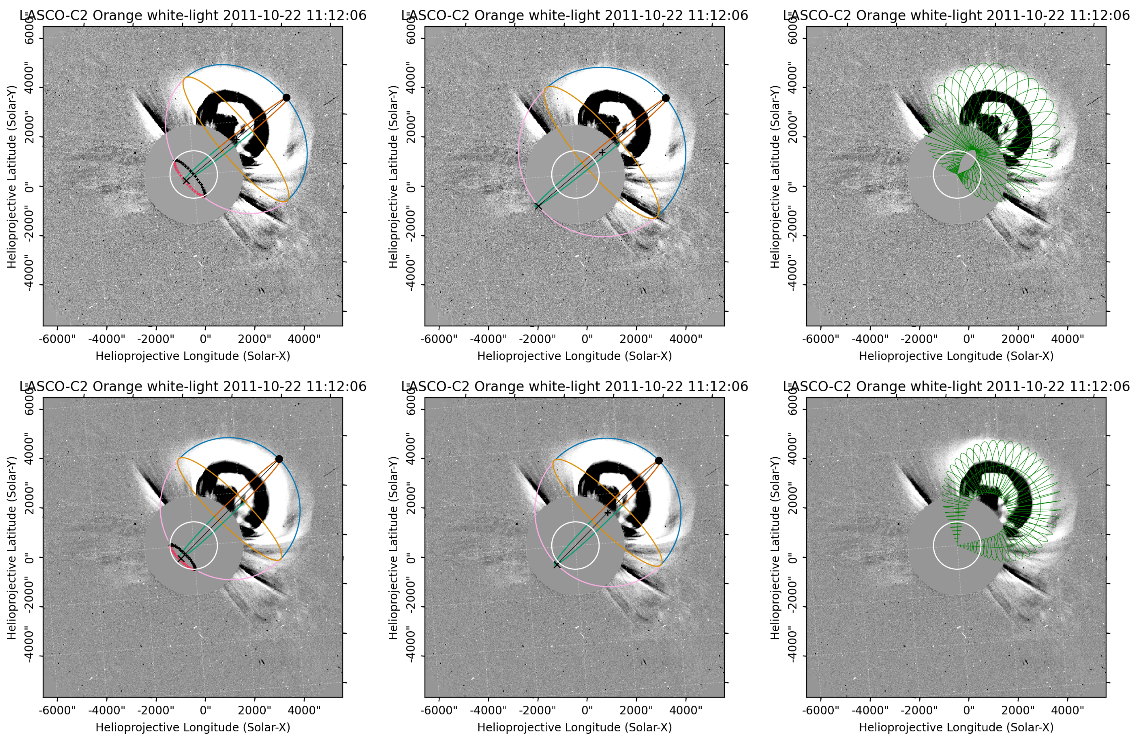
2.3. PyThea 3D De-Projection Tool

The de-projection technique used in this study is based on the novel PyThea online tool for 3D reconstruction of CMEs and shock waves [19]. All three models provided by PyThea are applied here: spheroid, ellipsoid and GCS. The fitting is completed by two observers from our team independently and an example of the fits for the event E03 is shown in Figure 1. Inspecting the fitting results for this example, we see that the reconstructions show a clear bias, as an observer has a subjective ’choice’ of structures to match with the model. Namely, in the top row of Figure 1 we observe clear shock-related structures (bending of streamers), which the idealized GCS flux rope geometry is fitted on. Hence, the CME width is most probably overestimated. We also find that the overall results, directivity and speed for this event (E03) are less affected by that bias. However, the more complex the choice of structures is, the larger the differences between several observers might be.

For this study we focused on deriving the de-projected CME speeds based on fits completed at two time steps. For each of the three models, the initial CME longitude and latitude was specified by hand. We used the provided locations of the CME-accompanied SFs. We note, however, that these values did not change (substantially or at all) after finalizing the fitting procedure; thus, the final CME directivity provided via PyThea is very crude. Thus, the final CME orientations in the IP space and at Earth are based only on the qualitative information provided by animations from the http://helioweather.net/archive/ (accessed on 24 February 2023).

3. Results

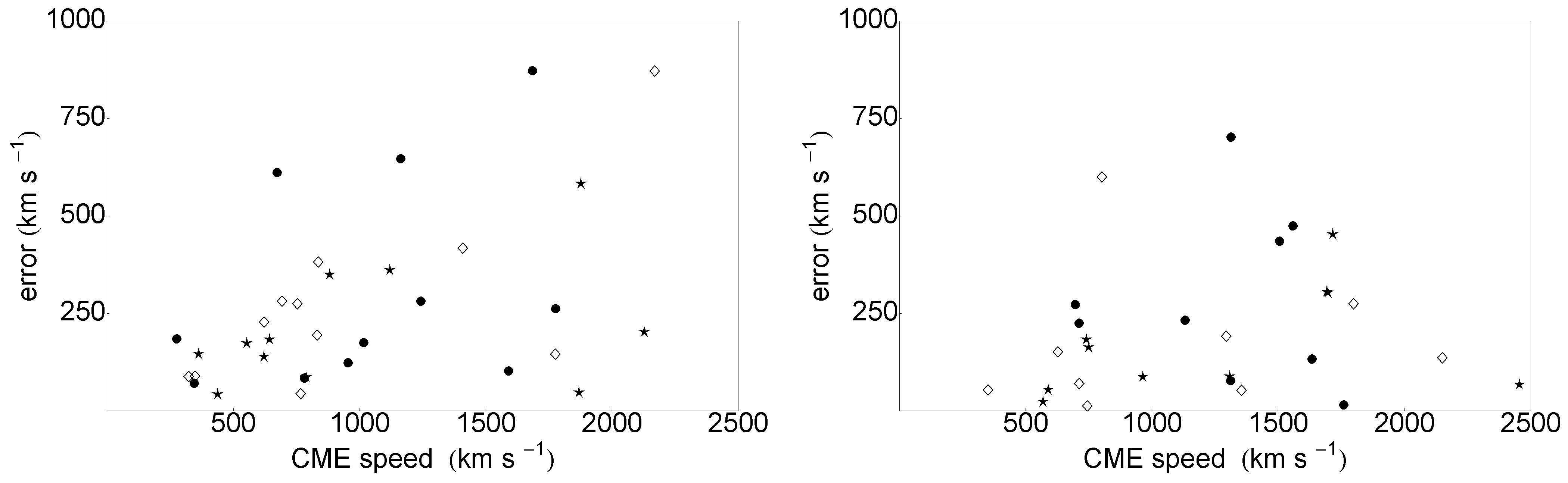
3.1. Projection Effects

Two observers from our team performed a fitting of about 10 CMEs using all three available models from the PyThea framework based on their own personal assessment. In summary, the fit is done at two time steps in order to deduce a speed based on the height–time estimation. For a given event, each observer repeated the 3D de-projection procedure twice and the averaged values for the CME speed are finally shown in

Table 3. Three-dimensional de-projected values of CME speed, in km s${}^{-1}$, averaged from the individual fits for observers (’obs’) 1 and 2. The event labels (in col. 1) are as in Table 1.

#	Spheroid		Ellipsoid		GCS
	obs1	obs2	obs1	obs2	obs1	obs2
E01	2170 ± 870	1800 ± 270	2130 ± 200	1710 ± 450	1590 ± 100	1760 ± 10
E02	1780 ± 140	1350 ± 50	1880 ± 580	1310 ± 90	1780 ± 260	1630 ± 130
E03	770 ± 40	740 ± 10	640 ± 180	740 ± 180	1020 ± 170	700 ± 270
E04	-	2150 ± 140	-	2460 ± 70	-	2530 ± 630
E06	1410 ± 420	710 ± 70	1870 ± 50	1700 ± 300	1680 ± 870	1560 ± 470
E08	350 ± 90	-	360 ± 150	-	350 ± 70	-
E09	690 ± 280	630 ± 150	550 ± 170	590 ± 60	670 ± 610	710 ± 220
E10	840 ± 380	610 ± 1040	1120 ± 360	960 ± 90	1160 ± 650	1310 ± 80
E13	320 ± 90	350 ± 50	620 ± 140	750 ± 160	780 ± 80	1310 ± 700
E20	830 ± 190	800 ± 600	790 ± 90	570 ± 20	1240 ± 280	1130 ± 230
E21	620 ± 230	-	440 ± 40	-	280 ± 180	-
E24	750 ± 270	1310 ± 220	880 ± 350	2020 ± 960	950 ± 120	1560 ± 540

(rounded to tenths). The offset between these two fits is given as an error (or uncertainty), ranging from 10 km s${}^{-1}$ to as large as twice the estimated speed. Furthermore, we plot the 3D speeds vs. the so-estimated errors in Figure 2 for each of the observers. Large scatters are evident in either plot, especially for the GCS model. Nevertheless, there is a rough positive trend between the value of the estimated error and the CME speed.

The individual subjectivity and level of experience of the observer are all inherent to such visual fitting procedure. Large differences in the evaluated speed can be seen not only between the individual observers for the same model (e.g., spheroid fit for E06), but also between different models by the same observer (e.g., spheroid and GCS for E13). Different operating system software was also used. E04, E08 and E21 could not be completed by both observers, either due to failure of the online PyThea computing resources or due to the large uncertainty of the visual assessment made on the CME structure. Overall, our results confirm the well known subjectivity that is part of any procedure which relies on a personal judgement of the quality of a fit, i.e., where structures would best match the model. This human-in-the-loop bias is explained in greater detail by [33]. The values of the CME speeds in detail can be seen in Table 3, whereas their average values, per model, between the two observers are listed in Table 2 and will be used for the correlation studies below.

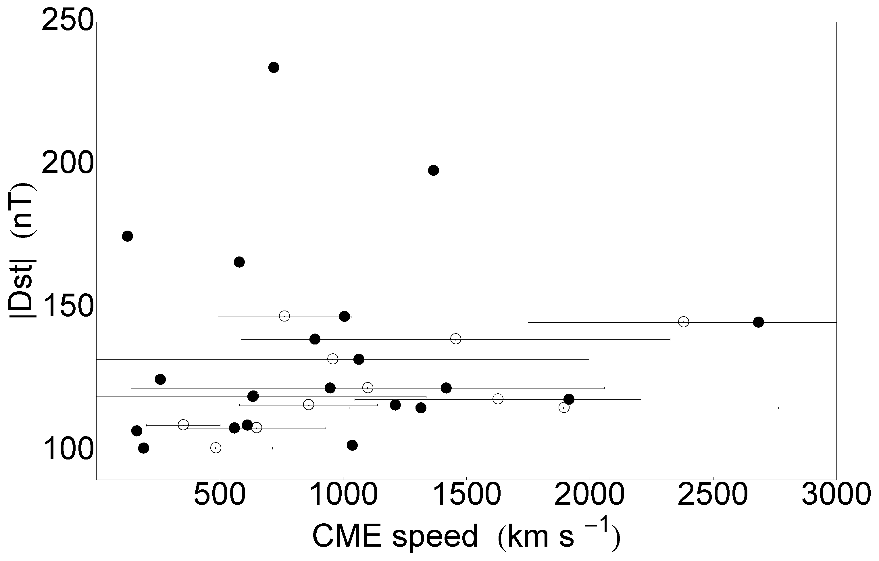
3.2. Correlation between GSs, Coronal and Near-Sun Parameters

The scatter-plot between the (modulus of the) GS Dst index and the CME speed (from Table 2) is presented in Figure 3. The results for each of the three model fits are again averaged (denoted as ’3D-mean’ in

Table 4. Table of Pearson correlation coefficients between GS Dst index, CME speed and other solar parameters. The sample size is given in parentheses.

CME Speed	Dst-CME Speed	Solar Parameter	Dst-Solar Parameter
LASCO	0.04 (20)	SF class	−0.04 (14)
3D-mean	0.49 (12)	SF latitude	−0.16 (14)
3D spheroid-mean	0.34 (12)	SF longitude	0.13 (14)
3D spheroid-obs1	0.14 (11)	CME AW	0.03 (20)
3D spheroid-obs2	0.15 (10)
3D ellipsoid-mean	0.53 (12)
3D ellipsoid-obs1	0.28 (11)
3D ellipsoid-obs2	0.40 (10)
3D GCS-mean	0.55 (12)
3D GCS-obs1	0.49 (11)
3D GCS-obs2	0.27 (10)

) and plotted there together with the 2D SOHO-LASCO CME speed. The error estimates of the 3D de-projections are also added for completeness, as horizontal lines, despite the large amount of overlap. The largest error value among the two observers (Table 3) is selected for demonstrative purposes.

The performed analysis indicates that no clear trend can be deduced between the Dst and the CME speed, also when using the 3D de-projection compared to the 2D CME speeds. Note that due to data issues, no 3D speed de-projections could be done for the strongest GSs. This is the reason for the shallow distribution of the 3D speeds, which skews the results. Despite the very small sample size (between 10 and 20 event pairs), we evaluate the goodness of the fit by means of Pearson correlations. The coefficients, between all CME speed estimations and the GS Dst index, are listed in Table 4 and range from no (e.g., 0.04 for the 2D LASCO speeds) to moderate correlations (with a maximum value of 0.55 based on the GCS model). There are no correlations between the Dst index and the other coronal parameters (SF class and location and CME AW), added for completeness in the same table.

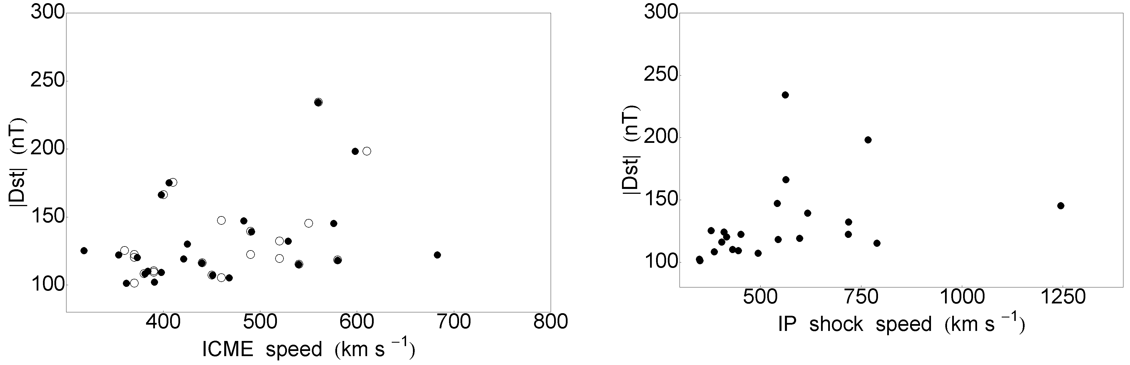
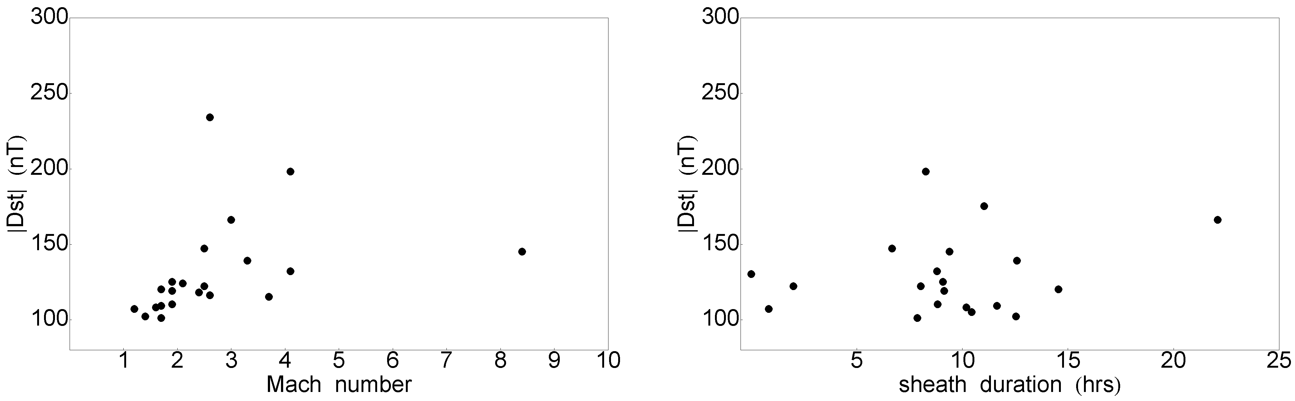
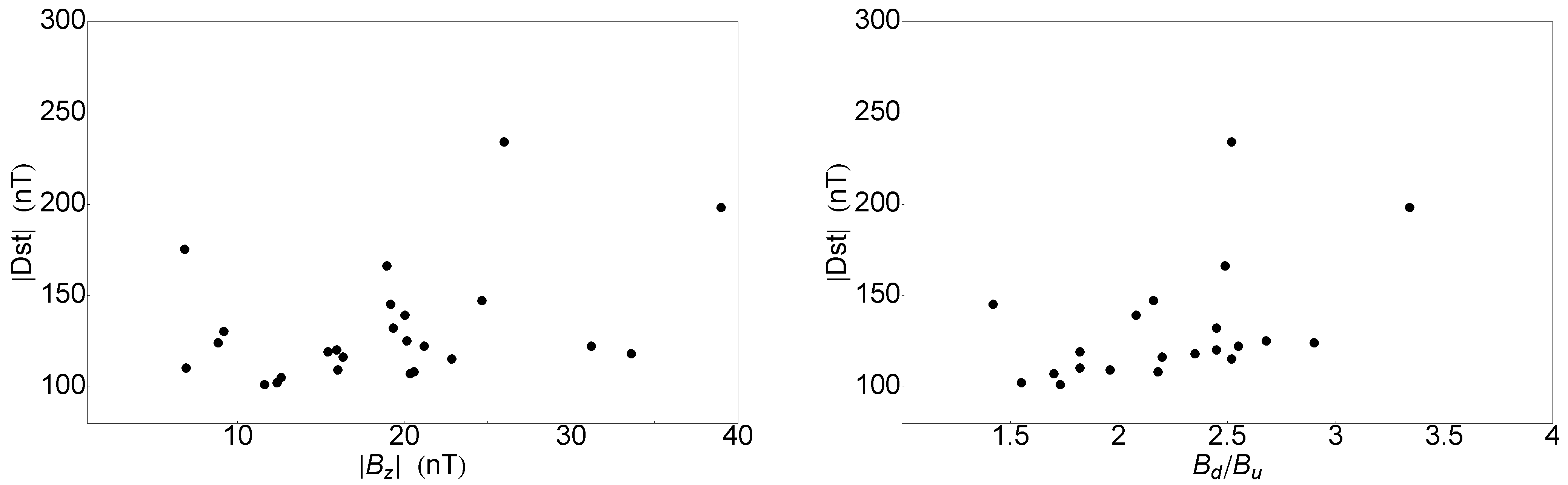
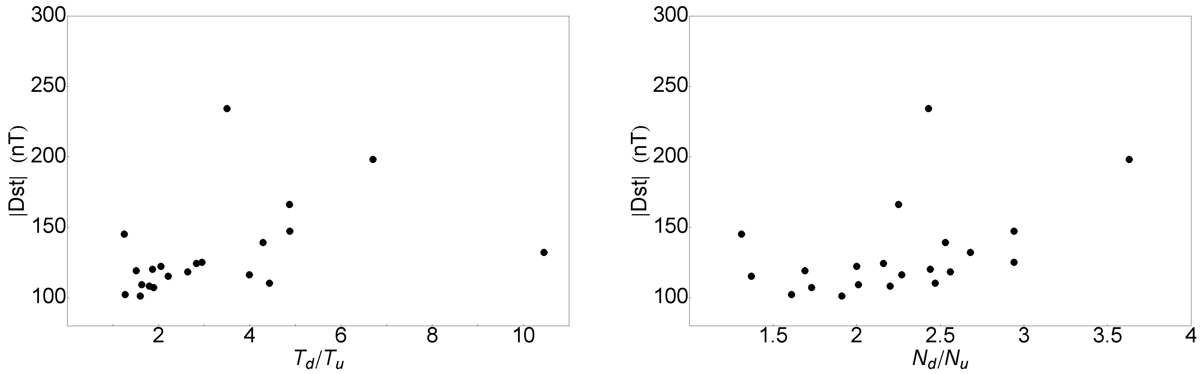
3.3. Correlation between GSs and IP Parameters

Here, we investigate the correlations between the GSs and the parameters of the pre-selected IP phenomena. Several pairs of parameters are explicitly visualized in scatter plots: the Dst index vs. ICME speed and IP shock speed in Figure 4; Dst vs. Mach number and sheath duration in Figure 5; Dst vs. $|B_z|$ and $B_d/B_u$ in Figure 6; and Dst vs. $T_d/T_u$ and $N_d/N_u$ in Figure 7. The numerical values of the correlation trends are given in

Table 5. Table of Pearson correlation coefficients between GS Dst index and different parameters of IP phenomena, based on Wind satellite data, unless specified explicitly. The sample size is given in parentheses.

IP Parameter	Dst-IP Parameter
ICME speed	0.37 (24)
ICME speed (ACE)	0.44 (22)
IP shock speed	0.35 (22)
Mach number	0.36 (21)
sheath duration	0.22 (20)
$|B_z|$	0.37 (25)
$B_d/B_u$	0.48 (21)
$T_d/T_u$	0.40 (21)
$N_d/N_u$	0.46 (21)
B	−0.14 (20)
V	0.19 (20)
${\beta }_u$	−0.14 (21)

in terms of Pearson correlations. For the small sample of GS storms used in our analyses, we obtain that the plasma compression parameters at the shock interface (downstream to upstream ratio) show a moderately positive trend with the Dst index. The Pearson correlations are similar to (or even slightly larger than) those obtained when ICME speeds (from Wind and ACE spacecraft) are used instead. Interestingly, the trend with the $|B_z|$ is weaker (0.37 for our list), despite the well known strong trend from previous studies. The calculated values between the Dst and IP shock speed, Mach number or the sheath duration are even smaller.

Strong correlations have been recently reported with different components of the electric and magnetic fields [12], which, however, goes beyond the scope of our analyses. Nevertheless, all these results should be applied with caution, since no uncertainty estimates of the correlation coefficients are calculated.

The used ICME and IP shock catalogs provide a number of additional parameters, e.g., averaged magnetic field B and plasma speed V inside the magnetic structure, upstream plasma beta ${\beta }_u$ (not shown in Table 1). No strong correlations are obtained between these parameters and the Dst index as all correlation coefficients found were smaller than 0.2.

3.4. On the GS Strength Forecasting Based on Solar and IP Parameters

We compare the combined effect between the magnetic obstacle type and orientation upon arrival at Earth (cols. 5 and 9 from Table 1) together with the 3D reconstructed CME speeds (cols. 10–12 from Table 2) on the GS strength (approximated in this study with the Dst index).

The strongest GSs in our list (listed in a descending order of their Dst, nT) have the following parameters of the magnetic structure in terms of complexity, orientation of arrival and speed at Earth (Table 1 and Table 2):

• E15 ($-234$): -, fast speed f, no 3D speed estimation
• E16 ($-198$): Cx, n, no 3D speed estimation
• E25 ($-175$): F+, n, no 3D speed estimation
• E19 ($-166$): Fr, n, no 3D speed estimation
• E03 ($-147$): Cx, f, reduced 3D speed compared to 2D
• E04 ($-145$): Cx, n, similar 3D speed compared to 2D
• E06 ($-139$): Fr, n, larger 3D speed compared to 2D
• E10 ($-132$): Fr, n, similar 3D speed compared to 2D

Upon inspection of the available cases, we conclude that the strongest GSs are due to magnetic obstacles with nose-like (n) orientation at arrival together with complex (Cx) or Fr (flux-rope) structure. The exceptions are either a fast speed flank hit or a flank hit in a combination of Cx structure. It was already shown that the sheath duration is not an ordering parameter. All remaining, weaker GSs (Table 1) are either flank hits or uncertain configurations (possibly due to fast solar wind streams or CIRs), apart from E20 which is due to a nose hit; however, the IP structure has a very low speed according to the inspected animations. We note that the IP shock speed provided by Wind and ACE satellite is in fact a single point sample out of the entire structure, whereas the animations tend to give the global speed distribution. Thus, for the interpretation here we consider the information provided by both sources, speed reconstructions and in situ measurements.

4. Discussion

In this study, we present post-event analyses of all GSs observed in SC24 in the search for distinct and reliable GS intensity predictors. The ultimate goal is to derive reliable solar or near-Sun parameters using remote sensing image data that can be applied for early warnings about potential GS onsets and strength. For that, we combined solar, near-Sun and IP parameters, mostly provided by catalogs but also analyzed by us using space-related databases. The results from the novel tool for CME speed de-projection (PyThea) are used for the first time together with the well known parameters in space weather and geophysics research.

From the considered solar and near-Sun phenomena, selected parameters show a positive correlation with the Dst index. In comparison to the observed projected CME speed, the correlation coefficient could be improved from 0.04 (LASCO) to 0.34–0.55 (using different geometrical models provided via PyThea software package combining LASCO and STEREO data). However, when applying the different CME geometry reconstruction techniques we reveal that especially fast CMEs seem to be prone to large speed errors. Similar results were derived in previous studies that focused on CME arrival time and speed forecasts for Earth, concluding that the CME launch speed might be overestimated for fast events [44]. This is most probably due to a higher complexity in the ’choice’ of coronal structures that become visible due to the larger compression related to the quickly expanding magnetic structure of the CME. Moreover, for fast halo CMEs large deviations might be found due to the overlap in shock and magnetic structure components strongly affecting the reconstruction quality. For that reason we conclude that the deduced near-Sun 3D parameters continue to have limited forecasting potential for forecasting the GS strength.

In comparison, most of the selected well known IP parameters deduced from in situ measurements show moderate positive correlations with the GS strength as expected [12]. However, for the $B_z$ parameter (i.e., the southward component of the magnetic field) we find a rather low correlation coefficient of 0.37. This could be due to the limited event sample used here. Other IP parameters, ICME and IP shock speeds, together with their derivative parameters (e.g., Mach number), show a positive trend with the Dst index and correlation coefficients of 0.35–0.45. Therefore, neither of these parameters can be considered as a prevailing one and moreover they are calculated based on single-point in situ observation. Comparing ACE and Wind measurements (see Figure 4) we derive differences in the ICME speed values. Slightly stronger correlation coefficients (0.4–0.5) are obtained when using different shock parameters, e.g., magnetic field, temperature and density jump at the shock profile. In contrast, averaged values of the magnetic field and speed in the magnetic structure, plasma beta in the upstream region or duration of the sheath region show no correlation with the GS strength.

Among all considered solar, near-Sun and IP parameters, only the combination of speed and orientation (nose-like) of the magnetic obstacle seem to have a positive feedback on the GS strength (Dst index), based on the qualitative results provided by http://helioweather.net/archive/ (accessed on 24 February 2023) animations. As concluded in previous studies, de-projected CME speeds are a necessity for improving the results when modeling CME propagation through the IP space [45]. However, there seems to be a lack of direct influence of the 3D de-projected CME speed on the GS intensity. Therefore, reliable estimation of the ICME speed distribution over the entire ICME structure upon arrival at Earth seems to be of great importance. Definitely, there is a clear need for permanent stereoscopic observations such as with future ESA Vigil mission that will be positioned at the Lagrange point L5. Future studies should seek a better disentanglement of different CME structures and hence more reliable 3D reconstructions of CME geometries to more reliably estimate the 3D speed and directivity.

References

1. Webb, D.F.; Howard, T.A. Coronal Mass Ejections: Observations. Living Rev. Sol. Phys. 2012, 9, 3. [Google Scholar] [CrossRef] [Green Version]
2. Fletcher, L.; Dennis, B.R.; Hudson, H.S.; Krucker, S.; Phillips, K.; Veronig, A.; Battaglia, M.; Bone, L.; Caspi, A.; Chen, Q.; et al. An Observational Overview of Solar Flares. Space Sci. Rev. 2011, 159, 19–106. [Google Scholar] [CrossRef] [Green Version]
3. Klein, K.L.; Dalla, S. Acceleration and Propagation of Solar Energetic Particles. Space Sci. Rev. 2017, 212, 1107–1136. [Google Scholar] [CrossRef]
4. Temmer, M. Space weather: The solar perspective. Living Rev. Sol. Phys. 2021, 18, 4. [Google Scholar] [CrossRef]
5. Malandraki, O.E.; Crosby, N.B. Solar Energetic Particles and Space Weather: Science and Applications. In Proceedings of the Solar Particle Radiation Storms Forecasting and Analysis; Malandraki, O.E., Crosby, N.B., Eds.; Astrophysics and Space Science Library; Springer Nature Publ.: Berlin/Heidelberg, Germany, 2018; Volume 444, pp. 1–26. [Google Scholar] [CrossRef] [Green Version]
6. Gopalswamy, N. The Sun and Space Weather. Atmosphere 2022, 13, 1781. [Google Scholar] [CrossRef]
7. Gonzalez, W.D.; Joselyn, J.A.; Kamide, Y.; Kroehl, H.W.; Rostoker, G.; Tsurutani, B.T.; Vasyliunas, V.M. What is a geomagnetic storm? J. Geophys. Res. 1994, 99, 5771–5792. [Google Scholar] [CrossRef] [Green Version]
8. Saiz, E.; Cerrato, Y.; Cid, C.; Dobrica, V.; Hejda, P.; Nenovski, P.; Stauning, P.; Bochnicek, J.; Danov, D.; Demetrescu, C.; et al. Geomagnetic response to solar and interplanetary disturbances. J. Space Weather. Space Clim. 2013, 3, A26. [Google Scholar] [CrossRef] [Green Version]
9. Lakhina, G.S.; Tsurutani, B.T. Geomagnetic storms: Historical perspective to modern view. Geosci. Lett. 2016, 3, 2196–4092. [Google Scholar] [CrossRef] [Green Version]
10. Dungey, J.W. The Steady State of the Chapman-Ferraro Problem in Two Dimensions. J. Geophys. Res. 1961, 66, 1043–1047. [Google Scholar] [CrossRef]
11. Akasofu, S.I. Energy coupling between the solar wind and the magnetosphere. Space Sci. Rev. 1981, 28, 121–190. [Google Scholar] [CrossRef]
12. Echer, E.; Gonzalez, W.D. Relation between Dst* and interplanetary parameters during single-step geomagnetic storms. Adv. Space Res. 2022, 70, 2830–2841. [Google Scholar] [CrossRef]
13. Tsurutani, B.T.; Gonzalez, W.D. The Interplanetary causes of magnetic storms: A review. Wash. DC Am. Geophys. Union Geophys. Monogr. Ser. 1997, 98, 77–89. [Google Scholar] [CrossRef]
14. Zhang, J.; Richardson, I.G.; Webb, D.F.; Gopalswamy, N.; Huttunen, E.; Kasper, J.C.; Nitta, N.V.; Poomvises, W.; Thompson, B.J.; Wu, C.C.; et al. Solar and interplanetary sources of major geomagnetic storms (Dst <= -100 nT) during 1996–2005. J. Geophys. Res. (Space Phys.) 2007, 112, A10102. [Google Scholar] [CrossRef] [Green Version]
15. Wu, C.C.; Lepping, R.P. Relationships Among Geomagnetic Storms, Interplanetary Shocks, Magnetic Clouds and Sunspot Number During 1995–2012. Solar Phys. 2016, 291, 265–284. [Google Scholar] [CrossRef]
16. Borovsky, J.E.; Denton, M.H. Differences between CME-driven storms and CIR-driven storms. J. Geophys. Res. (Space Phys.) 2006, 111, A07S08. [Google Scholar] [CrossRef] [Green Version]
17. Pulkkinen, T. Space Weather: Terrestrial Perspective. Living Rev. Sol. Phys. 2007, 4, 1. [Google Scholar] [CrossRef] [Green Version]
18. Paouris, E.; Vourlidas, A.; Papaioannou, A.; Anastasiadis, A. Assessing the Projection Correction of Coronal Mass Ejection Speeds on Time-of-Arrival Prediction Performance Using the Effective Acceleration Model. Space Weather. 2021, 19, e2020SW00261. [Google Scholar] [CrossRef]
19. Kouloumvakos, A.; Rodríguez-García, L.; Gieseler, J.; Price, D.J.; Vourlidas, A.; Vainio, R. PyThea: An open-source software package to perform 3D reconstruction of coronal mass ejections and shock waves. Front. Astron. Space Sci. 2022, 9, 974137. [Google Scholar] [CrossRef]
20. Samwel, S.W.; Miteva, R. Correlations between space weather parameters during intense geomagnetic storms: Analytical study. 2023; under review. [Google Scholar]
21. Kay, C.; Gopalswamy, N. The Effects of Uncertainty in Initial CME Input Parameters on Deflection, Rotation, Bz and Arrival Time Predictions. J. Geophys. Res. (Space Phys.) 2018, 123, 7220–7240. [Google Scholar] [CrossRef]
22. Vourlidas, A.; Wu, S.; Wang, A.; Subramanian, P.; Howard, R. Direct detection of a coronal mass ejection-associated shock in large angle and spectrometric coronagraph experiment white-light images. Astrophys. J. 2003, 598, 1392. [Google Scholar] [CrossRef]
23. Jackson, B.; Hick, P.; Buffington, A.; Bisi, M.; Clover, J.; Hamilton, M.; Tokumaru, M.; Fujiki, K. 3D Reconstruction of Density Enhancements Behind Interplanetary Shocks from Solar Mass Ejection Imager White-Light Observations. In Proceedings of the AIP Conference Proceedings. American Institute of Physics, Penang, Malaysia, 21–23 December 2010; Volume 1216, pp. 659–662. [Google Scholar]
24. Thernisien, A.; Vourlidas, A.; Howard, R.A. Forward Modeling of Coronal Mass Ejections Using STEREO/SECCHI Data. Solar Phys. 2009, 256, 111–130. [Google Scholar] [CrossRef]
25. Mierla, M.; Inhester, B.; Antunes, A.; Boursier, Y.; Byrne, J.P.; Colaninno, R.; Davila, J.; de Koning, C.A.; Gallagher, P.T.; Gissot, S.; et al. On the 3-D reconstruction of Coronal Mass Ejections using coronagraph data. Ann. Geophys. 2010, 28, 203–215. [Google Scholar] [CrossRef] [Green Version]
26. Wood, B.E.; Howard, R.A.; Socker, D.G. Reconstructing the Morphology of an Evolving Coronal Mass Ejection. Astrophys. J. 2010, 715, 1524–1532. [Google Scholar] [CrossRef] [Green Version]
27. Thernisien, A. Implementation of the Graduated Cylindrical Shell Model for the Three-dimensional Reconstruction of Coronal Mass Ejections. Astrophys. J. Suppl. 2011, 194, 33. [Google Scholar] [CrossRef]
28. Odstrcil, D.; Riley, P.; Zhao, X.P. Numerical simulation of the 12 May 1997 interplanetary CME event. J. Geophys. Res. (Space Phys.) 2004, 109, A02116. [Google Scholar] [CrossRef] [Green Version]
29. Xie, H.; Ofman, L.; Lawrence, G. Cone model for halo CMEs: Application to space weather forecasting. J. Geophys. Res. (Space Phys.) 2004, 109, A03109. [Google Scholar] [CrossRef]
30. Vršnak, B.; Žic, T.; Vrbanec, D.; Temmer, M.; Rollett, T.; Möstl, C.; Veronig, A.; Čalogović, J.; Dumbović, M.; Lulić, S.; et al. Propagation of Interplanetary Coronal Mass Ejections: The Drag-Based Model. Solar Phys. 2013, 285, 295–315. [Google Scholar] [CrossRef]
31. Pomoell, J.; Poedts, S. EUHFORIA: European heliospheric forecasting information asset. J. Space Weather. Space Clim. 2018, 8, A35. [Google Scholar] [CrossRef] [Green Version]
32. Jang, S.; Moon, Y.J.; Kim, R.S.; Lee, H.; Cho, K.S. Comparison between 2D and 3D Parameters of 306 Front-side Halo CMEs from 2009 to 2013. Astrophys. J. 2016, 821, 95. [Google Scholar] [CrossRef] [Green Version]
33. Verbeke, C.; Mays, M.L.; Kay, C.; Riley, P.; Palmerio, E.; Dumbović, M.; Mierla, M.; Scolini, C.; Temmer, M.; Paouris, E.; et al. Quantifying errors in 3D CME parameters derived from synthetic data using white-light reconstruction techniques. Adv. Space Res. 2022, (in press). [Google Scholar] [CrossRef]
34. Gopalswamy, N.; Yashiro, S.; Akiyama, S.; Xie, H.; Mäkelä, P.; Fok, M.C.; Ferradas, C.P. What Is Unusual About the Third Largest Geomagnetic Storm of Solar Cycle 24? J. Geophys. Res. (Space Phys.) 2022, 127, e30404. [Google Scholar] [CrossRef]
35. Qiu, S.; Zhang, Z.; Yousof, H.; Soon, W.; Jia, M.; Tang, W.; Dou, X. The interplanetary origins of geomagnetic storm with Dstmin ≤ - 50 nT during solar cycle 24 (2009–2019). Adv. Space Res. 2022, 70, 2047–2057. [Google Scholar] [CrossRef]
36. Besliu-Ionescu, D.; Maris Muntean, G.; Dobrica, V. Complex Catalogue of High Speed Streams Associated with Geomagnetic Storms during Solar Cycle 24. Solar Phys. 2022, 297, 65. [Google Scholar] [CrossRef]
37. Abe, O.E.; Fakomiti, M.O.; Igboama, W.N.; Akinola, O.O.; Ogunmodimu, O.; Migoya-Orué, Y.O. Statistical analysis of the occurrence rate of geomagnetic storms during solar cycles 20–24. Adv. Space Res. 2023, 71, 2240–2251. [Google Scholar] [CrossRef]
38. Selvakumaran, R.; Veenadhari, B.; Akiyama, S.; Pandya, M.; Gopalswamy, N.; Yashiro, S.; Kumar, S.; Mäkelä, P.; Xie, H. On the reduced geoeffectiveness of solar cycle 24: A moderate storm perspective. J. Geophys. Res. (Space Phys.) 2016, 121, 8188–8202. [Google Scholar] [CrossRef]
39. Gonzalez, W.D.; Echer, E.; Clua-Gonzalez, A.L.; Tsurutani, B.T. Interplanetary origin of intense geomagnetic storms (Dst < -100 nT) during solar cycle 23. Geophys. Res. Lett. 2007, 34, L06101. [Google Scholar] [CrossRef] [Green Version]
40. Gopalswamy, N.; Akiyama, S.; Yashiro, S.; Michalek, G.; Lepping, R.P. Solar sources and geospace consequences of interplanetary magnetic clouds observed during solar cycle 23. J. Atmos.-Sol.-Terr. Phys. 2008, 70, 245–253. [Google Scholar] [CrossRef]
41. Echer, E.; Tsurutani, B.T.; Gonzalez, W.D. Interplanetary origins of moderate (−100 nT < Dst ≤ −50 nT) geomagnetic storms during solar cycle 23 (1996–2008). J. Geophys. Res. (Space Phys.) 2013, 118, 385–392. [Google Scholar] [CrossRef] [Green Version]
42. Manu, V.; Balan, N.; Zhang, Q.H.; Xing, Z.Y. Association of the Main Phase of the Geomagnetic Storms in Solar Cycles 23 and 24 with Corresponding Solar Wind-IMF Parameters. J. Geophys. Res. (Space Phys.) 2022, 127, e2022JA030747. [Google Scholar] [CrossRef]
43. Nieves-Chinchilla, T.; Vourlidas, A.; Raymond, J.C.; Linton, M.G.; Al-haddad, N.; Savani, N.P.; Szabo, A.; Hidalgo, M.A. Understanding the Internal Magnetic Field Configurations of ICMEs Using More than 20 Years of Wind Observations. Solar Phys. 2018, 293, 25. [Google Scholar] [CrossRef]
44. Dumbović, M.; Čalogović, J.; Vršnak, B.; Temmer, M.; Mays, M.L.; Veronig, A.; Piantschitsch, I. The Drag-based Ensemble Model (DBEM) for Coronal Mass Ejection Propagation. Astrophys. J. 2018, 854, 180. [Google Scholar] [CrossRef]
45. Mays, M.L.; Thompson, B.J.; Jian, L.K.; Colaninno, R.C.; Odstrcil, D.; Möstl, C.; Temmer, M.; Savani, N.P.; Collinson, G.; Taktakishvili, A.; et al. Propagation of the 7 January 2014 CME and Resulting Geomagnetic Non-event. Astrophys. J. 2015, 812, 145. [Google Scholar] [CrossRef] [Green Version]
Figure 1. Three-dimensional reconstructions of a CME (E03) using the spheroid (left), ellipsoid (middle) and GCS model (right column) from the PyThea tool performed by observers 1 and 2 (top and bottom rows, respectively).
Universe 09 00179 g001
Figure 2. Scatter-plot between the 3D de-projection CME speeds obtained from the spheroid model (diamonds), the ellipsoid model (stars) and the GCS model (dots) and the error of the measurements for observers 1 (left) and 2 (right plot).
Universe 09 00179 g002
Figure 3. Scatter plot between the Dst index and CME speed: from the SOHO/LASCO instrument (with filled circles) and from the 3D de-projections (with empty circles).
Universe 09 00179 g003
Figure 4. Scatter plots between Dst index and Wind/ACE ICME speed (left, filled/empty symbols) and IP shock speed (right).
Universe 09 00179 g004
Figure 5. Scatter plots between Dst index and Mach number (left) and duration of sheath region (right).
Universe 09 00179 g005
Figure 6. Scatter plots between Dst index and Bz (left) and magnetic field jump (right).
Universe 09 00179 g006
Figure 7. Scatter plots between Dst index and temperature jump (left) and density jump (right).
Universe 09 00179 g007