Article

Temperature Variations in the Mesosphere and Lower Thermosphere during Geomagnetic Storms with Disparate Durations at High Latitudes

1
Institute of Space Weather, School of Atmospheric Physics, Nanjing University of Information Science & Technology, Nanjing 210044, China
2
High Altitude Observatory, National Center for Atmospheric Research, Boulder, CO 80307, USA
3
Kunming General Survey of Natural Resources Center, China Geological Survey, Kunming 650108, China
4
Institute of Energy and Climate Research, IEK-7: Stratosphere, Forschungszentrum Jülich, 52425 Jülich, Germany
*
Author to whom correspondence should be addressed.
Universe 2023, 9(2), 86; https://doi.org/10.3390/universe9020086
Submission received: 6 December 2022 / Revised: 18 January 2023 / Accepted: 2 February 2023 / Published: 5 February 2023
(This article belongs to the Special Issue Auroral Physics)

Abstract

:
Using the temperature data observed from the Sounding of the Atmosphere using Broadband Emission Radiometry (SABER), we investigate the response of the mesosphere and lower thermosphere (MLT) to two medium geomagnetic storms with disparate durations, on 20 April 2018 and 10 April 2022. The high-latitude MLT temperature increase in the Southern hemisphere can reach 40 K during April 2018 geomagnetic storm with a longer duration (Kp values greater than 4 for 15 h), while the temperature variations are less than 10 K for the April 2022 event (Kp values greater than 4 for 6 h). To investigate the different temperature responses to disparate geomagnetic storm durations and understand what physical process results in this difference, we simulated the two events using the thermosphere ionosphere mesosphere electrodynamics general circulation model (TIMEGCM). The simulations show that more particles and energy input in longer-duration geomagnetic storms produce larger ion drag force and pressure gradient force at ~130 km, and then the enhanced two forces cause faster horizontal wind, leading to larger horizontal divergence. Subsequently, the stronger downward vertical wind is transported to the MLT region (below 110 km) and ultimately makes greater temperature increases through adiabatic heating/cooling and vertical advection. Therefore, the effects of the storm’s duration on the MLT temperature are also important.

1. Introduction

During a geomagnetic storm, charged particles and electromagnetic energy are injected into the Earth’s atmosphere at high latitudes due to solar wind–magnetosphere–ionosphere coupling, leading to kinetic temperature changes in the mesosphere and lower thermosphere (MLT) region through complex physical and chemical processes, such as Joule heating and infrared radiative cooling [1,2,3]. The storm-time perturbation of the temperature in the MLT region was reported and explained by many studies. Von Savigny et al. [4] found a temperature increase of ~15 K near 85 km in the polar region during the January 2005 geomagnetic storm accompanied by a solar proton event. They speculated that this increase in temperature was caused by the precipitating protons. Pancheva et al. [5] showed that the temperature significantly decreased with an amplitude of 25 K at ~90 km during the geomagnetic storm in late October 2003, which they attributed to the reduction in ozone. Nesse Tyssøy et al. [6] analyzed Na radar temperature data during an intense geomagnetic storm in January 2005 and found that the temperature above 90 km was higher than the monthly average. They concluded that the processes were associated with particle precipitation and Joule heating. Fang et al. [7] and Xu et al. [8] showed that polar heating could penetrate down to 105 km during geomagnetic storms at high latitudes. Yuan et al. [9] studied four geomagnetic storm events, using the temperature/wind Doppler Na lidar, and found a significant temperature increase above 95 km in the middle latitudes. The temperature increases were more than 55 K above 105 km. They suggested that the temperature increase is closely related to the decrease in O/N2. Geomagnetic activity not only affects the wind field in the thermosphere [10,11], but also the wind in the MLT region, which leads to temperature variations. Using the temperature data measured by the sounding of the atmosphere using broadband emission radiometry (SABER) instrument onboard the thermosphere, ionosphere, mesosphere energetics, and dynamics (TIMED) satellite, Liu et al. [12] analyzed the geomagnetic storm in March 2013. They found that the temperature increase was more than 30 K at 80° S around 110 km. They concluded that the global temperature perturbation in the MLT region is caused by global circulation changes associated with heating and ion drag in the auroral region. The simulation results of Li et al. [13,14] show that the warming above 105 km during magnetic storms could exceed 30 K at 60° N. They demonstrated that the mid-latitude temperature variations are mainly caused by adiabatic heating/cooling and vertical transport using TIMEGCM thermodynamic diagnostic analysis during storms in the MLT region. Both heating/cooling terms are associated with vertical wind perturbations due to atmospheric circulation changes. A recent statistical study of SABER data showed about a 4 K temperature increase at the mesopause around 95 km, with a response delay of up to 1 day during strong geomagnetic activity from 2002 to 2018 [15]. Recently, Sun et al. [16] found that the TIMED/SABER temperature increase was greater than ~35 K above 100 km at 80° N in a geomagnetic storm on 7 September 2017. They suggested that vertical winds play a vital role in the warming process. These studies also explored the causes of temperature variations by latitude and found that they are dominated by Joule heating and particle precipitation at high latitudes, and by dynamic and chemical processes in the middle latitudes. In addition, MLT temperature response to different sources of geomagnetic activity varies. Using SABER observations, Wang et al. [3] showed that the temperature enhancement penetrated deeper in CME-induced geomagnetic activities, while the temperature increase lasted longer in CIR-induced geomagnetic activities.
Previous studies focused on the temperature change finding in the MLT region during magnetic storms, physical mechanisms exploration, and analysis of the temperature response under different kinds of magnetic storms. However, the effects of differences in the duration of geomagnetic disturbances on the MLT temperature changes were not clear.
Kp index is an index used to measure global magnetic disturbances, which ranges from 0 to 9. Two medium geomagnetic storms occurred on 20 April 2018 and 10 April 2022, in the same season but with disparate durations of large Kp values. The 2018 storm had a maximum Kp value of 6, and the Kp value greater than 4 lasted for 15 h. In contrast, the 2022 event had a maximum Kp value of 7, and the disturbance is a bit stronger than that in the 2018 event. The Kp values greater than 4 lasted only 6 h in the 2022 event, which is far shorter by comparison. These two storms in 2018 (weaker but longer duration) and 2022 (stronger but shorter duration) are studied to discuss the differences in the MLT temperature variations during storms with disparate durations of large Kp values using temperature observations from SABER and simulations from TIMEGCM (driven by 3 h Kp index).

2. Data and Method

2.1. SABER

SABER is the instrument on board the TIMED satellite. Its main mission is to provide kinetic temperature, density, infrared radiative rate, and atmospheric composition to improve the understanding of the fundamental processes controlling the energy, chemistry, dynamics, and transport in the MLT region [17,18,19]. We selected two geomagnetic storm events with similar Kp values on 10 April 2018 and 22 April 2022, respectively. The SABER neutral temperature profiles (V2.07, Level 2A) from 80 km to 110 km were used to study the impacts of these storms on the MLT region. The latitude coverage of satellite observations shifts between 53° N and 83° S (south viewing mode) and 83° N and 53° S (north viewing mode) every 60 days. In this work, the TIMED/SABER instrument viewed from approximately 53° N to 83° S.

2.2. TIMEGCM

The TIMEGCM is a self-consistent global numerical atmospheric model developed by the National Center of Atmosphere Research (NCAR) [20,21], which calculates the continuity, momentum, and energy equations to simulate physical and chemical processes. The heights of the lower and upper boundaries of the model are ~30 km and ~600 km, respectively, while the horizontal resolution of the TIMEGCM is 2.5° by 2.5° and the vertical resolution is 1/4 scale height. The convective electric field applied at high latitudes is obtained from the Heelis model driven by the 3 h Kp index [22].
The TIMEGCM calculates the variations of neutral temperature by solving the thermodynamic equation:
T n t = g e z p 0 C p Z K T H T n Z + K E H 2 C p ρ g C p + 1 H T Z v n · T n W n T n Z + R T n C p m ¯ + Q L C p
where T n is the neutral temperature, t is the time, g is the gravitational acceleration, p 0 is the reference pressure, C p is the specific heat per unit mass for constant pressure, K T is the molecular thermal conductivity, H is the pressure scale height, K E is the eddy diffusion coefficient, ρ is the atmospheric mass density, v n is the horizontal wind velocity, W n is the vertical wind speed, R is the universal gas constant, and m ¯ is the mean molecular mass, respectively. The heating and cooling terms on the right side of the equation determine the neutral temperature changes. They are heat transfer by vertical molecular heat conduction ( g e z p 0 C p Z K T H T n Z ), eddy diffusion ( g e z p 0 C p Z K E H 2 C p ρ g C p + 1 H T Z ), horizontal advection ( v n · T n ), vertical heat advection ( W n T n Z ), adiabatic heating/cooling ( W n R T n C p m ¯ ), and other heating and cooling processes ( Q and L ), such as Joule heating and infrared radiation cooling. This equation gives the contribution of each heating/cooling term to the temperature variation, allowing us to quantify the effects of each process, which is known as thermodynamic diagnostic analysis.
The formula for calculating the vertical wind in TIMEGCM is shown in the equation:
W n z = e 1 2 z e 1 2 z W n z Δ z + Δ z H · v n z
where W n is the vertical wind speed, z is the scale height, W n z Δ z is the vertical wind speed at an upper level, H · v n is the horizontal wind divergence, and the expression is:
H · v n = 1 R E cos λ U n ϕ + V n cos λ λ
where R E is the radius of the Earth, λ is the latitude, Φ is the longitude, U n is the zonal wind speed, and V n is the meridional wind speed, respectively. According to formulas 2 and 3, dynamic diagnostic analysis can be carried out to analyze the cause of vertical wind disturbance.
The meridional and zonal momentum equations are defined as:
V n t = g e z p 0 Z μ V n H Z f c o r U n + λ y y V i V n + λ y x U i U n v n · V n + U n U n R E tan λ 1 R E Φ λ W n V n Z
U n t = g e z p 0 Z μ U n H Z + f c o r V n + λ x x V i V n + λ x y U i U n v n · U n + U n V n R E tan λ 1 R E cos λ Φ ϕ W n U n Z
where t is time, λ is latitude, ϕ is longitude, g is gravitational acceleration, p 0 is reference pressure, μ is viscosity coefficients, H is pressure scale height, f c o r is the Coriolis parameter, λ y x and λ y y are ion drag coefficients, V n and V i are neutral and ion meridional speeds, U n and U i are neutral and ion zonal speeds, v n is the horizontal wind velocity, R E is Earth radius, Φ is pressure, and W n is the vertical wind speed, respectively. The terms (meridional) on the right side are the vertical viscosity ( g e z p 0 Z μ V n H Z ), Coriolis force ( f c o r U n ), ion drag force ( λ y y V i V n + λ y x U i U n ), horizontal advection ( v n · V n ), centrifugal force ( U n U n R E tan λ ), pressure gradient force ( 1 R E Φ λ ), and vertical advection ( W n V n Z ), respectively. The zonal terms are similar to those of meridional terms. By comparing the contribution of each heating term in Equations (4) and (5), the cause of horizontal wind field changes can be explained, which are called kinetic diagnostic analysis.

2.3. Experimental Method

First, simulations with geomagnetic storm effects were obtained using the real Kp value of both events as the driving condition (rkp for short). After that, the Kp values for the day of the magnetic storms were set to a constant value to obtain simulations without storm effects (ckp for short). Based on the mean Kp values for the two days before the geomagnetic storm, the constant Kp value was set to 1 on 20 April 2018, and 2+ on 10 April 2022. The differences between the simulations driven by different geophysical conditions (rkp−ckp) eliminate the effects of factors such as tidal waves and represent the effects caused by geomagnetic storms. Afterward, the differences and causes of temperature variations in high-latitude MLT regions during geomagnetic storms with different durations were revealed by thermodynamic diagnostic analysis. On this basis, the difference in the vertical wind was caused by the difference between vertical wind in the upper layer and horizontal divergence in the same layer. Then, the horizontal divergence term breaks into zonal component and meridional component, and the zonal wind and meridional wind were used to explain the differences between the two storms. Finally, the physical mechanism of the difference in the horizontal wind was explained by kinetic diagnostic analysis.

3. Results

A geomagnetic storm with a short duration of large Kp values occurred on 10 April 2022. To study the effect of the duration of storms on MLT temperature, we compared a similar geomagnetic storm on 20 April 2018. In the 2018 storm, the main phases started at 00:28 UT on 20 April; after that, the recovery phase started at 09:35 UT [23]. The blue lines in Figure 1 give the Kp values during the storms, where the Kp maximum for the 2018 storm event was 6, occurring at 09:00 UT on 20 April. The Kp maximum for the 2022 storm was 7, occurring at 06:00 UT on 10 April. The first row of Figure 1 shows the SABER temperature variations in the range of 80 km to 110 km at high latitudes (from 77.5° S to 82.5° S) for both events. The zonal running mean was used to remove the effects of tides and small-scale waves [10,24,25,26]. After that, the temperature changes caused by the storms were calculated by subtracting the mean temperature of the two days before the storms. The results show that the temperature increases can reach a maximum value of ~40 K in the MLT region on 21 April 2018. However, the maximum increase in neutral temperature was just about 10 K during the geomagnetic storm on 11 April 2022, in the altitude range of 80 km to 110 km. In addition, both two events showed similar cooling above 100 km from the onset of the geomagnetic storms.
To study the differences between the two storms, we simulated the two geomagnetic storms using the TIMEGCM and obtained the temperature simulations at the satellite location. The same zonal running mean was processed. Then, the average simulated temperature of the two days before the start of the storms was subtracted from simulations driven by the true geophysical conditions. The simulations (same as the first row of Figure 1) are shown in the second row of Figure 1. It shows that the simulations for the two storms agree well with the SABER observations. In the 2018 storm, cooling was observed from 95 km to 110 km at the beginning of the magnetic storm. After that, the simulations also showed temperature increases from 10:00 UT on the 20th. The increases penetrated down to 100 km and reached a maximum of 40 K at 110 km at 06:00 UT on the 21st. In addition, the simulations for April 2022 also showed a temperature decrease after the start of the geomagnetic storm, which reached −7 K at 12:00 UT on the 10th. Afterward, near the end of 10 April, the temperature increase occurred at 110 km, which reached 9 K at 02:00 UT on the 11th and went down to 106 km.
It was noted that the influence of some additional factors, such as local time, F10.7, and so on, between the storms and quiet time cannot be eliminated in the first and second rows of Figure 1. To remove the effects of other factors, temperature changes were calculated by subtracting the simulated data driven by non-disturbed geophysical conditions (ckp) from the simulated data driven by the true geophysical conditions (rkp), which are shown in the third row of Figure 1. The results are similar to those in the first and second rows. The simulations for the 2018 storm first showed cooling above 100 km on 20 April (day 110), which propagated downward over time to 95 km with a minimum of −6 K. The temperature increases initially occurred at 110 km at 10:00 UT on the 20th. The temperature increases can reach 45 K at 110 km and propagate downward to ~98 km over time. In contrast, the simulations for the 2022 storm with a shorter duration were more different. The cooling in the early phase of the 2022 storm was more pronounced, nearly 8 K. Then, the temperature increased less than 10 K in the recovery phase, only dipping to ~102 km. Therefore, the duration of a geomagnetic storm has a significant impact on the magnitude and height of the temperature variation in the MLT region.
Figure 2 shows the southern hemispheric variations of temperature (rkp−ckp) at 110 km for the two storms at high latitudes. The locations of the satellite observation points at the corresponding time were marked with black asterisks in Figure 2. During the initial phase of the storms (the first row in Figure 2, 01:00 UT on the first day of the two geomagnetic storms), the temperature of the two storms did not change significantly. The temperature variations at 12:00 UT on the first day of the two storms, corresponding to the main phase, are shown in the second row. The temperature changes between the two storms were very similar, which showed a minimum temperature region near the poles and two maximum temperature regions near 120° E and 165° W. The decreased temperature minimum for the 2018 storm was −53 K, compared to −42 K and a smaller region for the 2022 storm. Meanwhile, the maximum temperature increase for the 2022 storm was 48 K, which was a great deal weaker than the 75 K for the 2018 storm. At 18:00 UT on the first day of the storms and during the recovery phase, significant temperature variations occurred between the two storms. In the 2018 storm, the region of the minimum temperature appeared near 107° W and 65° S, where the temperature decreases were less than 5 K. There were two maximum temperature regions at the same time. The maximum temperature region at high latitudes was located near 40° E and 70° S, and the increased maximum was more than 100 K. However, the temperature increases of the April 2022 geomagnetic storm were relatively small, and its increased maximum was only about 40 K. At 12:00 UT on the second day of the geomagnetic storm (fourth row in Figure 2), the temperature increases during the 2018 geomagnetic storm were still above 50 K, but those of the 2022 storm are already less than 20 K and will end soon. The position of (78.75° S, 60° E), the green dot in Figure 2, was selected as the reference point for analyzing the physical processes causing the differences in temperature variations between the two storms because it was close to the area with the maximum temperature increases in both events compared with other points at the same latitude.

4. Discussion

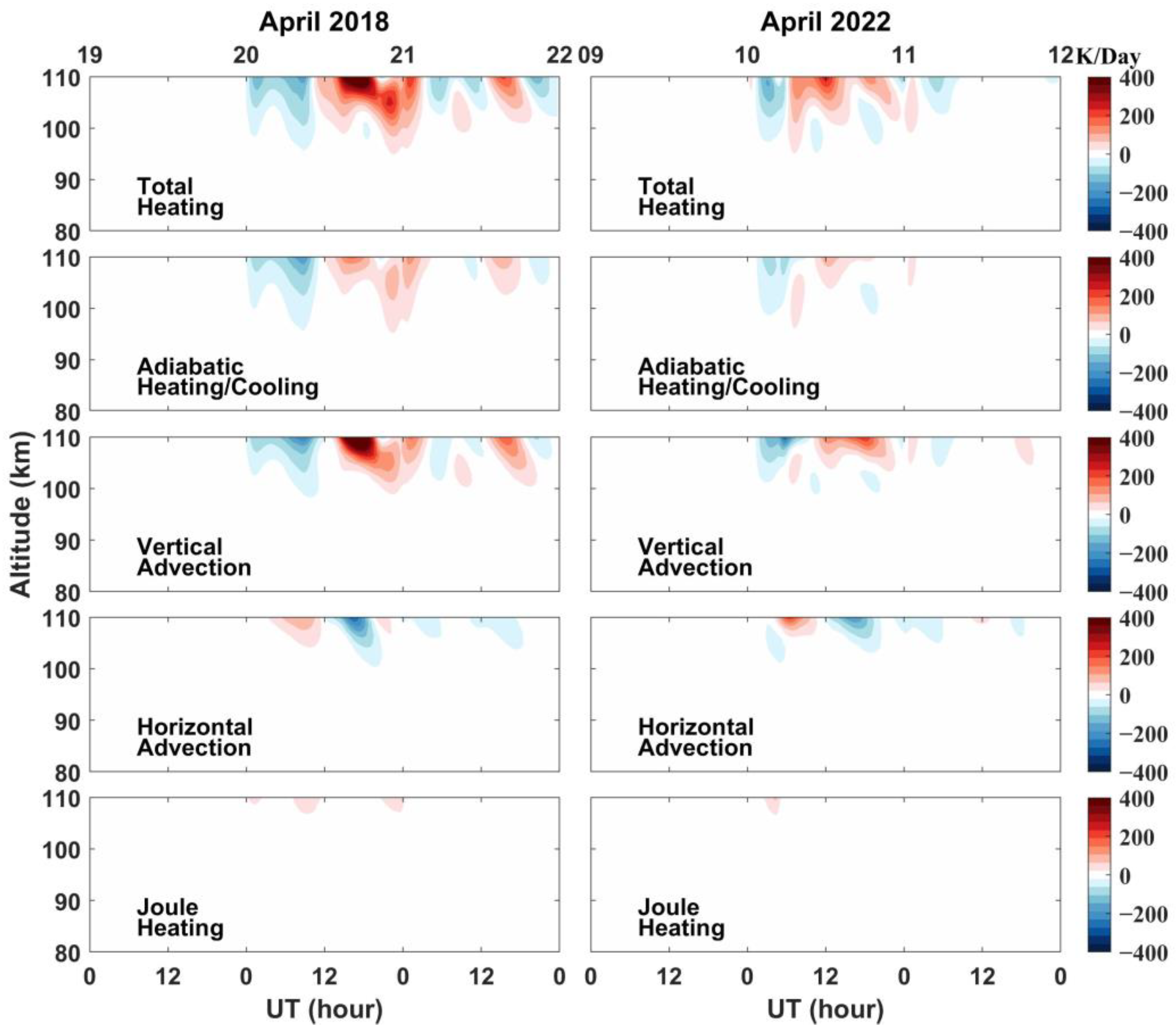
The results of the thermodynamic diagnostic analysis from 80 km to 110 km at (78.75° S, 60° E) were shown in Figure 3. The first row showed the difference in the total heating (rkp−ckp) and the following four rows showed the difference in the four main heating terms. The rest of the heating terms (not shown) were minor for the total heating. A cooling occurred and lasted for nearly 10 h at the beginning of the April 2018 storm, which reached −150 K/day at 110 km. The subsequent heating from 10:00 UT on the 20th to 03:00 UT on the 21st was mainly caused by vertical advection and adiabatic heating. The total heating at 110 km reached a maximum of ~530 K/day at 17:40 UT on the 20th, when the contributions of adiabatic heating, vertical advection, and horizontal advection were ~140 K/day, ~620 K/day, and ~−190 K/day, respectively. The beginning of the April 2022 storm also showed a cooling of −150 K/day, but its duration was only half that of the 2018 storm. The subsequent heating had the same duration as the 2022 storm, but was considerably weaker, with a maximum of only ~260 K/day at 12:00 UT on the 10th. The main contributors to the total heating were also vertical advection (150 K/day) and adiabatic heating (90 K/day). The contribution of the horizontal advection to the temperature increases in both storms was essentially negative after 12:00 UT on the first day of the storms. The position was adjacent to the maximum temperature region. As a result, the pressure gradient drove winds outward, and cooling appeared. Similarly, the contribution of Joule heating to the total heating was minor due to the position being located in the polar cap. Therefore, the temperature increases at the position (78.75° S, 60° E) in both events were mainly caused by adiabatic heating and vertical advection, both of which were caused by downward vertical winds. The density of the thermosphere decreases and the temperature increases with increasing altitudes. The downward vertical wind brought the less dense and warmer atmosphere from the upper pressure level to the lower pressure level, which increased the temperature of the lower pressure level through adiabatic compression and heat conduction.
The vertical wind is determined by the vertical term ( e 1 2 z e 1 2 z W n z Δ z ) reflecting the upper vertical wind and the horizontal term ( e 1 2 z Δ z H · v n ) reflecting the divergence of horizontal wind at the same pressure level, as shown in Equation 2. To investigate the origin of the vertical wind that caused adiabatic heating and vertical advection as described above, the diagnostic analysis of the vertical wind from 90 km to 150 km at the same position (78.75° S, 60° E) is given in Figure 4. The first row shows the vertical wind difference, and the following two rows show the contributions of the vertical winds and the divergence of horizontal winds, respectively. In the 2018 storm, the upward vertical winds first appeared, with a maximum of 20 cm/s at 110 km. This corresponded to the cooling caused by adiabatic heating/cooling and vertical convection at the beginning of the storm in Figure 3, which directly caused the temperature decreases at 12:00 UT (green dot in the second row of Figure 2) on the first day of the storm. Subsequently, the originally upward vertical winds at 110 km turned downward at 11:20 UT. The diagnostic analysis of the vertical wind showed that the change in the horizontal winds below 150 km first caused horizontal convergence, which weakened the upward vertical winds and eventually changed the vertical wind direction. The downward vertical winds occurred below 140 km. The contribution of the convergence term to the downward vertical winds reached a maximum of 35 cm/s around 125 km at 15:40 UT on the 20th, which greatly strengthened the downward vertical wind at that height. Afterward, the vertical winds were transported to the lower altitudes according to the vertical term (second row in Figure 4), resulting in −15 cm/s at 16:00 UT at 110 km. This process lasted for about 16 h, leading to temperature increases at 18:00 UT in Figure 2 (green dot in the third row). Similarly, upward vertical winds occurred and then turned to downward vertical winds during the 2022 storm. However, they differed from the 2018 storm in many ways. In the 2022 storm, the maximum upward vertical wind at 110 km was 10 cm/s. At 06:00 UT on the 10th, convergent winds, which were related to the longitudinal gradient of the latitudinal wind and the latitudinal gradient of the meridional wind, as shown in Equation 3, occurred from 100 km to 120 km, then caused the vertical wind to turn downward below 110 km. The maximum downward vertical winds reached −5 cm/s at 07:40 UT at around 103 km. The vertical winds were still upward above 110 km associated with the positive vertical term. At 09:00 UT, the positive vertical term became negative at the height of 100–150 km and the horizontal term changed to negative from positive above 120 km. Therefore, both the horizontal and vertical terms resulted in downward vertical winds at 09:00 UT above 120 km. The downward transported to the lower altitudes (below 120 km) due to vertical term. After 14:00 UT, the horizontal term below 130 km was much weaker than that in the 2018 storm. At 120 km, the maximum horizontal term in the 2018 storm and the 2022 storm were ~−25 cm/s and ~−8 cm/s, respectively. The maximum downward vertical winds at the same pressure level affected by differences in horizontal term were ~−60 cm/s and ~−40 cm/s, respectively, and finally caused the vertical winds difference below 120 km through the vertical term. Especially after 20:00 UT, the same reason caused the difference of maximum downward vertical winds below 110 km to exceed 10 cm/s.
For analyzing the reason for the difference in horizontal divergence (horizontal term in Figure 4) below 150 km on the first day of the two storms, the horizontal term ( e 1 2 z Δ z H · v n ), the zonal component ( e 1 2 z Δ z 1 R E cos λ U n ϕ ), and the meridional component ( e 1 2 z Δ z 1 R E cos λ V n cos λ λ ) given in Equations (2) and (3) at 14:20 UT around 130 km (the green asterisks in Figure 4) are shown in Figure 5. The green dot (78.75° S, 60° E) in Figure 5 marks the location where the diagnostic analysis was conducted in Figure 3 and Figure 4. In the 2018 storm, the positive region of the horizontal term mainly appeared between 60° E and 150° E, and 50° S and 70° S, with a maximum of 34 cm/s. From 50° E to 120° E, the zonal wind gradually changed from westward (negative) to eastward (positive), making the positive zonal component, which was the main contributor to the positive region of the horizontal term. At the same time, as the westward wind became stronger from 0° to 60° E below 80° S, there was a negative region of the zonal component. In this region from 90° S to 70° S, the meridional wind speed turned to be negative (southward), leading the negative region of the meridional component above 60° S between 50° E and 80° E. Therefore, combined with the contribution of the zonal component, there existed a negative region with a maximum of −45 cm/s between 0° E and 60° E, with a zonal range up to 90° S. The green dot (Figure 3 and Figure 4) is located in this region, which corresponds to the negative horizontal divergence at the location of the green asterisk in Figure 4. The position of the positive region in the 2022 event was roughly similar to that in 2018. However, its latitude was higher, ranging from 60° S to 80° S, and the maximum was only 14 cm/s. This was caused by wind structure that westward turned to eastward between 60° S and 80° S. Similarly, the negative region had a similar location to the 2018 storm but had a smaller maximum of −24 cm/s. These regions of horizontal divergence were formed due to the same wind structure as the 2018 storm, except that their values were smaller due to the slower horizontal wind speed. In conclusion, the horizontal wind structure is similar for the two storms, but the wind speed is faster for the 2018 storm, resulting in a stronger negative horizontal divergence at the green dot.
To clearly illustrate the difference in horizontal winds between the two events, we selected all grids from 50° S to 90° S to show the statistical results (Figure 6). Figure 6a showed the Kp values on the first day of the two storms. The red line represents the Kp values on 20 April 2018 and the green line stands for the Kp values on 10 April 2022. Figure 6b,c show horizontal wind differences between the two storms over time. Each grid wind velocity during the 2018 storm was divided by the 2022 wind velocity on the same grid to obtain the wind speed ratio for two events in each grid. Then, the number of grids was counted in each ratio, and its proportion to the total number of grids was calculated, where >1 (<1) represents a larger wind velocity in the 2018 (2022) storm. From 03:00 UT to 06:00 UT, the 2022 event first reached a maximum Kp value of 7-, and Kp value was only 4 in the 2018 event at the same time. For zonal wind, most of the grids were generally below 1 during this period, which implied faster zonal wind speed for the 2022 storm. In addition, at 06:00 UT, the number of grids with ratios between 0 and 1 accounted for 74% of the total number of grids. From 06:00 UT, the Kp value for the 2018 event became large and exceeded that for 2022. At the same time, the number of grids with a ratio over 1 gradually increased, which means an increasing number of larger wind velocity regions occurred in the 2018 storm than that in the 2022 storm. At 08:40 UT, 50% of the grids had a ratio greater than 1, and by 11:00 UT, the proportion rose to a maximum of 64%, when zonal wind speeds in 2018 were generally 1.5 times faster than those in 2022. The meridional wind differences between the two storms were shown in Figure 6c. At 06:00 UT, the proportion of grids with a ratio between 0 and 1 was 88%, corresponding to the slower wind speed in the 2018 storm. The proportion of grids with ratios exceeded 50% at 09:00 UT and reached a maximum of 65% at 14:00 UT. Overall, the high-latitude horizontal winds at ~130 km between 03:00 UT and 06:00 UT were stronger in 2022 than those in 2018, corresponding to larger Kp values. After 06:00 UT, the horizontal wind speeds in the 2018 event gradually became faster and exceeded those in the 2022 event around 08:50 UT, which led to a stronger horizontal divergence.
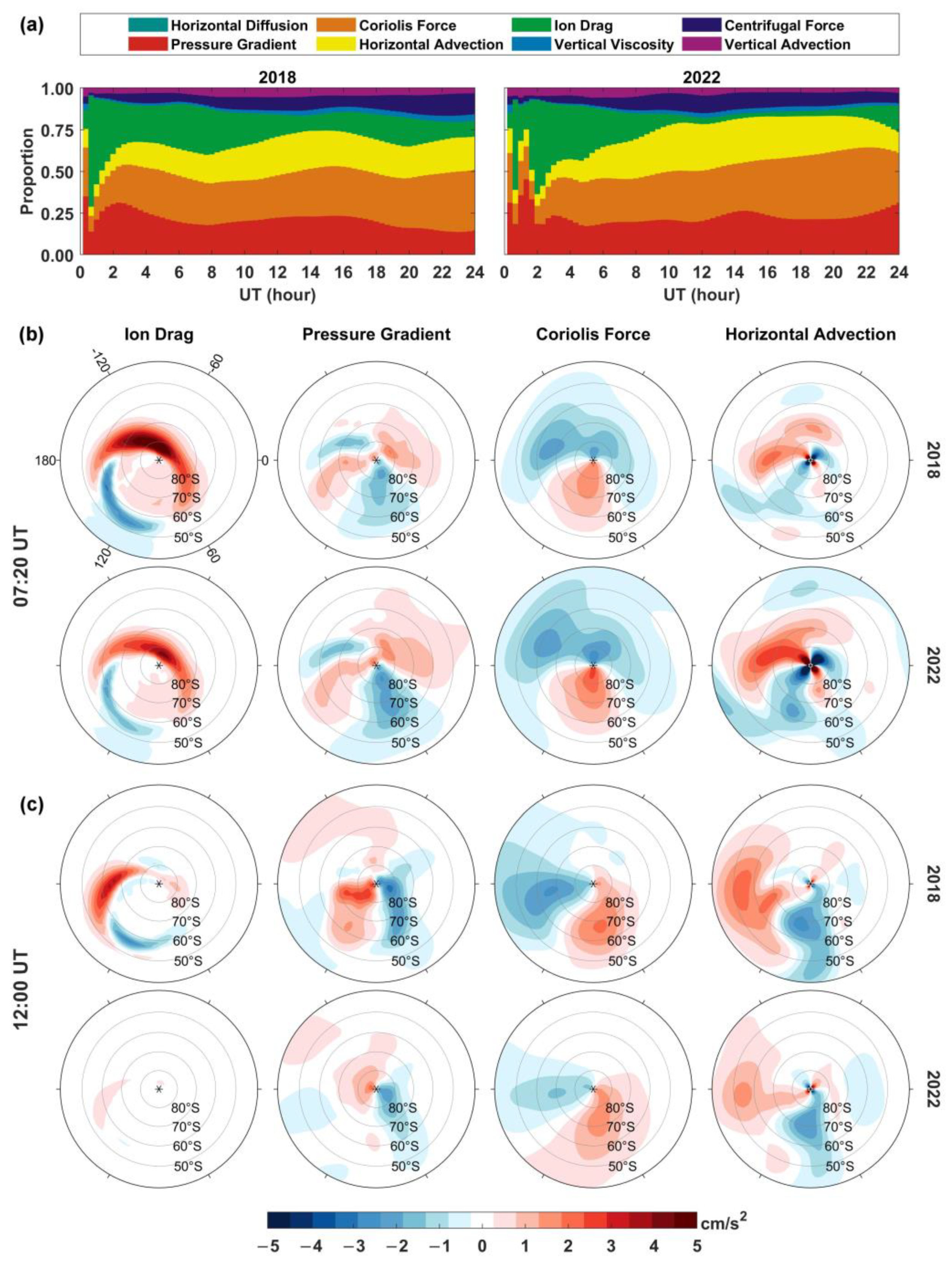
Based on the horizontal wind momentum equation given in Equations (4) and (5), the physical mechanisms leading to the differences in the horizontal winds in the two storms can be further explored. First, to identify the main physical processes affecting the horizontal wind around 130 km at high latitude in two cases, the ratios of the sum of absolute values of the eight terms in the zonal wind momentum equation to their sum were calculated separately, and their variations on the first day of the storms are given in Figure 7a. It is observed that the pressure gradient force, Coriolis force, horizontal advection, and ion drag force were the four most important physical mechanisms in both storms, where Coriolis force and horizontal advection were reaction terms. Figure 7b,c show the four acceleration terms at high latitudes in the southern hemisphere in both storms around 130 km at 07:20 and 12:00 UT. At 07:20 UT, ion drag, Coriolis force, and horizontal advection in the 2018 event already exceeded those in 2022, while the pressure gradient was still a little weaker. Thus, at the beginning of the storm, the faster high-latitude zonal wind speed at ~130 km in 2018 than in 2022 was caused by the stronger ion drag force. By 12:00 UT, shown in Figure 7c, all four terms were more powerful in 2018 than in 2022, and they all contributed to the faster zonal wind speed. The diagnostic analysis of the meridional winds shown in Figure 8 also drew the same conclusion as zonal winds. However, the Coriolis force ( f c o r U n ) and horizontal convection ( v n · V n ) are only related to the horizontal wind itself and its gradient, implying that they were not the fundamental cause of the high-latitude horizontal winds changes at ~130 km in the two storms. The stronger ion drag force first appeared. Pressure gradient force appeared later and then continued to enhance horizontal wind. In summary, the longer duration of the geomagnetic storm leads to more particle and energy input, which increases the conductivity and ion drift velocity in the high-latitude thermosphere, resulting in stronger ion drag forces. On the other hand, the longer duration induces a longer effect of Joule heating, which causes more temperature increases. The significant temperature increases are associated with the stronger pressure gradient force. Combining with a stronger pressure gradient and ion drag force resulted in faster horizontal wind speed after 08:30 UT on the first day of the storm in the 2018 event compared to those in the 2022 event. Then, the faster horizontal winds coupled with a similar wind structure resulted in greater horizontal divergence at ~130 km in the 2018 event, which pulled the faster downward vertical winds. The adiabatic heating and vertical advection processes near 110 km in the 2018 event were stronger due to the faster downward vertical winds, leading to more pronounced temperature variations. The entire process is shown in Figure 9. Therefore, for two medium storms, the effects of a storm’s duration of large Kp values is extremely important on high-latitude MLT temperature. Even if the Kp maximum of a geomagnetic storm is weak, the long duration for large Kp values can still induce a prominent MLT temperature response. It is worth noting that the Northern hemisphere also showed similar results as that in the Southern hemisphere for simulated temperature increase and physical mechanisms.

5. Summary

By comparing the temperature changes of SABER observations and TIMEGCM simulations in the MLT region around 80° S during the April 2018 geomagnetic storm and the April 2022 geomagnetic storm, the conclusion is drawn as follows: (1) The high-latitude temperature increase in the Southern hemisphere can reach 40 K in the MLT region (80 km–110 km) during the weaker and longer duration of large Kp values in the April 2018 geomagnetic storm; whereas, in the stronger and shorter-duration April 2022 event, temperature variations are relatively smaller, just less than 10 K. (2) The adiabatic heating/cooling and vertical convection that caused the temperature increases of both events are due to the downward vertical wind, which is stronger at ~−15 cm/s in the 2018 event and weaker at ~−5 cm/s in the 2022 event. (3) The larger (smaller) horizontal divergence associated with the gradient of horizontal winds around ~130 km in the 2018 (2022) storm with longer (shorter) duration produces faster (slower) downward vertical winds at the same pressure level, which can pull the vertical winds at lower altitudes and eventually lead to stronger (weaker) vertical wind disturbances below 110 km. (4) The high-latitude horizontal wind speed at ~130 km in the 2018 storm begins to exceed that in the 2022 storm at 08:50 UT (recovery phase) on the first day of the storm. (5) The more particles and energy input in the 2018 storm with a longer duration of large Kp values causes stronger ion drag force and pressure gradient force. This fundamentally results in horizontal wind speed in 2018 being roughly 1.5 times faster than that in 2022, which causes the differences in the horizontal divergence.

Author Contributions

Conceptualization, G.W. and J.L. (Jianyong Lu); methodology, G.W. and J.L. (Jianyong Lu); software, Z.L.; formal analysis, W.W., Y.T., J.L. (Jingyuan Li), S.J., Z.Z. and J.W.; resources, C.Y., F.S. and H.Z.; data curation, G.W.; writing—original draft, G.W.; writing—review and editing, J.L. (Jianyong Lu) and J.L. (Jingyuan Li); visualization, G.W., S.X., M.S., J.C. and J.Y.; supervision, J.L. (Jianyong Lu); funding acquisition, J.L. (Jianyong Lu), Y.T., J.L. (Jingyuan Li) and Z.L. All authors have read and agreed to the published version of the manuscript.

Funding

The work was supported by the National Natural Science Foundation of China (NSFC) under Grants 42004132, 42030203, and 42074183, the Startup Foundation for Introducing Talent of NUIST under Grant 2020r052, the China Geological Survey under Grants ZD20220145 and ZD20220135, the open funding of MNR Key Laboratory for Polar Science under Grant KP202104.

Data Availability Statement

The SABER-measured temperature data are available online at the SABER website (http://saber.gats-inc.com/data_services.php, accessed on 5 December 2022). The Kp index can be obtained from the CelesTrak website (http://www.celestrak.com/SpaceData/SW-All.txt, accessed on 5 December 2022). Simulation data are saved on the National Space Science Data Center (DOI: 10.57760/sciencedb.o00009.00301).

Conflicts of Interest

The authors declare no competing interest.

References

  1. Wand, R.H. Lower Thermospheric Structure from Millstone Hill Incoherent Scatter Radar Measurements 2. Semidiurnal Temperature Component. J. Geophys. Res. 1983, 88, 7211–7224. [Google Scholar] [CrossRef]
  2. Lei, J.; Burns, A.G.; Thayer, J.P.; Wang, W.; Mlynczak, M.G.; Hunt, L.A.; Dou, X.; Sutton, E. Overcooling in the upper thermosphere during the recovery phase of the 2003 October storms. J. Geophys. Res. 2012, 117, A03314. [Google Scholar] [CrossRef]
  3. Wang, N.; Yue, J.; Wang, W.; Qian, L.; Jian, L.; Zhang, J. A comparison of the CIR- and CME-induced geomagnetic activity effects on mesosphere and lower thermospheric temperature. J. Geophys. Res. Space Phys. 2021, 126, e2020JA02902. [Google Scholar] [CrossRef]
  4. Von Savigny, C.; Sinnhuber, M.; Bovensmann, H.; Burrows, J.P.; Kallenrode, M.-B.; Schwartz, M. On the disappearance of noctilucent clouds during the January 2005 solar proton events. Geophys. Res. Lett. 2007, 34, L02805. [Google Scholar] [CrossRef]
  5. Pancheva, D.; Singer, W.; Mukhtarov, P. Regional response of the mesosphere-lower thermosphere dynamics over Scandinavia to solar proton events and geomagnetic storms in late October 2003. J. Atmos. Terr. Phys. 2007, 69, 1075–1094. [Google Scholar] [CrossRef]
  6. Nesse Tyssøy, H.; Heinrich, D.; Stadsnes, J.; Sørbø, M.; Hoppe, U.-P.; Evans, D.S.; Williams, B.P.; Honary, F. Upper-mesospheric temperatures measured during intense substorms in the declining phase of the January 2005 solar proton events. Ann. Geophys. 2008, 26, 2515–2529. [Google Scholar] [CrossRef]
  7. Fang, X.; Randall, C.E.; Lummerzheim, D.; Solomon, S.C.; Mills, M.J.; Marsh, D.R.; Jackman, C.H.; Wang, W.; Lu, G. Electron impact ionization: A new parameterization for 100 eV to 1 MeV electrons. J. Geophys. Res. 2008, 113, A09311. [Google Scholar] [CrossRef]
  8. Xu, J.; Smith, A.K.; Wang, W. An observational and theoretical study of the longitudinal variation in neutral temperature induced by aurora heating in the lower thermosphere. J. Geophys. Res. Space Phys. 2013, 118, 7410–7425. [Google Scholar] [CrossRef]
  9. Yuan, T.; Zhang, Y.; Cai, X.; She, S.-Y.; Paxton, L.J. Impacts of CME-induced geomagnetic storms on the midlatitude mesosphere and lower thermosphere observed by a sodium lidar and TIMED/GUVI. Geophys. Res. Let. 2015, 42, 7295–7302. [Google Scholar] [CrossRef]
  10. Zhang, K.; Wang, W.; Wang, H.; Dang, T.; Liu, J.; Wu, Q. The Longitudinal Variations of Upper Thermospheric Zonal Winds Observed by the CHAMP Satellite at Low and Midlatitudes. J. Geophys. Res. Space Phys. 2018, 123, 9652–9668. [Google Scholar] [CrossRef] [Green Version]
  11. Zhang, K.; Liu, J.; Wang, W.; Wang, H. The Effects of IMF Bz Periodic Oscillations on Thermospheric Meridional Winds. J. Geophys. Res. Space Phys. 2019, 124, 5800–5815. [Google Scholar] [CrossRef]
  12. Liu, X.; Yue, J.; Wang, W.; Xu, J.; Zhang, Y.; Li, J.; Russell, J.M., III; Hervig, M.E.; Bailey, S.; Nakamura, T. Responses of lower thermospheric temperature to the 2013 St. Patrick’s Day geomagnetic storm. Geophys. Res. Lett. 2018, 45, 4656–4663. [Google Scholar] [CrossRef]
  13. Li, J.; Wang, W.; Lu, J.; Yuan, T.; Yue, J.; Liu, X.; Zhang, K.D.; Burns, A.G.; Zhang, Y.; Li, Z. On the responses of mesosphere and lower thermosphere temperatures to geomagnetic storms at low and middle latitudes. Geophys. Res. Lett. 2018, 45, 10–128. [Google Scholar] [CrossRef]
  14. Li, J.; Wang, W.; Lu, J.; Yue, J.; Burns, A.G.; Yuan, T.; Chen, X.; Dong, W. A modeling study of the responses of mesosphere and lower thermosphere winds to geomagnetic storms at middle latitudes. J. Geophys. Res. 2019, 124, 3666–3680. [Google Scholar] [CrossRef]
  15. Zou, Z.; Xue, X.; Yi, W.; Shen, C.; Yang, C.; Tang, Y.; Chen, T.; Dou, X. Response of the high-latitude upper mesosphere to energetic electron precipitation. Astrophys. J. 2020, 893, 55. [Google Scholar] [CrossRef]
  16. Sun, M.; Li, Z.; Li, J.; Lu, J.; Gu, C.; Zhu, M.; Tian, Y. Responses of Mesosphere and Lower Thermosphere Temperature to the Geomagnetic Storm on 7–8 September 2017. Universe 2022, 8, 96. [Google Scholar] [CrossRef]
  17. Mlynczak, M.G. Energetics of the mesosphere and lower thermosphere and the SABER experiment. Adv. Space Res. 1997, 20, 1177. [Google Scholar] [CrossRef]
  18. Russell, J.M., III; Mlynczak, M.G.; Gordley, L.L.; Tansock, J.; Esplin, R. An overview of the SABER experiment and preliminary calibration results. Proc. SPIE-Int. Soc. Opt. Eng. 1999, 3756, 277–288. [Google Scholar]
  19. Remsberg, E.E.; Marshall, B.T.; Garcia-Comas, M.; Krueger, D.; Lingenfelser, G.S.; Martin-Torres, J.; Mlynczak, M.G.; Russell III, J.M.; Smith, A.K.; Zhao, Y.; et al. Assessment of the quality of the Version 1.07 temperature-versus-pressure profiles of the middle atmosphere from TIMED/SABER. J. Geophys. Res. 2008, 113, D17101. [Google Scholar] [CrossRef]
  20. Roble, R.G.; Ridley, E.C.; Richmond, A.D.; Dickinson, R.E. A coupled thermosphere/ionosphere general circulation model. Geophys. Res. Lett. 1988, 15, 1325–1328. [Google Scholar] [CrossRef]
  21. Roble, R.G.; Ridley, E.C. A thermosphere-ionosphere-mesosphere-electrodynamics general circulation model (time-GCM): Equinox solar cycle minimum simulations (30–500 km). Geophys. Res. Let. 1994, 21, 417–420. [Google Scholar] [CrossRef]
  22. Heelis, R.A.; Lowell, J.K.; Spiro, R.W. A model of the high-latitude ionospheric convection pattern. J. Geophys. Res. 1982, 87, 6339–6345. [Google Scholar] [CrossRef]
  23. Li, G.; Ning, B.; Zhao, X.; Sun, W.; Hu, L.; Xie, H.; Liu, K.; Ajith, K.K. Low latitude ionospheric TEC oscillations associated with periodic changes in IMF Bz polarity. Geophys. Res. Lett. 2019, 46, 9379–9387. [Google Scholar] [CrossRef]
  24. Liu, J.; Wang, W.; Burns, A.; Yue, X.; Zhang, S.; Huang, C. Profiles of ionospheric storm-enhanced density during the 17 March great storm. J. Geophys. Res. Space Phys. 2016, 121, 727–744. [Google Scholar] [CrossRef]
  25. Liu, X.; Yue, J.; Xu, J.; Garcia, R.R.; Russell, J.M., III; Mlynczak, M.; Wu, D.; Nakamura, T. Variations of global gravity waves derived from 14 years of SABER temperature observations. J. Geophys. Res. Atmos. 2017, 122, 6231–6249. [Google Scholar] [CrossRef]
  26. Xu, J.; Smith, A.K.; Liu, M.; Liu, X.; Gao, H.; Jiang, G.; Yuan, W. Evidence for nonmigrating tides produced by the interaction between tides and stationary planetary waves in the stratosphere and lower mesosphere. J. Geophys. Res. Atmos. 2014, 119, 471–489. [Google Scholar] [CrossRef]
Figure 1. The difference between the zonal running SABER temperature (first row) during two geomagnetic storms in April 2018 (the left column) and April 2022 (the right column) and the average temperature of the two days before the storms (18–19 April 2018 and 8–9 April 2022, respectively) in the altitude ranges of 80–110 km from 77.5° S to 82.5° S. The second row is similar to the first row, but the data are simulated by TIMEGCM driven by real geomagnetic conditions (rkp). The third row shows the variations in temperature obtained by subtracting the simulation driven by constant geomagnetic conditions (ckp) from the simulation driven by real geomagnetic conditions (rkp). The blue lines are the real Kp values. The red lines are the quiet time Kp values as the driving condition of the ckp simulation. The two ckp are 1+ for 20 April 2018, and 2 for 10 April 2022, respectively. Then the constant Kp values are set the same as the real ones.
Universe 09 00086 g001
Figure 2. The first three rows correspond to the temperature difference (rkp−ckp) for TIMEGCM simulations at 01:00 UT (first row), 12:00 UT (second row), and 18:00 UT (third row) on the first day of the storm (20 April 2018 on the left column and 10 April 2022 on the right column) at 110 km in the southern hemisphere. The fourth row is the same as the first three rows but at 12:00 UT on the second day of the storm (21 April 2018 on the left column and 11 April 2022 on the right column). The black asterisks mark the locations of the satellite observation points at the corresponding time. The green dots mark the position of (78.75° S, 60° E), which is used for the subsequent thermodynamic diagnostic analysis.
Universe 09 00086 g002
Figure 3. Storm-time differences (rkp−ckp) in total heating terms and major heating terms at the location of (78.75° S, 60° E) in the altitude ranges of 80 km to 110 km in the two storms: total heating, adiabatic heating/cooling, vertical heat advection, horizontal heat advection, and Joule heating.
Universe 09 00086 g003
Figure 4. Storm-time differences (rkp−ckp) in vertical velocity, vertical term, and horizontal term at the location of (78.75° S, 60° E) in the altitude ranges of 90 km to 150 km in the two storms. The vertical velocity was the sum of the vertical term and horizontal term. The red dashed lines represent 110 km. The black lines represent the zero value. The green asterisks corresponded to the time and altitude of 14:20 UT and ~130 km, respectively.
Universe 09 00086 g004
Figure 5. The left column corresponds to the 2018 storm event and the right column represents the 2022 storm event. The different rows show the effects of magnetic storms on the total horizontal divergence term (first row, same as the third row in Figure 4), the zonal component of the horizontal divergence term (second row), the meridional component of the horizontal divergence term (third row), the zonal wind (fourth row), and the meridional wind at 14:20 UT around 130 km. The green dot is located at (78.75° S, 60° E), which is the location where the kinetic diagnostic analysis is performed. The arrows show the magnitude and direction of the horizontal wind. The black asterisks mark the locations of the South Pole.
Universe 09 00086 g005
Figure 6. (a) The red line represents the Kp values on 20 April 2018 and the green line stands for the Kp values on 10 April 2022. (b) Each grid zonal wind velocity during the 2018 storm is divided by the 2022 zonal wind velocity on the same grid to obtain the ratio of the zonal wind speed for two events in each grid. Then, the number of grids are counted in each ratio and its proportion to the total number of grids is calculated. The figure shows the statistical distribution of zonal wind ratios (2018/2022) of grids from 50° S to 90° S in the two events over time, where >1 (<1) represents a larger zonal wind velocity in the 2018 (2022) storm. (c) Same as (b), but corresponding to the meridional wind.
Universe 09 00086 g006
Figure 7. (a) The ratios of eight acceleration terms in the zonal wind as shown in Equation (4). (b) Mainly zonal acceleration terms: ion drag force (first column), pressure gradient force (second row), Coriolis force (third row), and horizontal advection (fourth row) for the 2018 event (first row) and 2022 event (second row) around 130 km on the first day of the storm (April 20 for the 2018 event and April 10 for the 2022 event) at 07:20 UT. (c) Same as (b), but corresponding to 12:00 UT. The black asterisks mark the locations of the South Pole.
Universe 09 00086 g007
Figure 8. (a) The ratios of eight acceleration terms in the meridional wind as shown in Equation (4). (b) Mainly meridional acceleration terms: ion drag force (first column), pressure gradient force (second row), Coriolis force (third row), and horizontal advection (fourth row) for the 2018 event (first row) and 2022 event (second row) around 130 km on the first day of the storm (April 20 for the 2018 event and April 10 for the 2022 event) at 07:20 UT. (c) Same as (b), but corresponding to 12:00 UT. The black asterisks mark the locations of the South Pole.
Universe 09 00086 g008
Figure 9. Schematic figure of the physical process of temperature increases due to geomagnetic storms with longer duration.
Universe 09 00086 g009
Disclaimer/Publisher’s Note: The statements, opinions and data contained in all publications are solely those of the individual author(s) and contributor(s) and not of MDPI and/or the editor(s). MDPI and/or the editor(s) disclaim responsibility for any injury to people or property resulting from any ideas, methods, instructions or products referred to in the content.

