Abstract
In this paper, we construct a solvable toy model of the quantum dynamics of the interior of a spherical black hole with falling spherical scalar field excitations. We first argue about how some aspects of the quantum gravity dynamics of realistic black holes emitting Hawking radiation can be modeled using Kantowski–Sachs solutions with a massless scalar field when one focuses on the deep interior region (including the singularity). Further, we show that in the regime, and in suitable variables, the KS model becomes exactly solvable at both the classical and quantum levels. The quantum dynamics inspired by loop quantum gravity is revisited. We propose a natural polymer quantization where the area a of the orbits of the rotation group is quantized. The polymer (or loop) dynamics is closely related to the Schroedinger dynamics away from the singularity with a form of continuum limit naturally emerging from the polymer treatment. The Dirac observable associated with the mass is quantized and shown to have an infinite degeneracy associated with the so-called -sectors. Suitable continuum superpositions of these are well-defined distributions in the fundamental Hilbert space and satisfy the continuum Schroedinger dynamics.
1. Motivation
The fate of the singularities of general relativity is a central question for quantum gravity that concerns important physical situations such as those arising in (Big Bang) cosmologies and black hole formation and evaporation. One of the central features of loop quantum gravity is the inherent discreteness of quantum geometry at the Planck scale. The lack of smoothness of the geometry at the fundamental level challenges the classical view of the singularities of general relativity as a frontier of spacetime geometry, and strongly suggests the possibility of a microscopic dynamical description that could define dynamics beyond the limit where classical description fails.
The history of the approach starts with the discovery of Ashtekar’s connection variables, which first suggested that the quantum dynamical evolution equations of gravity might admit a background independent finite and nonperturbative formulation [1,2]. This initial suggestion grew into the approach of loop quantum gravity (LQG) with the contributions of many (for reviews and text books, see [3,4,5,6,7]). The LQG approach has produced insights about the possible nature of matter and geometry at the Planck scale and has led to new ideas about the origin of black hole entropy, the generation of quantum effects in early cosmology, and stimulated hopes about the possible regularizing role of Planckian granularity (for quantum field theory and gravity). However, a clear understanding of the question of the fate of singularities in realistic physical situations has remained a difficult one, as addressing it would actually require the (still lacking) complete dynamical control of LQG in situations involving matter and geometric degrees of freedom in the deep ultraviolet regime in full generality.
Nevertheless, the view that the evolution across singularities should be well behaved has become consensual in the field over time thanks to the accumulated experience in simple low-dimensional and symmetry-reduced models of black holes and cosmology. Professor Abhay Ashtekar has been one of the driving forces along this path, and the main defender of the view (to which we adhere) that dynamics across the would-be-singularity should be well-defined in quantum theory. It is a pleasure to contribute to this special issue with this work that, we believe, is representative of this standpoint.
The first examples of singularity avoiding models were found in the context of quantum cosmology by Martin Bojowald [8]. This seminal work grew later into a large number of contributions in the field now known as loop quantum cosmology [9,10,11]. Even in these simple models, the quantum dynamics can be rather involved. However, it was soon realized [12] that effective semiclassical equations could be used to describe the dynamics across the singularity and that these equations were quite easy to describe. The domain of applicability of these techniques was extended in a variety of manners to models involving black holes [13,14,15,16,17,18,19,20] (for quantum modifications inspired by other approaches, see [21,22,23]). In many of the latter cases, the natural starting point has been to consider the quantum dynamics of the interior of spherically symmetric and static spacetimes of the Kantowski–Sachs type (the Schwarzschild black hole’s interior in the vacuum case). In all these cases, the interior singularity is removed and replaced by a quantum transition across what would have been the singularity in the classical description realizing aspects of existing scenarios [24,25,26,27].
Simple models are nice, as they illustrate possibly generic features of the general situation. However, they carry the drawback of being often removed, by the very symmetry assumptions that simplify them, from the realistic physical situations about which one would like to gain non-trivial insights. Moreover, when it comes to black holes, most of the studies have focused on effective dynamical descriptions, whereas quantum dynamics has received less attention due to its often insurmountable complexity even in simple models. For instance, concerning the first drawback, we know that real black holes are not time translationally invariant due to the expected presence of Hawking evaporation (in contrast with the static nature of many of the quantum black hole models) and that all symmetry assumptions must fail near the singularity when the back-reaction of Hawking particles correlated with the outside radiation is properly taken into account (see [28] for further discussion of this issue). When it comes to the second drawback, even when effective descriptions can provide the dynamical evolution of the spacetime geometry with matter fields on it, its classical nature precludes the analysis of genuine quantum phenomena such as entanglement and other quantum information issues of the highest interest from the perspective of Hawking’s evaporation (e.g., the longstanding information puzzle or the question of the fate of unitarity in black hole evaporation). Even when our model will not resolve the first limitation, we believe that it provides a humble step in the right direction. Concerning the second, we will see that the quantum dynamics is fully accessible in our simple model, opening the road for exact calculations in the quantum realm.
The interior region of a Schwarzschild black hole of mass M can be seen as a homogeneous anisotropic cosmological model where the r=constant surfaces (in the usual Schwarzschild coordinates) are Cauchy surfaces of homogeneity, where any two arbitrary points can be connected along orbits of the isometry group that involves space-like translations along the staticity killing field and the rotations associated with spherical symmetry. Models with these isometries will be refereed to as Kantowski–Sachs (KS) models [29]. They include not only the Schwarzschild black hole’s interior geometry (vacuum case) but also the Reissner–Nordstrom black hole’s interior geometry (in the Einstein–Maxwell case), and other solutions, depending of the type of matter that one decides to couple to the system. In this paper, we would like to emphasize the fact that Kantowski–Sachs models (with a massless scalar field coupling) define a natural toy model capturing some (possibly interesting) aspects of the dynamics and back-reaction of matter near the singularity of realistic black holes that Hawking radiate and evaporate. The model can certainly not replace the full dynamical description of a generic gravitational collapse in the full theory, as it remains a toy model with finitely many degrees of freedom. However, we will argue, it can handle in a simplistic way some dynamical aspects that might be relevant when discussing questions in the context of evaporating black holes.
The physical situation where black hole formation and evaporation takes place is illustrated by the Ashtekar-Bojowald paradigm spacetime whose Penrose diagram is shown in Figure 1.
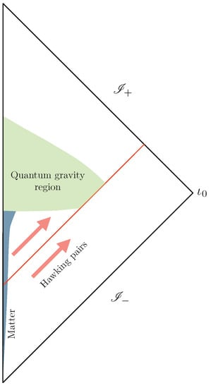
Figure 1.
The Ashtekar–Bojowald paradigm.
1.1. Scalar Excitations Falling Inside a Schwarzschild Black Hole: The Deep Interior Regime
Let us consider a free test point particle (with no angular momentum) falling into the interior of a Schwarzschild black hole. As the particle approaches the singularity—in a description on an r equal constant slicing of the interior—one expects its wave function to become better and better approximated by a translationally invariant wave function, since the expansion in the space-like killing direction diverges for . If this conclusion is correct, then it means that zero-angular-momentum test particles can be approximated by excitations of the type that can be accommodated in the dynamical framework of the KS cosmologies (at least in the sense of a near-singularity approximation). One can be quantitative about this intuition as follows: Free test particles with four wave vectors on the Schwarzschild background are associated with the conserved killing energy . We are assuming that the particle has zero angular momentum, which implies that its wave function is already translationally invariant in the directions transverse to on the r-slices. The wave function can only vary in the direction of the killing , and the component of the physical momentum in this direction is given by
which vanishes in the limit . The wavelength of such a particle diverges, and thus, particles without angular momentum are better and better represented by translationally invariant excitations as one approaches the singularity. These are precisely the kind of homogeneous configurations that can be described in the KS framework.
This simple implication deduced from the idealized notion of test particle can be made more precise by looking at the analogous features of scalar field excitations (solutions of the Klein–Gordon equation). Indeed, the simplistic argument given here can be made precise in the field theoretical context, as we will show in what follows.
Solutions of the Klein–Gordon Equation in the Deep Interior Region
Here we argue that the Kantowski–Sachs model (described in detail in Section 2) coupled to a massless scalar field faithfully captures the dynamics of a Klein–Gordon excitation falling into the deep interior region of a Schwarzschild black hole. We do this by analyzing the behavior of solutions of the Klein–Gordon equation on the Schwarzschild background in the regime. We focus on the spherically symmetric solutions and show that they become homogeneous on r=constant surfaces as and thus can be accommodated in the framework of KS configurations. This implies that the KS system can be used to model the dynamics and (most importantly) the back-reactions of such (zero angular momentum) scalar configurations falling into the deep interior region of spherically symmetric black holes.
Let us first start by approximating the Schwarzschild metric in the deep interior region as
We chose coordinates such that the time-radial part of the metric is conformally flat. Remarkably, in the deep interior region, this is achieved by switching to area variables (the well-known tortoise coordinate is actually proportional to near the singularity). With these variables, the metric becomes
with , , and . The Klein–Gordon equation for a massless scalar field then reads
To solve it, we make the usual ansatz
which reduces the Klein–Gordon equation to
For the spherical modes , one obtains
with and Bessel functions and and constants. As we will prove in Section 2, these solutions match nicely with solutions of the KS model (mentioned at the end of the introduction). This follows from two complementary properties of the solutions of the Klein–Gordon equation. On the one hand, the near singularity limit of the quantity (simply related to the KS momentum variable, as we will see in Section 2),
is finite and independent of . On the other hand, the t dependence of the Klein–Gordon solutions is ’ironed’ by the infinite expansion of the geometry in the direction: the region where the solution has a significant (order-one) change corresponds to a length scale (in agreement with the infinite redshift effect captured in Equation (1)). Therefore, in a length scale along the background killing field direction , and in the deep interior region , the solutions of the Klein–Gordon equations can be considered as homogeneous, and therefore compatible with initial data that would be admissible in the KS model.
We will see in Section 2 that the momentum variable in the KS model is simply related to the quantity whose limit was considered in the previous paragraph, as it is defined as
where the pre-factors arise form the Hamiltonian analysis of Section 2 and is an IR cut-off scale naturally associated in the previous discussion to the scale . It follows from the previous considerations that
in the region of interest. One can relate the previous quantity to the average ’energy density’ on the r=constant hyper-surfaces as one approaches the singularity (this will be simply related to the KS Hamiltonian that will be defined in the following section). Namely,
where the scale enters the definition of the average in the time direction. For concreteness, one can match to the wavelength of the excitation, and the previous result will already hold (of course it holds for ).
For completeness, we give the limiting behavior of solutions in the non-spherical case. For the non-spherical modes, one can neglect the term containing the frequency in Equation (7) in analyzing the small a behavior of solutions. If we do so, we obtain for
Solutions diverge logarithmically (as ) for . This holds both for spherically symmetric and for nonspherically symmetric solutions, as it follows from the asymptotic behavior of the Bessel functions or from the finiteness of in the spherical case. The mild character of the divergence was emphasized in [30,31] as an attractive, possibly interesting property when one considers the definition of the associated quantum operators in quantum field theory (in view of a possible definition of semiclassical gravity). Here, we simply point out that such simple behavior allows for bridging to a solvable KS model to understand aspects of the back-reaction of classical (and quantum) excitations falling into a spherically symmetric black hole.
2. The Kantowski–Sachs Spacetime Coupled with a Massless Scalar Field
In this section, we revisit the construction of the phase space of the KS model by performing the canonical analysis of the associated symmetry-reduced model where staticity and spherical symmetry are imposed from the onset (in Section 2.1). To improve the clarity of the presentation, we simply start from the vacuum case—whose solutions are isomorphic to the interior Schwarzschild solutions—and later couple the system to a scalar field without mass. We express variables in terms of the usual Schwarzschild-like coordinates. In Section 2.2, we present a truncation of the Hamiltonian, and we show in Section 2.3 that it defines a tractable approximation of the dynamics in the region of the interior of physically realistic black holes. We call this regime the deep interior dynamics. In Section 2.4, we show that the regime of applicability of the model includes the physically interesting situation of Hawking scalar excitations with zero angular momentum falling inside of the black hole.
2.1. Symmetry-Reduced Covariant Phase Space
It is well-known that for a spherically symmetric and static spacetime, the line element can be written without any loss of generality as
It follows that the Eintein–Hilbert action (with the appropriate boundary term that renders it differentiable) becomes
where the dot denotes the derivative with respect to r and is a cut-off in the noncompact space-like direction that regularizes the dynamical system. The cut-off will be associated a natural meaning in modeling the fate of zero angular momentum excitations falling inside the black hole. In the deep interior region , we will take for (the typical frequency in the Hawking spectrum of a macroscopic black hole of mass M). One can easily verify that the variations of the action lead to the Schwarzschild solutions
and the symplectic potential (stemming from the on-shell evaluation of the action variation)
and symplectic structure
Instead of working directly with the physical phase space parametrized by the Dirac observables and M, it will be convenient for us to work with kinematical variables and constraints for the moment. This is because of the usual difficulty in linking the timeless physical phase space with a classical intuition based on spacetime geometry. To avoid such difficulties, we would like to have a notion of parametrized ’time evolution’, which in our context will take the form of an area radius evolution. Thus, we take the integrand of (15) as the Lagrangian of the spacetime subsystem
Alternatively, we couple the system to a massless scalar field by adding the matter action
The conjugate momenta to and are given by
and the primary Hamiltonian, defined by , becomes
From the expression of the conjugate momenta (21), we identify the constraints
and the secondary Hamiltonian
where and are Lagrange multipliers. One can show that the stability of the two constraints (23) can be ensured by fixing the associated Lagrange multipliers; i.e., the constraints (23) are second class and can be explicitly solved, leading to
Thus, the secondary Hamiltonian (24) reduces to
The previous equation encodes the KS dynamics of geometry coupled to a massless scalar field. The relevant solutions for physical applications correspond to small departures from the vacuum Schwarzschild solutions representing macroscopic black holes with scalar field perturbation falling inside. We will further simplify the system by focusing on what we call the deep interior region, , where M is the mass scale defined by the corresponding black hole solution perturbed (in the sense of Section 2.3 and Section 2.4) by the presence of matter. It is in this regime where the solutions of the KS system faithfully describe the dynamics of a spherically symmetric scalar perturbation (representing, for instance, a Hawking particle) as it falls towards the interior singularity. The KS Hamiltonian evolution matches, in this sense, the test-field evolution (the Klein–Gordon solutions on the Schwarzschild background fixed nondynamical background) and incorporates, as a simplified model, aspects of the back-reaction that are expected to become more important as one approaches the singularity.
2.2. The Deep Interior Dynamics
We are interested in the dynamical evolution in the regime. In addition, we will use the present dynamical system to model (in a suitable approximation) the back-reaction of a Hawking quantum falling into a black hole singularity. Hawking particles do not correspond to static excitations as the one we can model with the symmetry assumptions of the present section. However, as argued in Section 1.1, when spherically symmetric, these particles look more and more static, as seen by a radially freely falling observer in the limit . This is the reason why we are interested in such a regime of the present dynamical system. In the next, section we will study the classical solution of the model using perturbation theory in the parameter —as will be assumed to be much smaller to in applications—and show that the dynamics simplifies in the deep interior region. The simplification occurs due to the negligible effect of the last term in the expression of the Hamiltonian (26): more precisely, in the deep interior region, the Hamiltonian is well approximated by
This toy theory reflects the dynamics of the leading order in an expansion near . Order effects could be included in perturbation theory near , in which case the term we dropped would correspond to the perturbation Hamiltonian. The consistency of this truncation will be shown in Section 2.3.
The system we are dealing with has no gauge symmetries, as the radial reparametrization symmetry has been gauged fixed with the metric ansatz (14) by choosing the area radius as time. In order to recover the structure of a gauge theory, with clear analogy to the full theory of LQG, it will be convenient ’reparametrize’ the system by promoting the area radius r to a degree of freedom with conjugate momentum and adding a scalar constraint . The phase space is therefore extended to , and the number of degrees of freedom is preserved by the inclusion of the Hamiltonian constraint:
In this approximation, one can show that we have the following Dirac observables:
It will be convenient to make the following canonical transformation and thereby introduce what we call the deep interior variables:
and—in trying to introduce the kinematical structure proper to loop quantum gravity—to adopt the area a of the surfaces of constant r, namely,
as new dynamical variables. With this choice, the phase space is described by the geometric variables and with Poisson brackets
and by the matter variables and for which
with all the other Poisson brackets equal to zero. In the new variables, the deep interior dynamics Hamiltonian constraint (28) becomes
The previous constraint is central in the rest of the paper. We will see that it leads to a fully controllable dynamics both at the classical level and the quantum level. Indeed, the dynamics is exactly solvable in the vacuum case, and it can be dealt with in perturbation theory for the case where the scalar field is excited. In the next section, we will justify the truncation that took us from (26) to (27) (and finally, to the constraint (33)) using perturbation theory. In Section 2.4, we will show that the perturbative regime is consistent with the conditions that make our model applicable to the description of a spherically symmetry Hawking particle falling into a Schwarzschild black hole during evaporation.
2.3. Perturbative Solutions in and the Dynamics in the Deep Interior Region
Exact KS solutions with scalar fields have been studied in the past (see for instance [32]). KS coupled to scalar fields does not lead necessarily to (asymptotically flat) back hole spacetimes globally speaking. However, we will show here that solutions can be interpreted in terms of perturbations of a vacuum Schwarzschild solution in the deep interior region in the regime where . We will also show that in that regime the Hamiltonian (26), and the equations it generates, can be well approximated by (27). This will lead to a simple solvable system, both at the classical and quantum levels, which can be used to model aspects of the physics of (zero angular momentum) scalar particles falling into a spherically symmetric black hole (possibly useful in view of describing aspects of Hawking radiation). We analyze the system in first-order perturbation theory in .
In order to best organize the perturbative equations, we replace by , where is a smallness parameter. We introduce the following expansion of the relevant dynamical quantities:
and write the equations of motion for them by keeping terms up to order . Starting from
with given in Equation (26), one can solve the equations order by order with solutions
The function is recovered from the constraint (23) and gives
Note that the Schwarzschild solution with mass M and conjugate momentum —as in (16)—is recovered in the leading order. Consistency of the perturbative treatment requires the ratio of first-to-leading order contributions to remain small, namely,
in the regime . The logarithmic behavior of the right-hand side of the previous equations is not a threat, as the classical solutions are not to be trusted for r near the Planck scale. Therefore, assuming , we conclude that our analysis is consistent as long as
which is always valid in the usual macroscopic black hole regime . Similarly, note that the ratio of the last term in the Hamiltonian (26) to the leading first term is exactly , which in the same regime is , as seen from (39). This suggests that one can simplify the dynamics (if interested in the deep interior region ) and use the Hamiltonian
This expectation is confirmed by the analysis of the Hamiltonian flow generated by in the relevant regime. One might be slightly uncomfortable with the UV cut-off used in devising conditions such as (41), after all the classical equations predict a singular evolution when , and in this limit, the right-hand side of the Equation (40) actually blows up, invalidating in appearance the perturbative analysis. We will see that the quantum dynamics across the classical singularity is actually well-defined. Moreover, we will also see that there are exact effective equations describing the evolution of the expectation value of semiclassical states across as well. These equations imply that the counterpart of the right-hand side of (40) not only does not diverge but rather tends to zero when quantum effects are included.
2.4. Validity of Perturbation Theory in View of Applying the Model to Hawking Pairs Produced by a Macroscopic Black Hole
Here, we argue for the validity of the perturbation theory analysis of the previous section in the context of applications of the KS model to the quantum dynamical description of scalar field excitations falling inside a Schwarzschild black hole during Hawking evaporation. The assumptions here are: First is the usual assumption that the gravitational collapse has formed a spherical black hole with mass . Second, the Hawking pairs produced by such a macroscopic black hole can be described as test field excitations on a stationary Schwarzschild geometry far away from the singularity. Finally, we restrict our attention to spherically symmetric Hawking pairs which are the only ones that can be mapped to the spherically symmetric KS configurations. This is not a serious restriction, given that most of the Hawking radiation is emitted in such modes [33].
The following discussion can be framed in the context of Figure 2 where Hawking pairs are represented by the red arrows. The stationarity of the background implies that the (test field) current is conserved, where is the stationarity killing field that in the adapted coordinates that we use here is simply given by , and is the energy momentum tensor of the scalar field1. Conservation of energy leads to the expectation that when a Hawking particle is detected at with a given energy = (which coincides with the associated killing conserved quantity), a Hawking partner with (killing), energy falls into the black hole singularity, reducing the mass of the black hole by . A more precise field theoretical expression of this is that the flux of the (expectation value of) energy-momentum current at infinity, in the state of the field after the detection of the particle at , equals the negative of the flux of the same current on (for instance) a constant hyper-surface . Namely,
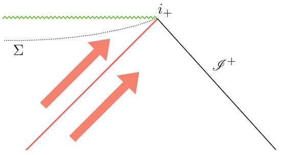
Figure 2.
Hawking pairs (red arrows) produced in a black hole spacetime with are described as test field excitations on a background spacetime that is idealized by a stationary black hole solution in the region of the Penrose diagram away from the collapsing matter and containing . Stationarity implies the existence of a conserved energy-momentum current used, in this paper, to relate the value of in the KS model to the frequency of the emitted particle at and (via Hawking temperature) to the black hole mass M. The surface represents an r=constant surface in the interior (denoted in the main text).
Using our coordinates to write explicitly the integrand on the left-hand side while pushing to the region where comparison with the KS regime is possible (a constant r such that ), we get
where the right-hand side of the last equality comes from the evaluation of the energy flux of a Hawking particle, and in the evaluation of the left-hand side, we used that for (see for instance (11)). The scalar field behaves like
The result in (44) follows also from the assumption that . By pushing the integral to its largest possible value when , we conclude that energy conservation (encoded in (44)) implies the bound
which is consistent with the condition for the validity of perturbation theory (40). We see that the physical context provided by the problem of Hawking evaporation precisely justifies the simplifying assumptions that led to (33). Notice also that the fiducial length scale acquires in such a physical situation an operational meaning as well.
A generalization of the analysis of the present Section 2 to a wider class of close to stationary black holes is certainly very appealing. Even though it is clear that the tools employed here would not apply to black hole spacetimes with angular momentum (due to the breaking of spherical symmetry), one could entertain the possibility of including an electric charge without leaving the general framework of this work. However, such an apparently simple extension will reserve challenging new aspects. The first qualitative new feature is that the singularity becomes timelike in the unperturbed black hole. However, when a scalar field perturbation is added its back reaction is expected to produce the phenomenon of mass inflation [34] near the Cauchy horizon of the unperturbed background. This completely changes the global features of a realistic charged black hole interior in a way that would seem to preclude the applicability of the present methods. More precisely, if we use the Reissner–Nordstrom background black hole geometry as a basis for the present discussion—noting that the presence of mass inflation already implies that strong deviations from the Reissner–Nordstrom interior solution are to be expected—the true would-be singularity should materialize near the location of the Cauchy horizon. However, close to the Cauchy horizon scalar field, modes with frequency are expected to be infinitely blue-shifted, precluding the type of approximation available in the present case. This makes such exploration highly non-trivial, even when certainly interesting.
3. A Natural Polymer Quantization of the Deep Interior Dynamics
In previous sections, we have shown that the Hamiltonian constraint (33) describes the deep interior dynamics of scalar excitations without angular momentum falling into a macroscopic Schwarzschild black hole. The approximations used are based on assumptions that are satisfied by the (spherically symmetric) Hawking excitations produced during black hole evaporation. Thus, the simplified dynamics in the deep interior region, which will turn out to be analytically solvable (both at the quantum and classical level), offers a toy scenario to analyze key questions of black hole evaporation in a controlled scenario. We will show in this section that there is natural polymer quantization of the deep interior dynamics with remarkable simple properties such as: (like in the full theory of LQG) the discreteness of the area of constant area surfaces, a well-defined quantum dynamics across the singularity, an effective classical description, and a direct (to our knowledge novel) link with the continuum representation. The polymer quantization we propose does not suffer from the usual ambiguities associated with the so-called holonomy corrections [35], as the Hamiltonian constraint evolution has (in our simple model) a clear-cut geometric interpretation that allows for a unique polymerization that is compatible with the continuum limit (defined by the Schroedinger representation). This special geometric property arises from the fact that the Hamiltonian constraint is linear in the momentum conjugate to the area of the spheres whose spectrum is discrete in our polymer representation. Ambiguities remain in the form of the so-called inverse volume corrections, which are necessary if one defines the quantum dynamics across the singularity.
3.1. Sketch of the Schrodinger quantization
In the standard Schrodinger representation, one would quantize the phase space of Section 2.1 by promoting the variables to self adjoint operators:
in the kinematical Hilbert space is , equipped with the usual inner product
where we have chosen the momentum representation for the scalar field for convenience (as is one of the constants of motion of the system). Eigenstates of the operator are interpreted as distributions (they are not in the Hilbert space), and one usually writes
with and form an orthonormal basis
The dynamics is imposed by solving the Hamiltonian constraint (33), which, in the present representation, takes the precise form of a Schrodinger equation in the area variable a, namely,
As usual, solutions of the constraint are certainly not square-integrable in the a-direction; thus, physical states are outside of the kinematical Hilbert. The physical Hilbert space is defined as the space of square integrable functions of m and at fixed time a——with inner product
which is preserved; i.e., it is independent of a, by the Schrodinger Equation (evolution is unitary in a).
Two important remarks are in order: First, note that we are formulating in detail the dynamics of the system in the near singularity approximation. The physical reason for this is that (as argued previously) it is only in this approximation that the system can be compared with a (spherically symmetric) black hole with spherically symmetric excitations falling inside. A side gain is also the simplification of the dynamics which will allow us a simpler quantization and the analysis of the possibility of a well-defined dynamics across the singularity when we undergo the LQG inspired quantization. One could, however, consider the quantization of the minisuperspace system without the near-singularity approximation. In that case, one would need to write a Schroedinger equation using the Hamiltonian (26), now genuinely time-dependent (r-dependent), for which unitary evolution would involve path ordered exponentials (as the Hamiltonian does not commute with itself at different r values). In addition, one would need to work with either variables or variables without the luxury of the simplifications introduced by the use of the near singularity variables (30).
3.2. The Polymer Quantization
We define now a representation of the phase-space variables that incorporates a key feature of the full theory of LQG: the area quantization. Such representation closely mimics the structure of the quantum theory in the fundamental theory in such a way that the area variable a acquires a discrete spectrum. Mathematically, this is achieved by replacing the structure of the inner product in the variable by the inner product of the Bohr compactification of the phase-space dimension. More precisely, one substitutes the kinematical inner product in the Schroedinger representation (47) by
With this inner product, periodic functions of with an arbitrary period are normalizable, and the conjugate a-representation acquires the property of discreteness in a way that closely mimics the structure of the fundamental theory of loop quantum gravity [11]. In particular, eigenstates of exist
with . These states form an orthonormal basis with inner product
in contrast with (49). Discreteness of the spectrum of comes at the prize of changing the kinematical Hilbert space structure in a way that precludes the infinitesimal translation operator from existing. Instead, only finite translations (quasi periodic functions of ) can be represented as unitary operators in the polymer Hilbert space. Their action on the a-basis is given by
Eigenstates of the finite translations (or shift operators) exist and are given by wave functions supported on discrete a-lattices. Namely,
where the parameter . The discrete lattices denoted are the analogs of the spin-network graphs in LQG with the values of a on lattice sites being the analogs of the corresponding spin labels. With all this, one has (using (55)) that
Note that, unlike the Schroedinger representation where the eigen-space of the momentum operator is one dimensional, the eigen-spaces of the translation operator (labeled by the eigenvalue ) are infinite dimensional and nonseparable. This is explicit from the independence of the eigen-values of the continuous parameter labeling eigenstates. Such huge added degeneracy in the spectrum of the shift operators is a general feature of the polymer representation. We will show that this degeneracy can show up in Dirac observables of central physical importance such as the mass operator in Section 3.7.
3.3. Quantum Dynamics
The dynamics is dictated by the quantization and imposition of the constraint (33). As the operator corresponding to does not exist in our kinematical Hilbert space, we introduce a polymerized version. Traditionally, this is achieved by replacing the infinitesimal translation operator
The rule consists of making some ’minimal’ substitution of by a periodic regularization satisfying that in the limit the functional choice will approximate the original function. Such rule is intrinsically ambiguous, and it opens in general the door for an infinite set of possibilities. Such choices are to be interpreted as quantization ambiguities of the Hamiltonian constraint with potential quantitative dynamical consequences (for a general discussion see [36]). Dynamical implications of these ambiguities can be analyzed in detail in simple models of quantum cosmology [35] and black holes [37].
In the full theory, a new perspective on the regularization issue has been introduced, motivated by the novel mathematical notion of generalized gauge covariant Lie derivatives [38] and their geometric interpretation, allowing for the introduction of a natural regularization and (subsequent) anomaly-free quantization of the Hamiltonian constraint [39]. Even when the procedure does not eliminate all ambiguities of quantization (choices are available in the part of the quantum constraint responsible for propagation [40]), the new technique reduces drastically some of them in the part of the Hamiltonian that is more stringently constrained by the quantum algebra of surface deformations.
What we want to emphasize here is that the analogous procedure in the case of our symmetry-reduced Hamiltoinian has a similar effect. Indeed, because our classical Hamiltonian constraint is linear in the variable (whose associated Hamiltonian vector field has a crystal-clear geometric interpretation of infinitesimal translations in a), one has an unambiguous choice of quantization: the obvious choice to replace infinitesimal translations (which do not exist in the polymer representation) by finite translations or shifts. From this geometric perspective, the right polymerization is the regularization that makes the replacement
In other words, the differential time evolution in the Schrodinger equation must be represented in the polymer Hilbert space by a finite translation with a polymerization scale . However, as such an action is associated with a clear geometric meaning, the geometric compatibility with the Schrodinger equation can be preserved if the second term in the classical Hamiltonian (33) is exponentiated too in order to produce the well-known unitary evolution operator that produces finite-area evolution. Disregarding for the moment quantum corrections that will have to be included near the region (see Section 3.5), the quantum constraint is taken to be
whose action is well-defined in the polymer representation and whose solutions are easily found (by acting on the left with ) to be wave functions satisfying the discrete dynamics given by
The physical Hilbert space is defined via the usual inner product at fixed (discrete) time a via
which is independent of the lattice sites as required (a property that we could identify with the intrinsic unitarity of the quantum constraint kernel). More precisely, the physical inner product is a constant of the quantum motion associated with the full history represented by the lattice , as implied by unitarity. Explicitly, one has
Ambiguities of regularization that are usually associated with the polymerization procedure are thus completely absent in this model. The reason is the linear dependence of the Hamiltonian constraint in the polymerized variable which allows for a regularization fixed by the geometric interpretation of the classical Hamiltonian vector field associated with the corresponding variable. However, ambiguities remain when one studies the evolution across the would-be-singularity of the Kantowski–Sachs model at . We will study this in the next section.
Now we would like to concentrate on the evolution when we are away from the . In such regime, the one step evolution (61) can be composed to produce the arbitrary initial to final-area evolution
for arbitrary integers . Evolving across the point will be discussed later.
3.4. The Continuum Versus the Polymer Dynamics
The polymer dynamics that arises from the geometric action of the quantum constraint (60) enjoys the appealing feature of being closely related to the dynamics that one would obtain in the continuum Schroedinger representation. This statement can be made precise as follows: any solution of the Schroedinger equation (50) induces on any given lattice a solution of (60). Conversely, physical states of the polymer theory represent a discrete sampling of the continuum solutions of (50). However, the Schroedinger evolution is ill-defined at the singularity due to the divergence of the factor in front of the second term of (50). The polymer representation allows for a well-defined evolution across the singularity thanks to the deviations from the behavior introduced by the analog of the ’inverse-volume’ corrections (see next section). Nevertheless, with the appropriate modification of the factor in the Schroedinger equation, the correspondence between the discrete and continuum solutions continues to hold.
3.5. Quantum Evolution across the Classical Singularity
Quantum evolution in a for all values of a, including the singularity, is dictated by the quantum corrected version of the constraint (60) given by
where
denotes the quantum corrected expression for the operator (the analog of inverse volume correction in cosmology) that can be implemented in various ways due to inherent ambiguities associated with the polymer quantization. In general, this will give deviations of the behavior in the region . This modifies the integral of in a way characterized by the (to a large extend arbitrary [35]) function introduced in the second line. One among the many possibilities is the one that follows from the so-called Thiemann’s trick whose most elementary form is (see [11] for its application in cosmology; see [35] for a discussion of the multiplicity of variants)
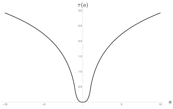
Figure 3.
The dynamics across the singularity is regular due to inverse volume corrections. In this picture, we show the function , defining the dynamical evolution across the singularity, in the case of Thiemann’s regularization of the inverse-area-operator.
The classical theory does not fix the evolution uniquely in this high curvature regime where quantum geometry effects cannot be neglected. Quantum geometry effects regularize the dynamics near the singularity; one way of seeing this is that the factor in the quantum evolution away from the singularity in (60) receives inverse volume quantum geometry corrections. As discussed in [35], these corrections are ambiguous (a fact that should not be surprising, given the expectation that the classical theory cannot guide us all the way to the deep UV in QFT). Instead of proposing one particular UV extension, as in the example shown where Thiemann regularization was used, one might simply keep all possibilities open and assume that the corresponding operator is regularized in the relevant region by some arbitrary function . In regions where , the quantum evolution leads to semiclassical equations that match exactly Einstein’s equations in the KS sector (more details in Section 3.6).
3.6. Dynamics of Semiclassical States and Tunneling across the Singularity
Let us first consider the vacuum case. This case is important because it should correspond to the Schrwarzschild interior in the region (or ). The dynamical evolution (65) becomes
In the representation, the previous equation simply reads
i.e., a simple translation in momentum space. Such dynamical evolution in a implies in an obvious manner that semiclassical states peaked at classical values at area with some given fluctuations will be simply evolved into the translated state with the very same fluctuation properties peaked at at area a. This is a remarkable property of the quantum system: independently of the quantum gravity effects encoded in the precise form of , expectation values satisfy well-defined effective dynamical equations which are exact (not an approximation), and semiclassical states are not spread by the dynamical evolution (as in the simple case of the harmonic oscillator). Notice that the validity of effective dynamical equations in the context of black hole models have remained a conjecture in other formulations [41].
In regions where , the previous evolution gives
From the definitions (30), we have that and . The constraint (25) gives us and the metric becomes
which corresponds to the Schrwarzschild solution with the two Dirac observables M and given in terms of the initial conditions by
When quantum inverse volume corrections are taken into account, then the quantum evolution is perfectly well-defined across the classical singularity. The evolution of the mean values of a semiclassical state is also well-defined and given by
Such solutions can also be obtained from the Hamiltonian constraint, given that one replaces the operator with its quantum regularization (effective equations are in this sense exact). The metric for all values of but otherwise arbitrary becomes
Since the Thiemann regularization produces a near , we see that the previous metric is just given by a two dimensional Minkowski metric fibrated with two dimensional sphere with time-dependent radius r. The shrinking of the spheres leads to a singularity at , where the spheres collapse and the spacetime geometry (as described by the effective line element) becomes a two-dimensional flat one at the singularity in the a-t plane. Despite the singular nature of the effective metric, the fundamental quantum evolution is well-defined across the singularity.
In the presence of matter, the situation is a bit more involved due to the factor appearing in matter’s contribution to the Hamiltonian constraint (60). However, in the spirit of applying this analysis to macroscopic black holes and modeling the dynamics of a weak scalar excitation (a Hawking particle) falling into the singularity, it is natural to focus on semiclassical states (Gaussian) peaked on values such that with fluctuations . As in the vacuum case , i.e., , is a constant of motion and its spread, . The dynamics of the conjugate variable (the mean value of the variable ) can be evaluated using stationary phase methods, and the result is
which can be seen to correspond to the classical solutions found in Section 2.3. Notice that, as expected from the form of the matter coupling, there are here quantum corrections characterized by terms proportional to . The spread in the variable is not time-independent if we take into account higher order corrections, namely,
The previous equations are derived assuming that the scalar field is in an eigenstate of the momentum . This is an idealization that simplifies the analysis of the dynamical evolution of the geometry. Similarly, if we assume that the geometry state was in an eigenstate of m, then we can easily analyze the dynamics of the scalar field assuming that it is initially in a Gaussian semiclassical state picked about and . In accordance with the classical solutions, we get
One way to quickly derive these equations by inspection is to realize that the Hamiltonian constraint (33) is that of a nonrelativistic point particle with mass proportional to our geometric variable m evolving in . Note that (77) implies that the back-reaction of the scalar field enters only through a simple modification of the exponential conformal factor in front of the 2-metric in the a-t ‘plane’ in Equation (76).
Unlike the geometry degrees of freedom, the fluctuations in the scalar field grow as one approaches the would-be singularity: for a given geometry semiclassical state picked around the mass M, the spread of the scalar field in an initial eigenstate of at area a grows to a maximum value close to the would-be singularity such that
which are small in the interior if we take , as expected from the appearance of in the fundamental commutation relations [42]. Note that, if we take into account inverse volume corrections of the type suggested by LQG (see Figure 3), the scalar field reaches a critical point at where its area velocity vanishes.
3.7. The Mass Operator (in the Vacuum Case)
In this section, we concentrate on the vacuum case for simplicity, as the mass can be directly read off the form of the metric, in this case via a simple comparison with the classical Schwarzschild solution. In this case, the result is
where we used the vacuum solution (16) (in its approximation) and (30). It is easy to verify that the previous is indeed a Dirac observable by showing that it commutes with Hamiltonian constraint (33). Its nonlinear dependence on the basic variables anticipates factor-ordering ambiguities when it comes to promoting the mass to a quantum operator. Here, we focus on the choice
where . The eigenstates equation
turns into the differential equation
If we expand the eigenstate in the basis,
where the sum runs over the discrete lattice as defined in (56) when introducing the dynamical constraint (60). This differential eigenvalue equation is solved by
where is a Bessel function. One can explicitly verify that the quantum dynamics (60) preserves the eigenstates by explicitly showing that the evolution between arbitrary lattice points sends the wave function of the eigenstate at the lattice point to the lattice point (as expected for a Dirac observable); or equivalently, the eigenstates of the mass are physical states solving (60). Explicitly,
Now, the evolution across requires inverse volume corrections, which modifies the previous dynamical law by replacing . The mass Dirac observable still exists once inverse volume corrections are turned on. It corresponds to the modification of (82) via the substitution . Eigenstates are also obtained by the same substitution in (86) and satisfy the expected Dirac observable condition (which now holds for lattice points at different sides across the singularity)
When supported on the same lattice, one can show that they satisfy the orthogonality relation
where the inner product is computed with the physical inner product (62). Thus, the spectrum of the mass operator is continuous. It was argued in the context of the full LQG theory in [28,43,44] that the eigenspaces of the mass should be infinitely degenerate due to the underlying discrete structure of the fundamental theory and the existence of defects that would not be registered in the ADM mass operator. Interestingly, the conjectured property is illustrated explicitly in our simple toy model, as for the eigenvectors (85) for a given eigenvalue, M, there are infinitely many and labeled by a continuum parameter. More precisely, they are associated with wave functions of the form (86) supported on lattices with different values of . Thus, eigenstates of the mass should then be denoted with orthogonality relation
where is the Kronecker delta symbol. The existence of such a large degeneracy is a generic feature of the polymer representation. Even when this is a toy model of quantum gravity, this feature is likely to reflect a basic property of the representation of the algebra of observables in the full LQG context. Here, we are showing that the mass operator is hugely degenerate, suggesting that the usual assumption of the uniqueness of the vacuum in background-dependent treatments of quantum field theory might fail in a full loop quantum gravity context.
Alternative factor orderings of the quantum operator M could be treated similarly (some simple choices lead to slightly different eigenvectors written also in terms of Bessel functions). Such an ambiguity is not relevant for our purposes (and it does not change the key fact that the spectrum of M is infinitely degenerate), as the aim of the model is not to construct any quantitative physical prediction but rather to use it as a toy model to investigate possibly sufficiently generic features that could actually survive in the full theory. The large degeneracy of the mass spectrum is, in our view, an interesting example of one such feature.
4. Discussion
We have shown that test-field solutions of the Klein–Gordon equation with zero angular momentum behave like solutions of the KS symmetry-reduced model in the deep interior region defined in terms of the background Schwarzschild spacetime. This implies that spherically symmetric scalar matter falling into a spherical black hole can be modeled by the KS solutions near the singularity. Despite the expected limitations of symmetry-reduced models in capturing the full physics in the UV regime, the model includes back-reaction of the scalar matter. Focusing on the deep interior region and using perturbation theory in , we show that it is possible to interpret the solutions of KS with matter as Schwarzschild solutions with matter excitations falling towards the singularity (this interpretation is not global but is shown to be correct in the deep interior region). The Hamiltonian dynamics simplifies considerably in that regime, becoming tractable both at the classical level and the quantum level. Perturbation theory applies (we have shown) to the situation involving Hawking particles falling into the singularity.
In close analogy to LQG, we define a quantization of the system describing the deep interior region, where the area of the r=constant spheres has a discrete spectrum. This leads to the polymer representation of the area of the orbits of the rotation group and its conjugate momentum that allows for a well-defined quantum evolution across the singularity if one introduces customary ’inverse-volume’ corrections to the quantum scalar constraint. The Hamiltonian constraint admits a simple geometric interpretation in the to-be-polymerized sector due to the linearity of the Hamiltonian constraint in the momentum variable conjugated to the area of the r=constant spheres. The geometric nature of the action of the classical constraint allows for the introduction of a unique polymerization prescription respecting this action at the quantum level. This reduces the ambiguity usually associated with the procedure of quantization of the dynamical constraints for reasons that resonate with the ones that lead to similar advantages in the full theory [38]. Remarkably, the dynamics is exactly solvable at the quantum level. In the vacuum case, the mass operator is a Dirac observable that we quantize and whose spectrum is given explicitly. Semiclassical states dynamics leads to effective evolution equations that can be characterized exactly in the vacuum case and using suitable stationary phase approximations in the case where matter is present. These effective equations coincide with Einsteins equations in regions where the inverse volume corrections can be neglected.
An important formal aspect of the model is that it presents a concrete example of violation of the ’unicity of the vacuum’ assumption that permeates discussions of Hawking’s information puzzle for over 40 years. In loop quantum gravity, the discrete structure of the theory at the Planck scale suggests that a given (macroscopic) ADM mass configuration need not correspond to a unique quantum state. High degeneracy due to the contribution of microscopic degrees of freedom is expected but hard to prove at the present stage. This leads to a certain degree of disagreement on the status of such statements in the field at large. Although a key instance where such degeneracy is accepted with little controversy is in the loop quantum gravity models designed to calculate black hole entropy (for reviews and references see [45,46]) where the statistical origin of the entropy lies precisely in the large multiplicity of underlying microscopic states. Our simple model might still be too simple to represent definite evidence in this direction. Nevertheless, the results of Section 3.7 do provide a toy model to eventually study the implications of the large degeneracy of the mass spectrum in discussion of the fate of information in black hole evaporation.
The model we introduce here is simple and workable. We hope it could provide potentially useful insights in dealing with qualitative questions concerning black hole evaporation. The investigation of these interesting possibilities is left for the future.
Author Contributions
Investigation, A.P., S.R., S.V.; Data curation, A.P., S.R., S.V.; Writing—original draft preparation, A.P., S.R., S.V.; writing—review and editing, A.P., S.R., S.V. All authors have read and agreed to the published version of the manuscript.
Funding
This research received no external funding.
Institutional Review Board Statement
Not applicable.
Informed Consent Statement
Not applicable.
Data Availability Statement
Not applicable.
Acknowledgments
We thank the interaction with Simone Speziale for valuable insights and specially for discussion on the Hamiltonian analysis of the system.
Conflicts of Interest
The authors declare no conflict of interest.
Note
| 1 | The Hawking effect is a quantum process, and the relavant state describing it is a quantum state that corresponds to the vacuum in the far past idealized by . Such state can be viewed in the interior as a superposition of particles. Actual particles appear inside in the hypothetical situation of the detection of a partner at , which according to the standard interpretation of quantum mechanics, will produce a collapse of the vacuum to a new state containing an actual particle falling into the black hole. The situation after such collapse is the semiclassical situation that we model here with our classical language. A precise description of such a situation in quantum terms is a question that can only be addressed in a full theory of quantum gravity. We argue here that our solvable model goes a humble step in that direction. |
References
- Ashtekar, A. New Variables for Classical and Quantum Gravity. Phys. Rev. Lett. 1986, 57, 2244–2247. [Google Scholar] [CrossRef]
- Ashtekar, A. New Hamiltonian Formulation of General Relativity. Phys. Rev. D 1987, 36, 1587–1602. [Google Scholar] [CrossRef]
- Perez, A. Introduction to loop quantum gravity and spin foams. In Proceedings of the 2nd International Conference on Fundamental Interactions (ICFI 2004), Espirito Santo, Brazil, 6–12 June 2004. [Google Scholar]
- Ashtekar, A.; Lewandowski, J. Background independent quantum gravity: A Status report. Class. Quant. Grav. 2004, 21, R53. [Google Scholar] [CrossRef]
- Rovelli, C. Quantum Gravity; Cambridge Monographs on Mathematical Physics; Cambridge University Press: Cambridge, UK, 2004. [Google Scholar]
- Thiemann, T. Modern Canonical Quantum General Relativity; Cambridge Monographs on Mathematical Physics; Cambridge University Press: Cambridge, UK, 2007. [Google Scholar]
- Agullo, I.; Singh, P. Loop Quantum Cosmology; WSP: Montreal, QC, Canada, 2017; pp. 183–240. [Google Scholar]
- Bojowald, M. Absence of singularity in loop quantum cosmology. Phys. Rev. Lett. 2001, 86, 5227–5230. [Google Scholar] [CrossRef]
- Bojowald, M. Loop quantum cosmology. Living Rev. Rel. 2005, 8, 11. [Google Scholar] [CrossRef] [PubMed]
- Ashtekar, A.; Bojowald, M.; Lewandowski, J. Mathematical structure of loop quantum cosmology. Adv. Theor. Math. Phys. 2003, 7, 233–268. [Google Scholar] [CrossRef]
- Ashtekar, A.; Singh, P. Loop Quantum Cosmology: A Status Report. Class. Quant. Grav. 2011, 28, 213001. [Google Scholar] [CrossRef]
- Taveras, V. Corrections to the Friedmann Equations from LQG for a Universe with a Free Scalar Field. Phys. Rev. D 2008, 78, 064072. [Google Scholar] [CrossRef]
- Modesto, L. Disappearance of black hole singularity in quantum gravity. Phys. Rev. 2004, D70, 124009. [Google Scholar] [CrossRef]
- Ashtekar, A.; Bojowald, M. Quantum geometry and the Schwarzschild singularity. Class. Quant. Grav. 2006, 23, 391–411. [Google Scholar] [CrossRef]
- Modesto, L. Loop quantum black hole. Class. Quant. Grav. 2006, 23, 5587–5602. [Google Scholar] [CrossRef]
- Gambini, R.; Pullin, J. Loop quantization of the Schwarzschild black hole. Phys. Rev. Lett. 2013, 110, 211301. [Google Scholar] [CrossRef]
- Gambini, R.; Pullin, J. Black holes in loop quantum gravity: The Complete space-time. Phys. Rev. Lett. 2008, 101, 161301. [Google Scholar] [CrossRef]
- Gambini, R.; Olmedo, J.; Pullin, J. Quantum black holes in Loop Quantum Gravity. Class. Quant. Grav. 2014, 31, 095009. [Google Scholar] [CrossRef]
- Gambini, R.; Pullin, J. Quantum shells in a quantum space-time. Class. Quant. Grav. 2015, 32, 035003. [Google Scholar] [CrossRef]
- Ashtekar, A.; Olmedo, J.; Singh, P. Quantum Transfiguration of Kruskal Black Holes. Phys. Rev. Lett. 2018, 121, 241301. [Google Scholar] [CrossRef]
- Nicolini, P.; Spallucci, E.; Wondrak, M.F. Quantum Corrected Black Holes from String T-Duality. Phys. Lett. B 2019, 797, 134888. [Google Scholar] [CrossRef]
- Koch, B.; Saueressig, F. Black holes within Asymptotic Safety. Int. J. Mod. Phys. A 2014, 29, 1430011. [Google Scholar] [CrossRef]
- Saueressig, F.; Alkofer, N.; D’Odorico, G.; Vidotto, F. Black holes in Asymptotically Safe Gravity. PoS 2016, FFP14, 174. [Google Scholar]
- Bardeen, J.M. Non-singular general-relativistic gravitational collapse. In Proceedings of the International Conference GR5, Tbilisi, GA, USA, 9–13 September 1968; Volume 174, p. 174. [Google Scholar]
- Hayward, S.A. Formation and evaporation of regular black holes. Phys. Rev. Lett. 2006, 96, 031103. [Google Scholar] [CrossRef]
- Lorenzo, T.D.; Pacilio, C.; Rovelli, C.; Speziale, S. On the Effective Metric of a Planck Star. Gen. Rel. Grav. 2015, 47, 41. [Google Scholar] [CrossRef]
- Frolov, V.P. Notes on nonsingular models of black holes. Phys. Rev. D 2016, 94, 104056. [Google Scholar] [CrossRef]
- Perez, A.; Sudarsky, D. A dialog on the fate of information in black hole evaporation. arXiv 2022, arXiv:2205.08469. [Google Scholar] [CrossRef]
- Kantowski, R.; Sachs, R.K. Some spatially homogeneous anisotropic relativistic cosmological models. J. Math. Phys. 1966, 7, 443–446. [Google Scholar] [CrossRef]
- Ashtekar, A.; del Río, A. Probing cosmological singularities with quantum fields: Open and closed FLRW universes. Phys. Rev. D 2022, 106, 085003. [Google Scholar] [CrossRef]
- Ashtekar, A.; del Río, A.; Schneider, M. Space-like Singularities of General Relativity: A Phantom menace? Gen. Rel. Grav. 2022, 54, 45. [Google Scholar] [CrossRef]
- Xanthopoulos, B.C.; Zannias, T. Kantowski–Sachs metrics with source: A massless scalar field. J. Math. Phys. 1992, 33, 1415–1419. [Google Scholar] [CrossRef]
- Page, D.N. Particle Emission Rates from a Black Hole: Massless Particles from an Uncharged, Nonrotating Hole. Phys. Rev. D 1976, 13, 198–206. [Google Scholar] [CrossRef]
- Poisson, E.; Israel, W. Internal structure of black holes. Phys. Rev. D 1990, 41, 1796–1809. [Google Scholar] [CrossRef]
- Amadei, L.; Perez, A.; Ribisi, S. The landscape of polymer quantum cosmology. arXiv 2022, arXiv:2203.07044. [Google Scholar]
- Perez, A. On the regularization ambiguities in loop quantum gravity. Phys. Rev. D 2006, 73, 044007. [Google Scholar] [CrossRef]
- Münch, J.; Perez, A.; Speziale, S.; Viollet, S. Generic features of a polymer quantum black hole. arXiv 2022, arXiv:2212.06708. [Google Scholar]
- Ashtekar, A.; Varadarajan, M. Gravitational Dynamics—A Novel Shift in the Hamiltonian Paradigm. Universe 2021, 7, 13. [Google Scholar] [CrossRef]
- Varadarajan, M. Anomaly free quantum dynamics for Euclidean LQG. arXiv 2022, arXiv:2205.10779. [Google Scholar]
- Varadarajan, M.; Perez, A. Public and private discussion. In Proceedings of the LOOPs 22 Conference, Lyon, France, 18–22 July 2022. [Google Scholar]
- Ashtekar, A.; Olmedo, J.; Singh, P. Quantum extension of the Kruskal spacetime. Phys. Rev. D 2018, 98, 126003. [Google Scholar] [CrossRef]
- Rovelli, C.; Wilson-Ewing, E. Why are the effective equations of loop quantum cosmology so accurate? Phys. Rev. D 2014, 90, 023538. [Google Scholar] [CrossRef]
- Perez, A. No firewalls in quantum gravity: The role of discreteness of quantum geometry in resolving the information loss paradox. Class. Quant. Grav. 2015, 32, 084001. [Google Scholar] [CrossRef]
- Amadei, L.; Liu, H.; Perez, A. Unitarity and information in quantum gravity: A simple example. Front. Astron. Space Sci. 2021, 8, 46. [Google Scholar] [CrossRef]
- Barbero G, J.F.; Perez, A. Quantum Geometry and Black Holes; WSP: Montreal, QC, Canada, 2017; pp. 241–279. [Google Scholar]
- Perez, A. Black Holes in Loop Quantum Gravity. Rept. Prog. Phys. 2017, 80, 126901. [Google Scholar] [CrossRef]


Disclaimer/Publisher’s Note: The statements, opinions and data contained in all publications are solely those of the individual author(s) and contributor(s) and not of MDPI and/or the editor(s). MDPI and/or the editor(s) disclaim responsibility for any injury to people or property resulting from any ideas, methods, instructions or products referred to in the content. |
© 2023 by the authors. Licensee MDPI, Basel, Switzerland. This article is an open access article distributed under the terms and conditions of the Creative Commons Attribution (CC BY) license (https://creativecommons.org/licenses/by/4.0/).