Perturbations in Bianchi-V Spacetimes with Varying Λ, G and Viscous Fluids

Abstract

As a follow-up of a recent article in which we investigated the cosmological background expansion history of the universe in Bianchi type-V cosmological models with bulk viscous fluid and evolving cosmological $\Lambda$ and Newtonian G parameters, we study the evolution of the cosmological perturbations in the current work. In particular, we analyse the evolution of the viscous matter over-density that leads to formation of large-scale structures in the Bianchi-V model, and compare the results with standard $\Lambda$CDM solutions. Our results suggest that introducing viscous fluid in the background described by Bianchi-V geometry with evolving $\Lambda$ and G amplifies the structure-growth rate.

1. Introduction

The recent cosmological data from the strong redshift of type Ia supernovae and changes in the cosmic microwave background power spectrum (CMB) [1,2,3,4] suggest that the universe is currently undergoing a late-time accelerating expansion. From the standard model of cosmology point of view, the cosmic acceleration is attributed to dark energy (DE). It is thought to be a type of cosmic matter with a negative density. Cosmological data have shown that it makes up around $70\%$ of the universe’s total energy density. With its nature largely unknown, one of the candidates put forth as a candidate source for DE is Einstein’s cosmological parameter $\Lambda$. Furthermore, one of the several possible scenarios in which $\Lambda$ is considered a good DE candidate is as a function of time, instead of the usual consideration of it being a constant, because its cosmological effect seems to have evolved with time from being small in the early stages of the universe to its present dominance. Furthermore, because Newton’s gravitational force was the only dominant force in the early moments of the universe and the value of Newton’s constant G is very small in comparison to what it was in the past, it is more appropriate and necessary to choose Newton’s constant as a function of time alongside Einstein’s constant.

Based on this discussion, there are two conceivable strategies for considering the coupling of G and $\Lambda$ to be varying functions; these are modifications at the level of the equation of motion, and modifications at the level of the action. Regrading the modifications at the level of the action, both G and $\Lambda$ will be coupled to the matter of “scale-dependent couplings” in the Einstein–Hilbert action. Such a coupling will induce an additional contribution $△t_{ij}=G_k(g_{ij}\square -{\nabla }_i{\nabla }_i)G_k^{-1}$ to the stress energy tensor in field equations. Cosmological aspects of this approach, such as the evolution of density perturbations in the context of asymptotically safe gravity or scale-dependent gravity, where both the cosmological constant and the Newtonian running constants are permitted to change over time, have been examined by numerous researchers [5,6,7,8,9,10].

Bianchi models are primarily motivated by Bianchi’s work [11,12], and are non-standard cosmological models that are homogeneous and non-isotropic in general. Further motivated by Dirac’s hypothesis [13] on the evolution of the fundamental ‘constants’, in this case $\Lambda$ and G, Bianchi-type cosmological models with varying cosmological and Newtonian constants have recently been studied by a number of researchers [14,15,16,17,18,19,20,21]. In this work [22], for instance, a Bianchi type-V viscous fluid cosmological model for barotropic fluid distribution with a variable cosmological term was investigated, and it was shown that cosmic isotropization occurs asymptotically, with acceleration induced by the presence of shear viscosity. Furthermore, Singh and others [23,24] demonstrated bulk viscous Bianchi type-V cosmological models with a time-dependent cosmological term. By assuming that the shear scalar is proportional to the volume expansion, and the bulk viscosity coefficient is a power function of the energy density or volume expansion, exact solutions to Einstein’s field equations are achieved.

In a recent article [25], we investigated the viability of the Bianchi type-Vcosmological model, filled with bulk viscous universe and time-dependent cosmological parameter $\Lambda$ and Newtonian gravitational parameter G. We showed that such a model can adequately describe a universe that starts off with a negative cosmological term, dominated by normal matter in a decelerated background, that eventually becomes dark energy-dominated (and hence accelerated) spacetime at late times, in concordance with current observations. This follow-up work aims to tackle the nature of large-scale structure formation through cosmological perturbations around the Bianchi type-V spacetime background which, to our knowledge, has not been considered in any existing literature. In particular, we follow the $1+3$ covariant formalism of cosmological perturbations to derive the evolution equations governing the perturbations of the matter energy density, expansion and shear perturbations. We then couple these equations with the background field equations derived in P1 to evaluate the rate of structure formation in the Bianchi-V model under investigation.

The rest of the work is organised as follows: Section 2 gives a quick recap of the the Bianchi type-V background cosmological model. The perturbations around the Bianchi type-V background will be presented in Section 3. Section 4 will offer several cosmological models based on the selection of time-varying shear and bulk viscosity. Finally, we bring the article to a close with our conclusions in Section 5.

2. Background Field Equations

In orthogonal space and time coordinates, the Bianchi type-V metric is given by the following formula:

$$d{s}^2=d{t}^2-A^{2}d{x}^2-e^{2Kx}[B^{2}d{y}^2+C^{2}d{z}^2].$$

(1)

Here the metric coefficients A, B and C are functions of time, and K is constant that is related to the curvature of spatial part. Assuming that a viscous fluid fills the universe, the energy momentum tensor shown below represents the fluid’s distribution in space:

$$T_{ij}=(\rho +\overline{p})u_i{u}_j+\overline{p}{g}_{ij}-2\eta {\sigma }_{ij},$$

(2)

where $\rho$ is matter-energy density, $\overline{p}$ is the effective pressure, $u^i=(u^1,u^2,u^3,u^4)=(0,0,0,1)$ is four-velocity vector of the cosmic fluid which is normalized as $u_i{u}^i=-1$, ${\sigma }_{ij}$ is the shear tensor and $\eta >0$ is the coefficient of shear viscosity. The effective pressure $\overline{p}$ is defined in terms of the isotropic pressure p and the coefficients of viscosity as

$$\begin{array}{c}\hfill \overline{p}=p-\xi {\nabla }^i{u}_i=p-\left(3\xi -2\eta \right)H.\end{array}$$

(3)

where $\xi >0$ is the coefficient of bulk viscosity and H is the Hubble parameter. Now, we assume that the fluid has the following linear equation of state (EoS)

$$p=w\rho ,$$

where $-1\le w\le 1$ is the EoS parameter. The shear tensor is defined as

$$\begin{array}{c}\hfill {\sigma }_{ij}=h_j^k{\nabla }_k{u}_i+h_i^k{\nabla }_k{\dot{u}}_j-\frac{1}{3}\theta h_{ij},\end{array}$$

(4)

where $h_{ij}=g_{ij}+u_i{u}_j$ is the projection tensor and $\theta$ is the expansion scalar.

The field equations of the theory of general relativity with cosmological constant $\Lambda$ are

$$R_{ij}-\frac{1}{2}{g}_{ij}R=-\kappa G{T}_{ij}+\Lambda g_{ij}.$$

(5)

where $c=1$ is taken, $\kappa \equiv 8\pi$, G is the Newtonian gravitational constant, $g_{ij}$ is the metric tensor of the 4-dimensional space-time, $R_{ij}$ is the Ricci tensor, and R is the Ricci scalar. Here, in this study, we assume that both G and $\Lambda$ are no longer constants, but are functions of time.

Einstein field equations (EFEs) in (5) for the Bianchi type-V universe filled with a viscous fluid distribution are obtained as follows:

$$\begin{array}{cc}\hfill -\frac{\ddot{B}}{B}-\frac{\ddot{C}}{C}-\frac{\dot{B}}{B}\frac{\dot{C}}{C}+\frac{K^2}{A^2}+2\eta \kappa G\frac{\dot{A}}{A}& =\kappa G\left[p-\left(\xi -\frac{2}{3}\eta \right)\theta \right]-\Lambda ,\hfill \end{array}$$

(6)

$$\begin{array}{cc}\hfill -\frac{\ddot{A}}{A}-\frac{\ddot{C}}{C}-\frac{\dot{A}}{A}\frac{\dot{C}}{C}+\frac{K^2}{A^2}+2\eta \kappa G\frac{\dot{B}}{B}& =\kappa G\left[p-\left(\xi -\frac{2}{3}\eta \right)\theta \right]-\Lambda ,\hfill \end{array}$$

(7)

$$\begin{array}{cc}\hfill -\frac{\ddot{A}}{A}-\frac{\ddot{B}}{B}-\frac{\dot{A}}{A}\frac{\dot{B}}{B}+\frac{K^2}{A^2}+2\eta \kappa G\frac{\dot{C}}{C}& =\kappa G\left[p-\left(\xi -\frac{2}{3}\eta \right)\theta \right]-\Lambda ,\hfill \end{array}$$

(8)

$$\begin{array}{cc}\hfill \frac{\dot{A}}{A}\frac{\dot{B}}{B}+\frac{\dot{A}}{A}\frac{\dot{C}}{C}+\frac{\dot{B}}{B}\frac{\dot{C}}{C}-\frac{3K^2}{A^2}& =\kappa G\rho +\Lambda ,\hfill \end{array}$$

(9)

$$\begin{array}{cc}\hfill -2\frac{\dot{A}}{A}+\frac{\dot{B}}{B}+\frac{\dot{C}}{C}& =0.\hfill \end{array}$$

(10)

Here, an overdot represents a derivative with respect to cosmic time t.

The time dependence of G and $\Lambda$, together with consideration of the covariant derivative of the energy momentum tensor (2) involving viscosity, leads to the conservation equation of the form

$$\begin{array}{c}\hfill \kappa G\left[\dot{\rho }+(\overline{p}+\rho )\left(\frac{\dot{A}}{A}+\frac{\dot{B}}{B}+\frac{\dot{C}}{C}\right)\right]+\kappa \rho \dot{G}+\dot{\Lambda }-4\kappa G\eta {\sigma }^2=0.\end{array}$$

(11)

Assuming that the total matter content of the universe is conserved, this conservation equation can be thought of as two different equations; using Equation (3), these two independent equations are written as follows:

$$\begin{array}{ccc}& & \dot{\rho }+3H\left[p+\rho -(3\xi -2\eta )H\right]-4\eta {\sigma }^2=0,\hfill \end{array}$$

(12)

$$\begin{array}{ccc}& & \kappa \rho \dot{G}+\dot{\Lambda }=0.\hfill \end{array}$$

(13)

Here, the shear scalar $\sigma$, ${\sigma }_0$ being a constant that is related to the anisotropy of the universe, is given by

$$\begin{array}{c}\hfill {\sigma }^2=\frac{1}{2}{\sigma }_{ij}{\sigma }^{ij}=\frac{{\sigma }_0^2}{a^6},\end{array}$$

(14)

and definition of the mean Hubble parameter is used for the term $\left(\frac{\dot{A}}{A}+\frac{\dot{B}}{B}+\frac{\dot{C}}{C}\right)$. In Bianchi type space-times, the concept of the mean Hubble parameter is based on the definitions of a spatial volume V and a mean scale factor a given by

$$\begin{array}{c}\hfill V=a^3=\sqrt{|-g_{ij}|}=ABC.\end{array}$$

(15)

According to Equation (15), the average Hubble parameter H and the average deceleration parameter q are defined as

$$H\equiv \frac{\dot{a}}{a}=\frac{1}{3}\left(H_x+H_y+H_z\right),q\equiv -\frac{a\ddot{a}}{{\dot{a}}^2}=-\frac{\dot{H}}{H^2}-1,$$

(16)

where $H_x,H_y$ and $H_z$ are the directional Hubble parameters along x, y and z directions, respectively. For a Bianchi type-V universe, the directional Hubble parameters are $H_x=\frac{\dot{A}}{A},H_y=\frac{\dot{B}}{B}$ and $H_z=\frac{\dot{C}}{C}$. The components of the shear tensor ${\sigma }_{ij}$ for the Bianchi type-V model given by Equation (1) are obtained as

$${\sigma }_{11}=H_x-H,{\sigma }_{22}=H_y-H,{\sigma }_{33}=H_z-H,{\sigma }_{44}=0,$$

(17)

and the shear scalar $\sigma$ as

$${\sigma }^2=\frac{1}{6}\left[{\left(\frac{\dot{A}}{A}-\frac{\dot{B}}{B}\right)}^2+{\left(\frac{\dot{B}}{B}-\frac{\dot{C}}{C}\right)}^2+{\left(\frac{\dot{C}}{C}-\frac{\dot{A}}{A}\right)}^2\right].$$

(18)

The field equations given in Equations (6)–(10) can be written in terms of H, q and $\sigma$ as

$$\begin{array}{ccc}& & \kappa G\overline{p}-\Lambda =H^2(2q-1)-{\sigma }^2+\frac{K^2}{A^2},\hfill \end{array}$$

(19)

$$\begin{array}{ccc}& & \kappa G\rho +\Lambda =3H^2-{\sigma }^2-\frac{3K^2}{A^2}.\hfill \end{array}$$

(20)

Equations (19) and (20) are dubbed as generalized Friedmann equations for a Bianchi type-V universe filled with the viscous fluid. The generalized Raychaudhuri equation for this model is obtained as

$$\begin{array}{c}\hfill \dot{H}+3H^2-\frac{2K^2}{a^2}-\Lambda +\frac{\kappa G}{2}(p-\rho )-\kappa G\left(\frac{3\xi }{2}-\eta \right)H=0.\end{array}$$

(21)

It is impossible to solve this equation as it is because of the unknown variables $\eta ,\xi ,a,G,\Lambda ,p$ and $\rho$. To find the solution by introducing extra information in the form of initial conditions and a constraint, we consider the following form of the Friedmann Equation (20) divided by $3H^2$:

$$1={\Omega }_m+{\Omega }_{\Lambda }+{\Omega }_{\sigma }+{\Omega }_{\chi },$$

(22)

where

$$\begin{array}{c}\hfill {\Omega }_m\equiv \frac{\kappa G{\rho }_m}{3H^2},{\Omega }_{\Lambda }\equiv \frac{\kappa G{\rho }_{\Lambda }}{3H^2},{\Omega }_{\sigma }\equiv \frac{{\sigma }^2}{3H^2},{\Omega }_{\chi }\equiv \frac{K^2}{H^2{a}^2}\end{array}$$

(23)

are called density parameters. The current values of these dimensionless density parameters are given in terms of the current values of the quantities that describe them, as

$$\begin{array}{c}\hfill {\Omega }_{m_0}=\frac{\kappa G_0{\rho }_{m_0}}{3H_0^2},{\Omega }_{{\Lambda }_0}=\frac{\kappa G_0{\rho }_{{\Lambda }_0}}{3H_0^2},{\Omega }_{{\sigma }_0}=\frac{{\sigma }_0^2}{3H_0^2},{\Omega }_{{\chi }_0}=\frac{K^2}{H_0^2{a}_0^2},\end{array}$$

(24)

For the linear barotropic fluid, the conservation Equations (12) and (13) are obtained in terms of the dimensionless density parameters (23) as follows:

$$\begin{array}{cc}\hfill {\dot{\Omega }}_m& +\left(2\frac{\dot{H}}{H}-\frac{\dot{G}}{G}\right){\Omega }_m+3H(1+w_m){\Omega }_m-\kappa G\left[(3\xi -2\eta )+4\eta {\Omega }_{\sigma }\right]=0,\hfill \end{array}$$

(25)

$$\begin{array}{cc}\hfill {\dot{\Omega }}_{\Lambda }& +2\frac{\dot{H}}{H}{\Omega }_{\Lambda }+\frac{\dot{G}}{G}{\Omega }_m=0.\hfill \end{array}$$

(26)

In order to solve the different ${\Omega }_i$’s, one more equation is necessary besides the evolution Equations (25) and (26), together with the constraint (22). Therefore, we use the following additional evolution equations for the fractional energy density:

$$\begin{array}{ccc}\hfill & & {\dot{\Omega }}_{\chi }+2\left(H+\frac{\dot{H}}{H}\right){\Omega }_{\chi }=0,\hfill \end{array}$$

(27)

$$\begin{array}{ccc}& & {\dot{\Omega }}_{\sigma }+\left(6H+2\frac{\dot{H}}{H}\right){\Omega }_{\sigma }=0.\hfill \end{array}$$

(28)

Now, we see that our model consists of only five differential equations, such as (6)–(10), (12) and (13), but contains six unknowns (H, ${\Omega }_m$, ${\Omega }_{\Lambda }$, ${\Omega }_{\chi }$, ${\Omega }_{\sigma }$ and G). To complete this system of equations, we need an extra equation or assumption. To provide this necessity, we adopt the assumption

$$\begin{array}{c}\hfill G\left(t\right)=G_0{a}^{\delta }\end{array}$$

(29)

in accordance with Dirac’s ansatz, which states that the gravitational constant G must decrease with time. Here, $\delta =-1/60$ is a constant obtained from observational constraints [26] which is in a good agreement with results of [27].

Now, to numerically integrate our equations and see if/how the results compare with those of the $\Lambda CDM$ model, we express the evolution equations of our model in redshift (z) space using the transformation formula:

$$\begin{array}{cc}\hfill \dot{f}=\frac{df}{dt}& =\frac{df}{dz}\frac{dz}{da}\frac{da}{dt}=-(1+z)H{f}^{\prime }\hfill \end{array}$$

(30)

where f is arbitrary function of time t, and we introduce the following dimensionless parameters

$$h\equiv \frac{H}{H_0},a=\frac{1}{(1+z)},\xi =\alpha H_0{({\rho }_m/{\rho }_{m0})}^n,and\eta =\beta H.$$

Here $\alpha$, $\beta$ and $0\le n\le \frac{1}{2}$ are dimensionless constants. For more details about $\xi \left(t\right)$ being a simple power function of the energy density see [28,29,30,31]. Then, the evolution Equations (21), (25)–(28) become a completely dimensionless system in redshift space as follows

$$\begin{array}{cc}\hfill h^{\prime }& =\frac{h}{(1+z)}\left[3-2{\Omega }_{\chi }-3{\Omega }_{\Lambda }-\frac{3}{2}(1-w_m){\Omega }_m\right]-\frac{\kappa G_0}{{(1+z)}^{1+\delta }}\left[\frac{3\alpha }{2}{\left(\frac{h^2{\Omega }_m{(1+z)}^{\delta }}{{\Omega }_{m0}}\right)}^n-\beta h\right]\hfill \end{array}$$

(31)

$$\begin{array}{cc}\hfill {\Omega }_m^{\prime }& =-\frac{2h^{\prime }}{h}{\Omega }_m+\frac{1}{1+z}\left(-\delta +3+3w_m\right){\Omega }_m-\frac{\kappa G_0}{{(1+z)}^{1+\delta }}\left[\frac{3\alpha }{h}{\left(\frac{h^2{\Omega }_m{(1+z)}^{\delta }}{{\Omega }_{m0}}\right)}^n-2\beta +4\beta {\Omega }_{\sigma }\right],\hfill \end{array}$$

(32)

$$\begin{array}{cc}\hfill {\Omega }_{\Lambda }^{\prime }& =-\frac{2h^{\prime }}{h}{\Omega }_{\Lambda }-\frac{\delta }{1+z}{\Omega }_m,\hfill \end{array}$$

(33)

$$\begin{array}{cc}\hfill {\Omega }_{\chi }^{\prime }& =-\frac{2h^{\prime }}{h}{\Omega }_{\chi }+\frac{2{\Omega }_{\chi }}{1+z},\hfill \end{array}$$

(34)

$$\begin{array}{cc}\hfill {\Omega }_{\sigma }^{\prime }& =-\frac{2h^{\prime }}{h}{\Omega }_{\sigma }+\frac{6{\Omega }_{\sigma }}{1+z},\hfill \end{array}$$

(35)

In what follows, Figure 1 and Figure 2 show the evolution of G and $\Lambda$ with redshift, and as expected, Figure 1 shows G decreasing with time (normalised to unity today), whereas Figure 2 shows $\Lambda$ increasing with time reaching its current (normalised) value of around 0.7. We also notice the evolution of the fractional matter density, which, as reported in [25], shows a local maximum at some recent redshift $z\sim 0.5$ and decreasing to its current value. This feature might suggest that the behaviour of expected matter decay is affected by viscosity in a non-trivial way for such models, and may be an interesting distinguishing feature worth looking out for in existing or future astronomical data, to confirm or rule out such models. Figure 3 shows the evolution of the fractional curvature and anisotropy parameters, with vanishingly small values today, as suggested by observations and the standard FLRW-based $\Lambda$CDM cosmology.

The background equations of this section will be used together with the perturbation equations derived in the following section to determine the rate of structure formation in our Bianchi type-V spacetime model with viscosity and evolving $\Lambda$ and G.

3. Perturbations

It is now a well-established fact that the universe is not perfectly smooth, but is full of large-scale structures (galaxies, clusters, superclusters, voids, etc.) seeded from primordial fluctuations. Cosmological perturbation theory provides the mechanism to explain how these small fluctuations grow and form the large-scale structures in the real, lumpy, universe. The actual procedure of perturbing can be done in two ways [32]: the metric-based approach, developed through the pioneering works of Lifshitz [33], Bardeen [34], and Kodama and Sasaki [35], and the covariant approach developed by Ehlers [36], Hawking [37], Olson [38], and Ellis and Bruni [39]. The first approach involves the foliation of the background spacetime with hypersurfaces and perturbing away from it. It is a non-local, linear theory which requires that the metric be specified from the start. Difficulty dealing with nonlinear effects and in handling the unphysical gauge modes that are inherent to the theory are the main disadvantages of this approach [39,40,41]. The covariant formalism, on the other hand, is a way of describing spacetime via covariantly defined variables with respect to a partial frame formalism such as the $1+3$ [39] or $1+1+2$ [42] spacetime decomposition techniques. It is a suitable method to describe physics and geometry using tensor quantities and relations valid in all coordinate systems. It is a local, covariant theory based on threading spacetimes with frames. This approach differs from the standard one in that it starts from the theory and reduces to linearities in a particular background. Nonlinearities can be accommodated, but the main advantage of this approach is that no unphysical gauge modes appear here.

Existing work in the study of cosmological dynamics universes filled with viscous fluid models with evolving $\Lambda$ and G focus, to the most part, on the background expansion history. To our knowledge, there has been, for example, no work on the large-scale structure formation scenarios of such viscous-fluid-filled Bianchi-V spacetimes. We will therefore attempt to close this gap by studying the perturbations of such spacetimes, as these perturbations are generally understood to be the seeds of the large-scale structures we see in the universe today (see [32] and references therein for more details). To do so, we start by defining the covariant and gauge-invariant gradient variables that describe perturbations in the matter energy density, expansion and shear, as per the $1+3$ covariant perturbation formalism [39,43,44]:

$$D_a\equiv \frac{a{\tilde{\nabla }}_a^{}\rho }{\rho },Z_a\equiv a{\tilde{\nabla }}_a^{}\Theta ,{\Sigma }_a\equiv a{\tilde{\nabla }}_a^{}\sigma .$$

(36)

These gradient variables evolve according to the following equations:

$$\begin{array}{ccc}& & {\dot{D}}_a-\left[w-\left(\xi -\frac{2\beta }{9}\Theta \right)\frac{\Theta }{\rho }+\frac{\left(n\xi \Theta -w\rho \right)(4\beta {\sigma }^2/3\rho )}{(1+w)\rho -\left(\xi -\frac{2\beta }{9}\Theta \right)\Theta }-\frac{4\beta {\sigma }^2}{3\rho }\right]\Theta D_a-Y_a\hfill \\ & & +\left[1+w-\left(\xi -\frac{2\beta }{9}\Theta \right)\frac{\Theta }{\rho }+\frac{\left(\xi -\frac{4\beta }{9}\Theta \right)(4\beta {\sigma }^2/3)}{(1+w)\rho -\left(\xi -\frac{2\beta }{9}\Theta \right)\Theta }\frac{\Theta }{\rho }-\frac{4\beta {\sigma }^2}{3\rho }\right]Z_a+\frac{8\beta }{3}\frac{\Theta }{\rho }\sigma {\Sigma }_a\hfill \\ & & +\left[1-\frac{\frac{4\beta {\sigma }^2}{3}}{(1+w)\rho -\left(\xi -\frac{2\beta }{9}\Theta \right)\Theta }\right]\frac{2\beta \Theta }{3\rho }{X}_a=0,\hfill \end{array}$$

(37)

$$\begin{array}{ccc}& & {\dot{Z}}_a+\left[\frac{2}{3}\Theta -\frac{3\kappa G}{2}\left(\xi -\frac{4\beta }{9}\Theta \right)-\frac{\left(\xi -4\beta /9\Theta \right)\dot{\Theta }}{(1+w)\rho -\left(\xi -2\beta /9\Theta \right)\Theta }\right]Z_a\hfill \\ & & -\frac{\left(\xi -4\beta /9\Theta \right)}{\rho +p-\left(\xi -2\beta /9\Theta \right)\Theta }{\tilde{\nabla }}^{}{}^2{Z}_a\hfill \\ & & +\left[\frac{\kappa G}{2}(1+3w)\rho -\frac{3\kappa G}{2}n\xi \Theta -\frac{\left(n\xi \Theta -w\rho \right)\dot{\Theta }}{(1+w)\rho -\left(\xi -2\beta /9\Theta \right)\Theta }\right]D_a\hfill \\ & & -\frac{\left(n\xi \Theta -w\rho \right)}{\rho +p-\left(\xi -2\beta /9\Theta \right)\Theta }{\tilde{\nabla }}^{}{}^2{D}_a+4\sigma {\Sigma }_a\hfill \\ & & +\left[1-\frac{(2\beta /3)\dot{\Theta }}{\rho +p-\left(\xi -2\beta /9\Theta \right)\Theta }\right]X_a-\frac{2\beta /3}{\rho +p-\left(\xi -2\beta /9\Theta \right)\Theta }{\tilde{\nabla }}^{}{}^2{X}_a=0,\hfill \end{array}$$

(38)

$$\begin{array}{ccc}& & {\dot{\Sigma }}_a+\Theta {\Sigma }_a+\sigma \left[1+\frac{\left(\xi -\frac{4\beta }{9}\Theta \right)\Theta }{(1+w)\rho -\left(\xi -\frac{2\beta }{9}\Theta \right)\Theta }\right]Z_a+\sigma \left[\frac{\left(n\xi \Theta -w\rho \right)}{(1+w)\rho -\left(\xi -\frac{2\beta }{9}\Theta \right)\Theta }\right]\Theta D_a\hfill \\ & & +\frac{\frac{2\beta }{3}\sigma \Theta }{(1+w)\rho -\left(\xi -\frac{2\beta }{9}\Theta \right)\Theta }{X}_a-{\sigma }_a^b{\Sigma }_b=0,\hfill \end{array}$$

(39)

where $X_a={\sigma }_a^b{Z}_b$, $Y_a={\sigma }_a^b{D}_b$ and ${\sigma }_a^b{\Sigma }_b$ are new vector quantities introduced due to the effect of shear. These equations govern the rate at which structures grow in a Bianchi type-V universe with viscous matter and changing $\Lambda$ and G parameters. To understand the true picture of the matter growth rate, we need to re-write these equations in a ready-to-be solved format in the next section, and combine them with the background expansion history given by Equations (31)–(35).

4. Results and Discussion

We notice that the evolution Equations (40)–(42) do not form a closed system due to the introduction of the $X_a$, $Y_a$ and ${\sigma }_a^b{\Sigma }_b$ terms. From here onwards, we are going to propose that since the observed anisotropy in the universe is very small, if any, then the product of shear and any first-order (perturbed) quantity is even smaller, and hence negligible. This results in the following closed system of first-order partial differential equations governing the evolution of the perturbations:

$$\begin{array}{ccc}& & {\dot{D}}_a-\left[w-\left(\xi -\frac{2\beta }{9}\Theta \right)\frac{\Theta }{\rho }+\frac{\left(n\xi \Theta -w\rho \right)(4\beta {\sigma }^2/3\rho )}{(1+w)\rho -\left(\xi -\frac{2\beta }{9}\Theta \right)\Theta }-\frac{4\beta {\sigma }^2}{3\rho }\right]\Theta D_a\hfill \\ & & +\left[1+w-\left(\xi -\frac{2\beta }{9}\Theta \right)\frac{\Theta }{\rho }+\frac{\left(\xi -\frac{4\beta }{9}\Theta \right)(4\beta {\sigma }^2/3)}{(1+w)\rho -\left(\xi -\frac{2\beta }{9}\Theta \right)\Theta }\frac{\Theta }{\rho }-\frac{4\beta {\sigma }^2}{3\rho }\right]Z_a\hfill \\ & & +\frac{8\beta \Theta }{3\rho }\sigma {\Sigma }_a=0,\hfill \end{array}$$

(40)

$$\begin{array}{c}{\dot{Z}}_a+\left[\frac{2}{3}\Theta -\frac{3\kappa G}{2}\left(\xi -\frac{4\beta }{9}\Theta \right)-\frac{\left(\xi -4\beta /9\Theta \right)\dot{\Theta }}{(1+w)\rho -\left(\xi -2\beta /9\Theta \right)\Theta }\right]Z_a\hfill \\ -\frac{\left(\xi -4\beta /9\Theta \right)}{\rho +p-\left(\xi -2\beta /9\Theta \right)\Theta }{\tilde{\nabla }}^{}{}^2{Z}_a\hfill \\ +\left[\frac{\kappa G}{2}(1+3w)\rho -\frac{3\kappa G}{2}n\xi \Theta -\frac{\left(n\xi \Theta -w\rho \right)\dot{\Theta }}{(1+w)\rho -\left(\xi -2\beta /9\Theta \right)\Theta }\right]D_a\hfill & \\ -\frac{\left(n\xi \Theta -w\rho \right)}{\rho +p-\left(\xi -2\beta /9\Theta \right)\Theta }{\tilde{\nabla }}^{}{}^2{D}_a+4\sigma {\Sigma }_a=0,\end{array}$$

(41)

$$\begin{array}{ccc}& & {\dot{\Sigma }}_a+\Theta {\Sigma }_a+\sigma \left[1+\frac{\left(\xi -\frac{4\beta }{9}\Theta \right)\Theta }{(1+w)\rho -\left(\xi -\frac{2\beta }{9}\Theta \right)\Theta }\right]Z_a\hfill \\ & & +\sigma \left[\frac{\left(n\xi \Theta -w\rho \right)}{(1+w)\rho -\left(\xi -\frac{2\beta }{9}\Theta \right)\Theta }\right]\Theta D_a=0.\hfill \end{array}$$

(42)

However, it is generally believed that large-scale structure formation follows spherical clustering [43,44]. We therefore take only the spherically symmetric components of the gradient vectors by writing:

$$\Delta \equiv a{\tilde{\nabla }}^{}{}^a{D}_a,Z\equiv a{\tilde{\nabla }}^{}{}^a{Z}_a,\Sigma \equiv a{\tilde{\nabla }}^{}{}^a{\Sigma }_a.$$

(43)

The evolution equations in these scalar variables are then given by:

$$\begin{array}{c}\dot{\Delta }-\left[w-\left(\xi -\frac{2\beta }{9}\Theta \right)\frac{\Theta }{\rho }+\frac{\left(n\xi \Theta -w\rho \right)(4\beta {\sigma }^2/3\rho )}{(1+w)\rho -\left(\xi -\frac{2\beta }{9}\Theta \right)\Theta }-\frac{4\beta {\sigma }^2}{3\rho }\right]\Theta \Delta \hfill \\ +\left[1+w-\left(\xi -\frac{2\beta }{9}\Theta \right)\frac{\Theta }{\rho }+\frac{\left(\xi -\frac{4\beta }{9}\Theta \right)(4\beta {\sigma }^2/3)}{(1+w)\rho -\left(\xi -\frac{2\beta }{9}\Theta \right)\Theta }\frac{\Theta }{\rho }-\frac{4\beta {\sigma }^2}{3\rho }\right]Z\hfill \\ +\frac{8\beta \Theta }{3\rho }\sigma \Sigma =0,\hfill \end{array}$$

(44)

$$\begin{array}{c}\dot{\Sigma }+\Theta \Sigma +\sigma \left[1+\frac{\left(\xi -\frac{4\beta }{9}\Theta \right)\Theta }{(1+w)\rho -\left(\xi -\frac{2\beta }{9}\Theta \right)\Theta }\right]Z+\sigma \left[\frac{n\xi \Theta -w\rho }{(1+w)\rho -\left(\xi -\frac{2\beta }{9}\Theta \right)\Theta }\right]\Theta \Delta =0,\hfill \end{array}$$

(45)

$$\begin{array}{c}\dot{Z}+\left[\frac{2}{3}\Theta -\frac{3\kappa G}{2}\left(\xi -\frac{4\beta }{9}\Theta \right)-\frac{\left(\xi -4\beta /9\Theta \right)}{(1+w)\rho -\left(\xi -2\beta /9\Theta \right)\Theta }(\dot{\Theta }+\frac{2\mathcal{K}}{a^2})\right]Z\hfill \\ -\frac{\left(\xi -4\beta /9\Theta \right)}{(1+w)\rho -\left(\xi -2\beta /9\Theta \right)\Theta }{\tilde{\nabla }}^{}{}^{2}Z\\ +\left[\frac{\kappa G}{2}(1+3w)\rho -\frac{3\kappa G}{2}n\xi \Theta -\frac{\left(n\xi \Theta -w\rho \right)}{(1+w)\rho -\left(\xi -2\beta /9\Theta \right)\Theta }(\dot{\Theta }+\frac{2\mathcal{K}}{a^2})\right]\Delta ,\\ -\frac{\left(n\xi \Theta -w\rho \right)}{(1+w)\rho -\left(\xi -2\beta /9\Theta \right)\Theta }{\tilde{\nabla }}^{}{}^2\Delta +4\sigma \Sigma =0\end{array}$$

(46)

where we have used the relation

$$a{\tilde{\nabla }}^a\left({\tilde{\nabla }}^2{Z}_a\right)={\tilde{\nabla }}^2\left(a{\tilde{\nabla }}^a{Z}_a\right)+\frac{2K}{a^2}a{\tilde{\nabla }}^a{Z}_a={\tilde{\nabla }}^{2}Z+\frac{2\mathcal{K}}{a^2}Z,$$

(47)

$\mathcal{K}$ being the curvature scalar of the 3-space. Next, we need to write these equations as a system of ordinary differential equations. We can achieve this through the technique of harmonic decomposition, through which we can write

$${\tilde{\nabla }}^{2}X=-\frac{k^2}{a^2}X$$

(48)

for some wavenumber k, not to be confused with $\kappa$ nor with curvature $\mathcal{K}$. Thus, in the harmonic space, the evolution of the perturbations in the kth mode become:

$$\begin{array}{c}{\dot{\Delta }}^k-\left[w-\left(\xi -\frac{2\beta }{9}\Theta \right)\frac{\Theta }{\rho }+\frac{\left(n\xi \Theta -w\rho \right)(4\beta {\sigma }^2/3\rho )}{(1+w)\rho -\left(\xi -\frac{2\beta }{9}\Theta \right)\Theta }-\frac{4\beta {\sigma }^2}{3\rho }\right]\Theta {\Delta }^k\hfill \\ +\left[1+w-\left(\xi -\frac{2\beta }{9}\Theta \right)\frac{\Theta }{\rho }+\frac{\left(\xi -\frac{4\beta }{9}\Theta \right)(4\beta {\sigma }^2/3)}{(1+w)\rho -\left(\xi -\frac{2\beta }{9}\Theta \right)\Theta }\frac{\Theta }{\rho }-\frac{4\beta {\sigma }^2}{3\rho }\right]Z^k+\frac{8\beta \Theta }{3\rho }\sigma {\Sigma }^k=0,\hfill \\ {\dot{Z}}^k+\left[\frac{2}{3}\Theta -\frac{3\kappa G}{2}\left(\xi -\frac{4\beta }{9}\Theta \right)-\frac{\left(\xi -4\beta /9\Theta \right)}{(1+w)\rho -\left(\xi -2\beta /9\Theta \right)\Theta }(\dot{\Theta }+\frac{2\mathcal{K}-k^2}{a^2})\right]Z^k\hfill \\ +\left[\frac{\kappa G}{2}(1+3w)\rho -\frac{3\kappa G}{2}n\xi \Theta -\frac{\left(n\xi \Theta -w\rho \right)}{(1+w)\rho -\left(\xi -2\beta /9\Theta \right)\Theta }(\dot{\Theta }+\frac{2\mathcal{K}-k^2}{a^2})\right]{\Delta }^k+4\sigma {\Sigma }^k=0,\hfill \end{array}$$

(49)

$$\begin{array}{c}{\dot{\Sigma }}^k+\Theta {\Sigma }^k+\sigma \left[1+\frac{\left(\xi -\frac{4\beta }{9}\Theta \right)\Theta }{(1+w)\rho -\left(\xi -\frac{2\beta }{9}\Theta \right)\Theta }\right]Z^k+\sigma \left[\frac{n\xi \Theta -w\rho }{(1+w)\rho -\left(\xi -\frac{2\beta }{9}\Theta \right)\Theta }\right]\Theta {\Delta }^k=0.\end{array}$$

(50)

These are ordinary differential equations, and hence much easier to handle than the earlier partial differential Equations (40)–(45). By defining the following dimensionless quantities

$$\gamma \equiv \frac{k^2}{H_0^2},\mathcal{Z}\equiv \frac{Z}{H_0},\mathcal{S}\equiv \frac{\Sigma }{H_0},$$

and expressing the differential equations in redshift space, we can rewrite the harmonically-decomposed perturbations equations as:

$$\begin{array}{cc}{{\Delta }^{\prime }}^k\hfill & =-\frac{3}{(1+z)}\{w-\frac{\kappa G_0}{{\Omega }_{m}h{(1+z)}^{\delta }}\left[\alpha {\left(\frac{h^2{\Omega }_m{(1+z)}^{\delta }}{{\Omega }_{m0}}\right)}^n-\frac{2\beta }{3}h\right]-\frac{4\beta }{3}\frac{\kappa G_0}{{(1+z)}^{\delta }}\frac{{\Omega }_{\sigma }}{{\Omega }_m}\hfill \\ & +\frac{4\beta }{3}\frac{{\Omega }_{\sigma }}{{\Omega }_m}\frac{\kappa G_0}{{(1+z)}^{\delta }}\left(\frac{\alpha n{\left(\frac{h^2{\Omega }_m{(1+z)}^{\delta }}{{\Omega }_{m0}}\right)}^n-\frac{wh{\Omega }_m}{\kappa G_0{(1+z)}^{-\delta }}}{\frac{(1+w)h{\Omega }_m}{\kappa G_0{(1+z)}^{-\delta }}-\left[\alpha {\left(\frac{h^2{\Omega }_m{(1+z)}^{\delta }}{{\Omega }_{m0}}\right)}^n-\frac{2\beta }{3}h\right]}\right)\}{\Delta }^k\hfill \\ & +\frac{1}{h(1+z)}[1+w-\frac{\kappa G_0}{{\Omega }_{m}h{(1+z)}^{\delta }}\left[\alpha {\left(\frac{h^2{\Omega }_m{(1+z)}^{\delta }}{{\Omega }_{m0}}\right)}^n-\frac{2\beta }{3}h\right]-\frac{4\beta }{3}\frac{\kappa G_0}{{(1+z)}^{\delta }}\frac{{\Omega }_{\sigma }}{{\Omega }_m}\hfill \\ & +\frac{4\beta }{3}\frac{{\Omega }_{\sigma }}{{\Omega }_m}\frac{\kappa G_0}{h{(1+z)}^{\delta }}\left(\frac{\alpha {\left(\frac{h^2{\Omega }_m{(1+z)}^{\delta }}{{\Omega }_{m0}}\right)}^n-\frac{4\beta }{3}h}{\frac{(1+w)h{\Omega }_m}{\kappa G_0{(1+z)}^{-\delta }}-\left[\alpha {\left(\frac{h^2{\Omega }_m{(1+z)}^{\delta }}{{\Omega }_{m0}}\right)}^n-\frac{2\beta }{3}h\right]}\right)]{\mathcal{Z}}^k\hfill \\ & +\frac{8\beta }{3}\frac{\kappa G_0}{h{(1+z)}^{\delta +1}}\frac{\sqrt{3{\Omega }_{\sigma }}}{{\Omega }_m}{\mathcal{S}}^k,\hfill \end{array}$$

(51)

$$\begin{array}{cc}\hfill {\mathcal{Z}}^{\prime k}& =\frac{1}{(1+z)h}[2h-\frac{3}{2}\frac{\kappa G_0}{{(1+z)}^{\delta }}\left\{\alpha {\left(\frac{h^2{\Omega }_m{(1+z)}^{\delta }}{{\Omega }_{m0}}\right)}^n-\frac{4\beta }{3}h\right\}\hfill \\ & -\frac{\left\{\alpha {\left(\frac{h^2{\Omega }_m{(1+z)}^{\delta }}{{\Omega }_{m0}}\right)}^n-\frac{4\beta }{3}h\right\}}{\frac{(1+w)h^2{\Omega }_m}{\kappa G_0{(1+z)}^{-\delta }}-h\left\{\alpha {\left(\frac{h^2{\Omega }_m{(1+z)}^{\delta }}{{\Omega }_{m0}}\right)}^n-\frac{2\beta }{3}h\right\}}\left(-h{h}^{\prime }(1+z)+\frac{2}{3}{h}^2{\Omega }_{\chi }-\frac{\gamma }{3}{(1+z)}^2\right)]{\mathcal{Z}}^k\hfill \\ & +\frac{3}{(1+z)}[\frac{{\Omega }_{m}h}{2}(1+3w)-\frac{3}{2}\frac{\alpha n\kappa G_0}{{(1+z)}^{\delta }}{\left(\frac{h^2{\Omega }_m{(1+z)}^{\delta }}{{\Omega }_{m0}}\right)}^n\hfill \\ & -\frac{\alpha n{\left(\frac{h^2{\Omega }_m{(1+z)}^{\delta }}{{\Omega }_{m0}}\right)}^n-\frac{wh{\Omega }_m}{\kappa G_0{(1+z)}^{-\delta }}}{\frac{(1+w)h^2{\Omega }_m}{\kappa G_0{(1+z)}^{-\delta }}-h\left\{\alpha {\left(\frac{h^2{\Omega }_m{(1+z)}^{\delta }}{{\Omega }_{m0}}\right)}^n-\frac{2\beta }{3}h\right\}}\left(-h{h}^{\prime }(1+z)+\frac{2}{3}{h}^2{\Omega }_{\chi }-\frac{\gamma }{3}{(1+z)}^2\right)]{\Delta }^k\hfill \\ & +\frac{4\sqrt{{\Omega }_{\sigma }}}{(1+z)}{\mathcal{S}}^k,\hfill \end{array}$$

(52)

$$\begin{array}{ccc}\hfill {{\mathcal{S}}^{\prime }}^k& & =\frac{3}{(1+z)}{\mathcal{S}}^k+\frac{\sqrt{3{\Omega }_{\sigma }}}{(1+z)}\left[1+\frac{\alpha {\left(\frac{h^2{\Omega }_m{(1+z)}^{\delta }}{{\Omega }_{m0}}\right)}^n-\frac{4\beta }{3}h}{\frac{(1+w)h{\Omega }_m}{\kappa G_0{(1+z)}^{-\delta }}-\left[\alpha {\left(\frac{h^2{\Omega }_m{(1+z)}^{\delta }}{{\Omega }_{m0}}\right)}^n-\frac{2\beta }{3}h\right]}\right]{\mathcal{Z}}^k\hfill \\ & & +\frac{3h\sqrt{3{\Omega }_{\sigma }}}{(1+z)}\left[\frac{\alpha n{\left(\frac{h^2{\Omega }_m{(1+z)}^{\delta }}{{\Omega }_{m0}}\right)}^n-\frac{wh{\Omega }_m}{\kappa G_0{(1+z)}^{-\delta }}}{\frac{(1+w)h{\Omega }_m}{\kappa G_0{(1+z)}^{-\delta }}-\left[\alpha {\left(\frac{h^2{\Omega }_m{(1+z)}^{\delta }}{{\Omega }_{m0}}\right)}^n-\frac{2\beta }{3}h\right]}\right]{\Delta }^k.\hfill \end{array}$$

(53)

These equations are now closed, and can be numerically integrated with the assumption that the background expansion history is known. As the main aim of this work is to see the effect of viscosity and changing the constants $\Lambda$ and G1 on the growth rate of matter density perturbations, we will set our initial conditions at some redshift $z_{in}$, solve the above system of equations for ${\Delta }^k\left(z\right)$ and compare it with that of standard GR/$\Lambda$CDM. The following plots are obtained by defining

$${\delta }^k\left(z\right)\equiv \frac{{\Delta }^k\left(z\right)}{{\Delta }^k\left(z_{in}\right)}$$

(54)

with $z_{in}=20$ in both GR/$\Lambda$CDM and our current models. The present-day values of the background expansion history are better known than those at $z_{in}$; however, we have used the latest Planck 2018 results for the background cosmological parameters. We have also used the following dimensionless viscosity parameters: $\alpha =0.312,\beta =1,n=0.2$. From the plots, we can clearly see the following:

• If we normalize the perturbations at some redshift $z_{in}$ in the past and evolve them, we expect larger amplitudes today, in the case of GR without $\Lambda$, as opposed to the $\Lambda$CDM case with constants $\Lambda$ and G;
• If we consider evolving G and $\Lambda$, the perturbation amplitudes today will be higher than that of $\Lambda$CDM, but smaller than that of GR without $\Lambda$;
• If we include viscosity, the perturbation amplitudes today are much higher than those of $\Lambda$CDM and GR without $\Lambda$. This might suggest that, although we analysed our results up to linear perturbations, the system is actually highly nonlinear, as observed for another non-$\Lambda$CDM scenario in a recent study [45].

In the following, we vary either one of the viscosity parameters $\alpha$, $\beta$, n, keeping the others constant, and study the effect of that variation. The following are some of the highlights of our observations:

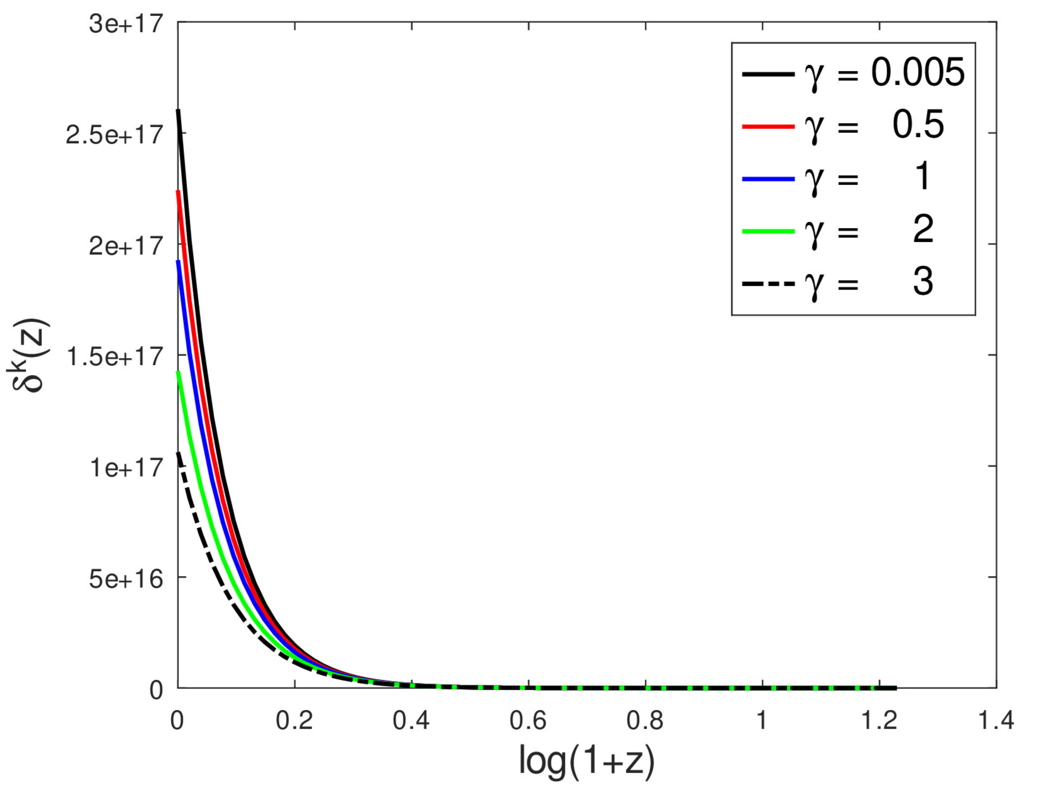
• Increasing $\alpha$ decreases the late-time perturbation amplitude in the short-wavelength regime, but this effect is reversed for $z\gtrsim 0.65$;
• Increasing $\alpha$ increases the perturbation amplitude in the long-wavelength regime;
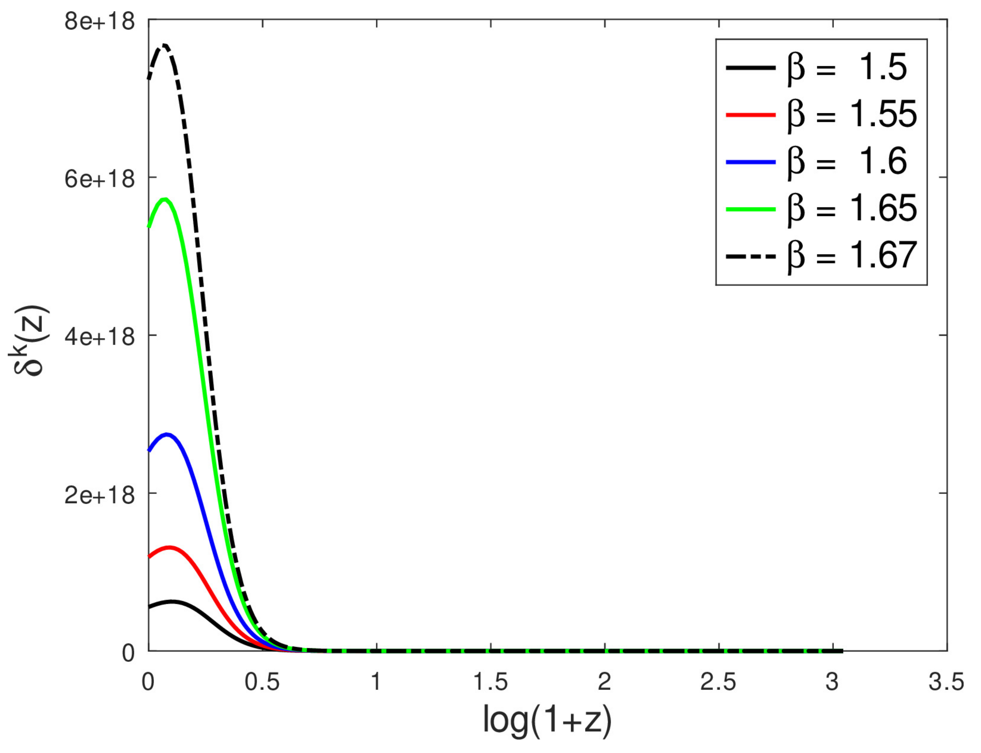
• Increasing $\beta$ increases the perturbation amplitudes in both the short- and long-wavelength regimes;
• Increasing n increases the perturbation amplitudes in both the short- and long-wavelength regimes.

5. Discussions and Conclusions

In this work, we have shown that introducing viscosity to the cosmic fluid not only affects the background expansion history, as shown in the results of Figure 1 and Figure 2, but also the rate at which structures grow. We have demonstrated this by first looking at the rate of structure growth in pure GR with and without the cosmological constant (and assuming a non-evolving gravitational constant G), depicted in Figure 4. As expected, the amplitudes’ comparison shows structure growth in $\Lambda$CDM is slower compared to pure GR, as structures have less time to coalesce and grow in an accelerated background. Next, we showed in Figure 5 that more structures can be expected in a Bianchi-V universe with evolving $\Lambda$ and G compared to both $\Lambda$CDM and pure GR cases. We then introduced the viscosity, and showed in Figure 6 and Figure 7 that structures grow even faster in this case, perhaps even suggesting nonlinear effects in the perturbations. Such divergences might be smoking-gun evidence of the failures of viscous Bianchi type-V models in the test of cosmological viability. Moreover, our results suggest that the longer the wavelength (i.e., the smaller the value of the wavenumber k and hence the dimensionless parameter $\gamma$), the larger the perturbation amplitudes, ceteris paribus. We have demonstrated this finding in Figure 8, Figure 9, Figure 10, Figure 11, Figure 12 and Figure 13, and it is in line with other findings [45,46,47,48] in the literature. In the short-wavelength regime, we noticed the perturbation amplitudes reaching maximum values at about the same redshift that the fractional background matter density peaked; see Figure 2, Figure 7, Figure 8, Figure 10 and Figure 12 for a comparison. Such a trend is not observed in the long-wavelength regime, and this may be because in the small-$\gamma$ limit, the wavelength-dependent contributions to the perturbations of Equation (52) are negligible compared to the other terms in the equation. However, this needs further scrutiny. As a follow-up exercise, it is worthwhile doing a cosmological viability test using more rigorous data analysis techniques involving simulated data values of the model compared against actual astronomical data.

References

- Perlmutter, S.; Gabi, S.; Goldhaber, G.; Goobar, A.; Groom, D.E.; Hook, I.M.; Pennypacker, C.R. Measurements of the Cosmological Parameters Ω and Λ from the First Seven Supernovae at z ≥ 0.35. Astrophys. J. 1997, 483, 565. [Google Scholar] [CrossRef]
- Perlmutter, S.; Aldering, G.; Della Valle, M.; Deustua, S.; Ellis, R.S.; Fabbro, S.; Kim, A.G. Discovery of a supernova explosion at half the age of the Universe. Nature 1998, 391, 51–54. [Google Scholar] [CrossRef]
- Perlmutter, S.; Aldering, G.; Goldhaber, G.; Knop, R.A.; Nugent, P.; Castro, P.G.; Hook, I.M. Measurements of Ω and Λ from 42 high-redshift supernovae. Astrophys. J. 1999, 517, 565. [Google Scholar] [CrossRef]
- Riess, A.G.; Filippenko, A.V.; Challis, P.; Clocchiatti, A.; Diercks, A.; Garnavich, P.M.; Leibundgut, B.R.U.N.O. Observational evidence from supernovae for an accelerating universe and a cosmological constant. Astron. J. 1998, 116, 1009. [Google Scholar] [CrossRef]
- Basilakos, S.; Sola, J. Growth index of matter perturbations in running vacuum models. Phys. Rev. D 2015, 92, 123501. [Google Scholar] [CrossRef]
- Gómez-Valent, A.; Karimkhani, E.; Solà, J. Background history and cosmic perturbations for a general system of self-conserved dynamical dark energy and matter. J. Cosmol. Astropart. Phys. 2015, 2015, 048. [Google Scholar] [CrossRef]
- Grande, J.; Sola, J.; Fabris, J.C.; Shapiro, I.L. Cosmic perturbations with running G and Λ. Class. Quantum Gravity 2010, 27, 105004. [Google Scholar] [CrossRef]
- Fabris, J.C.; Shapiro, I.L.; Sola, J. Density perturbations for a running cosmological constant. J. Cosmol. Astropart. Phys. 2007, 2007, 016. [Google Scholar] [CrossRef]
- Panotopoulos, G.; Rincón, Á. Growth of structures and redshift-space distortion data in scale-dependent gravity. Eur. Phys. J. Plus 2021, 136, 1–14. [Google Scholar] [CrossRef]
- Bonanno, A.; Saueressig, F. Asymptotically safe cosmology—A status report. Comptes Rendus Phys. 2017, 18, 254–264. [Google Scholar] [CrossRef]
- Bianchi, L. Memorie di Matematica e di Fisica della Societa Italiana delle Scienze, serie III. Tomo XI, 267 (1898); English translation. Gen. Rel. Grav. 2001, 33, 2157. [Google Scholar]
- Bianchi, L. Lezioni sulla Teoria dei Gruppi Continui finiti di Trasformazioni; Lectures on the Theory of Finite Continuous Transformation Groups; E. Spoerri: Pisa, Italy, 1918; see Sections 198–199, 550, (1902–1903). [Google Scholar]
- Dirac, P.A.M. The Cosmological Constants. Nature 1937, 139, 323. [Google Scholar] [CrossRef]
- Alfedeel, A.H.; Abebe, A.; Gubara, H.M. A Generalized Solution of Bianchi Type-V Models with Time-Dependent G and Λ. Universe 2018, 4, 83. [Google Scholar] [CrossRef]
- Alfedeel, A.H.; Abebe, A. Bianchi Type-V Solutions with Varying G and Λ: The General Case. Int. J. Geom. Methods Mod. Phys. 2020, 17, 2050076. [Google Scholar] [CrossRef]
- Vishwakarma, R.G. A model of the universe with decaying vacuum energy. Pramana J. Phys. 1996, 47, 41. [Google Scholar]
- Vishwakarma, R.G. Dissipative cosmology with decaying vacuum energy. Indian J. Phys. 1996, 70, 321. [Google Scholar]
- Vishwakarma, R.G. LRS Bianchi type-I models with a time-dependent cosmological constant. Phys. Rev. D 1999, 60, 3507. [Google Scholar] [CrossRef]
- Vishwakarma, R.G. A study of angular size-redshift relation for models in which Λ decays as the energy density. Class. Quantum Gravity 2000, 17, 3833. [Google Scholar] [CrossRef]
- Vishwakarma, R.G. Consequences on variable Λ-models from distant type Ia supernovae and compact radio sources. Class. Quantum Gravity 2001, 18, 11–59. [Google Scholar] [CrossRef]
- Vishwakarma, R.G. A model to explain varying Λ, G and σ2 simultaneously. Gen. Relativ. Gravit. 2005, 37, 1305. [Google Scholar] [CrossRef]
- Bali, R.; Singh, P.; Singh, J.P. Bianchi type-V viscous fluid cosmological models in presence of decaying vacuum energy. Astrophys. Space Sci. 2012, 341, 701–706. [Google Scholar] [CrossRef]
- Singh, J.P.; Baghel, P.S. Bulk viscous bianchi Type-V cosmological models with decaying cosmological term Λ. Int. Theor. Phys. 2010, 49, 2734–2744. [Google Scholar] [CrossRef]
- Padmanabhan, T.; Chitre, S.M. Viscous universes. Phys. Lett. A 1987, 120, 433–436. [Google Scholar] [CrossRef]
- Alfedeel, A.H.A.; Tiwari, R.K.; Sofuoğlu, D.; Abebe, A.; Hassan, E.I.; Shukla, B.K. A cosmological model with time dependent Λ, G and viscous fluid in General Relativity. Front. Astron. Space Sci. 2022, 9, 965652. [Google Scholar]
- Williams, J.G.; Turyshev, S.G.; Boggs, D.H. Lunar laser ranging tests of the equivalence principle with the earth and moon. Int. J. Mod. Phys. D 2009, 18, 1129–1175. [Google Scholar] [CrossRef]
- Copi, C.J.; Davis, A.N.; Krauss, L.M. New nucleosynthesis constraint on the variation of G. Phys. Rev. Lett. 2004, 92, 171301. [Google Scholar] [CrossRef]
- Pavon, D.; Bafaluy, J.; Jou, D. Causal Friedmann-Robertson-Walker cosmology. Class. Quantum Gravity 1991, 8, 347. [Google Scholar] [CrossRef]
- Maartens, R. Dissipative cosmology. Class. Quantum Gravity 1995, 12, 1455. [Google Scholar] [CrossRef]
- Zimdahl, W. Bulk viscous cosmology. Phys. Rev. D 1996, 53, 5483. [Google Scholar] [CrossRef]
- Santos, N.O.; Dias, R.S.; Banerjee, A. Isotropic homogeneous universe with viscous fluid. J. Math. Phys. 1985, 26, 878–881. [Google Scholar] [CrossRef]
- Gidelew, A.A. Covariant Perturbations in f(R)-Gravity of Multi-Component Fluid Cosmologies. Master’s Thesis, University of Cape Town, Cape Town, South Africa, 2009. [Google Scholar]
- Lifshitz, E.M. On the gravitational stability of the expanding universe. J. Phys. 1946, 10, 116–129. [Google Scholar]
- Bardeen, J.M. Gauge-invariant cosmological perturbations. Phys. Rev. D 1980, 22, 1882. [Google Scholar] [CrossRef]
- Kodama, H.; Sasaki, M. Cosmological perturbation theory. Prog. Theor. Phys. Suppl. 1984, 78, 1–166. [Google Scholar] [CrossRef]
- Ehlers, J. Beiträge zur relativistischen Mechanik kontinuierlicher Medien. In Abhandlungen der Mathematisch-Naturwissenschaftlichen Klasse; Akademie der Wissenschaften und der Literatur: Mainz, Germany, 1961; pp. 793–836. [Google Scholar]
- Hawking, S.W. Perturbations of an expanding universe. Astrophys. J. 1966, 145, 544. [Google Scholar] [CrossRef]
- Olson, D.W. Density perturbations in cosmological models. Phys. Rev. D 1976, 14, 327. [Google Scholar] [CrossRef]
- Ellis, G.F.; Bruni, M. Covariant and gauge-invariant approach to cosmological density fluctuations. Phys. Rev. D 1989, 40, 1804. [Google Scholar] [CrossRef]
- Dunsby, P.K.; Bruni, M.; Ellis, G.F. Covariant perturbations in a multifluid cosmological medium. Astrophys. J. 1992, 395, 54–74. [Google Scholar] [CrossRef]
- Bruni, M.; Dunsby, P.; Ellis, G.F.R. Cosmological perturbations and the physical meaning of gauge-invariant variables. Astrophys. J. 1992, 395, 34. [Google Scholar] [CrossRef]
- Clarkson, C.A.; Barrett, R.K. Covariant perturbations of Schwarzschild black holes. Class. Quantum Gravity 2003, 20, 3855. [Google Scholar] [CrossRef]
- Carloni, S.; Dunsby, P.K.S.; Troisi, A. Evolution of density perturbations in f(R) gravity. Phys. Rev. D 2008, 77, 024024. [Google Scholar] [CrossRef]
- Abebe, A.; Abdelwahab, M.; De la Cruz-Dombriz, Á.; Dunsby, P.K. Covariant gauge-invariant perturbations in multifluid f(R) gravity. Class. Quantum Gravity 2012, 29, 135011. [Google Scholar] [CrossRef]
- Sami, H.; Sahlu, S.; Abebe, A.; Dunsby, P.K. Covariant density and velocity perturbations of the quasi-Newtonian cosmological model in f(T) gravity. Eur. Phys. J. C 2021, 81, 1–17. [Google Scholar] [CrossRef]
- Sahlu, S.; Ntahompagaze, J.; Abebe, A.; de la Cruz-Dombriz, A.; Mota, D.F. Scalar perturbations in f(T) gravity using the 1 + 3 covariant approach. Eur. Phys. J. C 2020, 80, 1–19. [Google Scholar] [CrossRef]
- Hough, R.; Sahlu, S.; Sami, H.; Elmardi, M.; Swart, A.M.; Abebe, A. Confronting the Chaplygin gas with data: Background and perturbed cosmic dynamics. arXiv 2021, arXiv:2112.11695. [Google Scholar]
- Sami, H.; Abebe, A. Perturbations of quasi-Newtonian universes in scalar–tensor gravity. Int. J. Geom. Methods Mod. Phys. 2021, 18, 2150158. [Google Scholar] [CrossRef]
- Aghanim, N.; Akrami, Y.; Ashdown, M.; Aumont, J.; Baccigalupi, C.; Ballardini, M.; Roudier, G. Planck 2018 results-VI. Cosmological parameters. Astron. Astrophys. 2020, 641, A6. [Google Scholar]
Disclaimer/Publisher’s Note: The statements, opinions and data contained in all publications are solely those of the individual author(s) and contributor(s) and not of MDPI and/or the editor(s). MDPI and/or the editor(s) disclaim responsibility for any injury to people or property resulting from any ideas, methods, instructions or products referred to in the content. |
© 2023 by the authors. Licensee MDPI, Basel, Switzerland. This article is an open access article distributed under the terms and conditions of the Creative Commons Attribution (CC BY) license (https://creativecommons.org/licenses/by/4.0/).
Share and Cite
Abebe, A.; Alfedeel, A.H.A.; Sofuoğlu, D.; Hassan, E.I.; Tiwari, R.K. Perturbations in Bianchi-V Spacetimes with Varying Λ, G and Viscous Fluids. Universe 2023, 9, 61. https://doi.org/10.3390/universe9020061
Abebe A, Alfedeel AHA, Sofuoğlu D, Hassan EI, Tiwari RK. Perturbations in Bianchi-V Spacetimes with Varying Λ, G and Viscous Fluids. Universe. 2023; 9(2):61. https://doi.org/10.3390/universe9020061
Chicago/Turabian StyleAbebe, Amare, Alnadhief H. A. Alfedeel, Değer Sofuoğlu, Eltegani I. Hassan, and Rishi Kumar Tiwari. 2023. "Perturbations in Bianchi-V Spacetimes with Varying Λ, G and Viscous Fluids" Universe 9, no. 2: 61. https://doi.org/10.3390/universe9020061
APA StyleAbebe, A., Alfedeel, A. H. A., Sofuoğlu, D., Hassan, E. I., & Tiwari, R. K. (2023). Perturbations in Bianchi-V Spacetimes with Varying Λ, G and Viscous Fluids. Universe, 9(2), 61. https://doi.org/10.3390/universe9020061