Abstract
In the extended scalar sector of the SMASH (Standard Model - Axion-Seesaw-Higgs portal inflation) framework, we conduct a phenomenological investigation of the observable effects. In a suitable region of the SMASH scalar parameter spaces, we solve the vacuum metastability problem and discuss the one-loop correction to the triple Higgs coupling, . The and SM Higgs quartic coupling corrections are found to be proportional to the threshold correction. A large correction (≳5%) implies vacuum instability in the model and thus limits the general class of theories that use threshold correction. We performed a full two-loop renormalization group analysis of the SMASH model. The SMASH framework has also been used to estimate the evolution of lepton asymmetry in the universe.
Keywords:
Higgs portal inflation; beyond the standard model; SMASH; Higgs triple coupling; Higgs trilinear coupling PACS:
12.60.-i; 14.80.Cp; 12.10.Kt; 11.10.Hi
1. Introduction
After the discovery of the Standard Model (SM) Higgs boson [1,2], every elementary particle of the SM has been confirmed to exist. Even though the past forty years have been a spectacular triumph for the SM, the mass of the Higgs boson ( GeV) [3] poses a serious problem for the SM [4]. It is well-known that the SM Higgs potential is metastable [5], as the sign of the quartic coupling, , turns negative at instability scale GeV. On the other hand, the SM is devoid of non-perturbative problems since the non-perturbative scale , where GeV is the Planck scale, but still there are studies on non-perturbative effects of the SM [6,7,8,9,10]. In the post-Planckian regime, effects of quantum gravity are expected to dominate, and the non-perturbative scale is therefore well beyond the validity region of the SM, unlike the instability scale. The largest uncertainties in SM vacuum stability are driven by top quark pole mass and the mass of the SM Higgs boson [11]. The current data are in significant tension with the stability hypothesis, making it more likely that the universe is in a false vacuum state [12,13,14,15]. The expected lifetime of vacuum decay to a true vacuum is extraordinarily long, and it is unlikely to affect the evolution of the universe [16,17]. However, it is unclear why the vacuum state entered into a false vacuum to begin with during the early universe. In this post-SM era, the emergence of vacuum stability problems (among many others) forces the particle theorists to expand the SM in such a way that the will stay positive during the run all the way up to the Planck scale.
It is possible that at or below the instability scale, heavy degrees of freedom originating from a theory beyond the SM start to alter the running of the SM parameters of renormalization group equations (RGE). It has been shown that incorporating the Type-I seesaw mechanism [18,19,20,21,22,23,24,25,26,27,28] will have a large destabilizing effect if the neutrino Yukawa couplings are large [29], and an insignificantly small effect if they are small. Thus, to solve the vacuum stability problem simultaneously with neutrino mass, a larger theory extension is required. Embedding the invisible axion model [30,31,32] together with the Type-I seesaw was considered in [33,34]. The axion appears as a phase of a complex singlet scalar field. This approach aims to solve the vacuum stability problem by proving that the universe is currently in a true vacuum. The scalar sector of such a theory may stabilize the vacuum with a threshold mechanism [35,36]. The effective SM Higgs coupling gains a positive correction at , where is the Higgs doublet-singlet portal coupling and is the quartic coupling of the new scalar.
Corrections altering in such a model would also induce corrections to the triple Higgs coupling, , where GeV is the SM Higgs vacuum expectation value (VEV) [37,38,39]. The triple Higgs coupling is uniquely determined by the SM but is unmeasured. In fact, the Run 2 data from the Large Hadron Collider (LHC) has only been able to determine the upper limit of the coupling to be 12 times the SM prediction [3]. Therefore, future prospects of measuring a deviation of triple Higgs coupling by the high-luminosity upgrade of the LHC (HL-LHC) [40,41] or by a planned next-generation Future Circular Collider (FCC) [42,43,44,45,46,47,48,49] give us hints of the structure of the scalar sector of a beyond-the-SM theory. Previous work has shown that large corrections to triple Higgs coupling might originate from a theory with one extra Dirac neutrino [50,51], inverse seesaw model [52], two Higgs doublet model [38,39,53,54], one extra scalar singlet [37,55,56] or in the Type II seesaw model [57].
The complex singlet scalar, and consequently, the corresponding threshold mechanism, is embedded in a recent SMASH [58,59,60] theory, which utilizes it at and . The mechanism turns out to be dominant unless the new Yukawa couplings of SMASH are . In addition to its simple scalar sector extension, SMASH includes electroweak singlet quarks Q and and three heavy right-handed Majorana neutrinos , and to generate masses for neutrinos.
The structure of this paper is as follows: In Section 2, we summarize the SMASH model and cover the relevant details of its scalar sector. We also establish the connection between the threshold correction and the leading order correction. In Section 3, we discuss the methods, numerical details, RGE running, and our choice of benchmark points. Our results are presented in Section 4, where the viable parameter space is constrained by various current experimental limits. In SMASH, one can obtain at most ∼5% correction to while simultaneously stabilizing the vacuum. We give our short conclusions on Section 5.
2. Theory
The SMASH framework [58,59,60] expands the scalar sector of the SM by introducing a complex singlet field
where and A (the axion) are real scalar fields, and is the VEV of the complex singlet. The scalar potential of SMASH is then
Defining and , in basis (), the scalar mass matrix of this potential is
which has eigenvalues
and
At the heavy singlet limit
and
Defining threshold correction in Equation (13),
and
The first term in the Equation (9) is the leading component.
The SMASH framework also includes a new quark-like field, Q, which has color but is an electro-weak singlet. It gains its mass via the Higgs mechanism, through a complex singlet . It arises from the Yukawa term
We will show later that is forbidden by the vacuum stability requirement. The hypercharge of Q is chosen to be , even though is possible. Our analysis is almost independent of the hypercharge assignment.
Threshold correction: Consider an energy scale below , where the heavy scalar is integrated out. The low-energy Higgs potential should match the SM Higgs potential
It turns out that the quartic coupling we measure has an additional term
Since the SM Higgs quartic coupling will be approximately , the threshold correction
should have a minimum value close to or slightly larger to push the high-energy counterpart to positive value all the way up to . A too-large correction will, however, increase too rapidly, exceeding the perturbativity limit . We demonstrate the conditions for in Section 4. Similar to , the SM Higgs quadratic parameter gains a threshold correction
In the literature [35,36], there are two possible ways of implementing this threshold mechanism. One may start by solving the SM RGE’s up to , where the new singlet effects kick in, and the quadratic and quartic couplings gain sudden increments. Continuation of RGE analysis to even higher scales then requires utilizing the new RGE’s up to the Planck scale.
Another approach is to only solve the new RGEs on the SM scale while ignoring the low-scale SM RGEs entirely. We will use the former approach.
One-loop correction to triple Higgs coupling: The portal term of the Higgs potential contains the trilinear couplings for and vertices. The vertex factors for and vertices are introduced in Figure 1. The one-loop diagrams contributing to SM triple Higgs coupling are in Figure 2. We denote the SM tree-level triple Higgs coupling as . The correction is gained by adding all the triangle diagrams (taking into account the symmetry factors)
Here, p and q are the external momenta and the loop integral is defined as
The contribution from diagram Figure 3 is subleading, since it is proportional to .
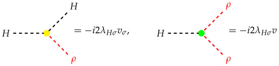
Figure 1.
Vertex factors on trilinear vertices involving the SM Higgs boson as well as a real singlet . They can be derived from Equation (2). We denote and its propagator by red color.
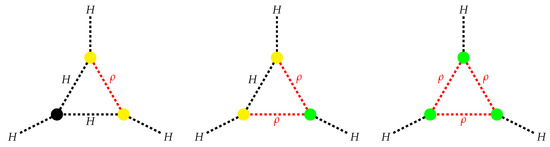
Figure 2.
One-loop corrections to SM triple Higgs coupling induced by the existence of an extra scalar singlet. In Equation (15), the correction is derived.
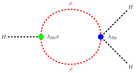
Figure 3.
One-loop SM triple Higgs coupling correction diagram with a cubic vertex and a quartic vertex.
The process is disallowed for on-shell external momenta, so at least one of them must be off-shell. Specifically, the momentum-dependent correction to the triple coupling at the tree-level is an effective coupling that enters the specific process with one off-shell Higgs decaying into two real Higgses. Note that the correction is dependent on the Higgs off-shell momentum , which we assume to be at TeV at the LHC and HL-LHC. The first diagram is dominant due to the heaviness of the scalar. Therefore, we may ignore the subleading contributions of diagrams involving two or more propagators. We integrate out the heavy scalar, causing the finite integral in Equation (16) to be logarithmically divergent. We calculate the finite part of it using dimensional regularization and obtain
where and is the regularization scale1. We have used the modified minimal subtraction scheme (), where the terms and Euler–Mascheroni constant emerging in the calculation are absorbed to the regularization scale . For calculations, we use the value TeV. It is especially interesting to see that at the leading order, the triple Higgs coupling correction is proportional to the threshold corrections. This intimate connection forbids a too-large correction. In fact, the bound from vacuum stability turns out to constrain the triple Higgs coupling correction to ≲, as we shall see in Section 4. Consequently, if LHC or HL-LHC manages to measure a correction to , this will rule out theories that utilize exclusively threshold correction mechanisms as a viable solution to the vacuum stability problem. Indeed, there are alternate ways to produce large without expanding the scalar sector [50,52].
It should be noted that loop corrections contributing to the final to-be-observed value are included in the SM. Indeed, experiments are measuring , where the SM one-loop correction depends on the Higgs off-shell momentum. At the TeV scale we are considering, the SM 1-loop correction amounts to approximately [50].
Light neutrino masses: The neutrino sector of SMASH is able to generate correct neutrino masses and observe the baryon asymmetry of the universe with suitable benchmarks. The relevant Yukawa terms for neutrinos in the model are
We take a simplified approach: Dirac and Majorana Yukawa matrices ( and , respectively) are assumed to be diagonal.
To generate baryonic asymmetry in the universe, SMASH utilizes the thermal leptogenesis scenario [61], which generates lepton asymmetry in the early universe and leads to baryon asymmetry. In the scenario, heavy neutrinos require a sufficient mass hierarchy [62,63] and one or more Yukawa couplings must have complex CP phase factors. We assume the CP phases are radians to near-maximize the CP asymmetry [64,65,66]
If the CP violation is maximal, the largest value is obtained. To produce matter–antimatter asymmetry in the universe, a large asymmetry is required. Following [58], we set the heavy neutrino mass hierarchy at , corresponding to . These choices give the full neutrino mass matrix
which is in block form, and contains two free parameters: and . Here, is the Dirac mass term and is the Majorana mass term. Light neutrino masses are then generated via the well-known Type I seesaw mechanism [18,19,20,21,22,23,24,25,26,27,28], by block diagonalizing the full neutrino mass matrix .
It is possible to obtain light neutrino masses consistent with experimental constraints from atmospheric and solar mass splittings and [67] and cosmological constraint eV [68,69,70,71,72,73] (corresponding to (0.055) eV with normal (inverse) neutrino mass ordering, from Equations (10)–(12) and Figure 1 of [74] for upper bound), assuming the standard CDM cosmological model [74,75,76,77,78]. However, the total mass should not be less than 0.06 (0.10) eV for normal (inverse) hierarchy as per Equation (13) of [74].
The light neutrino mass matrix is
After removing the irrelevant sign via field redefinition,
where we have denoted and assumed normal mass ordering . This gives the neutrino masses . We do not know the absolute masses, but the mass squared differences have been measured by various neutrino oscillation experiments [67,79]. Nevertheless, their values provide two constraints, leaving three free parameters. However, the heavy neutrino Yukawa couplings must be no larger than to avoid vacuum instability [59].
In addition, an order-of-magnitude estimate of the generated matter–antimatter asymmetry (baryon-to-photon ratio) is directly proportional to the CP asymmetry
where 0.01–0.1 is an efficiency factor. We arrive at
which, in principle, can be consistent with the observed . To achieve successful resonance leptogenesis, should be between and GeV (Table 1). We will provide suitable benchmark points in the next section. The estimation of lepton asymmetry, which is one of the crucial implications of SMASH as the framework claims to solve the matter-asymmetry issue since the scenario only consists of the decay and inverse decay of or to . The leptogenesis evolution for the benchmark values shown in Table 2 is in Figure 4.

Table 1.
Used benchmark points (BP) in our analysis. Note that we assume specific texture to right-handed neutrino Yukawa matrix .
Table 2.
The computed values of neutrino masses for normal hierarchy (), the sum of light neutrino masses, and light neutrino mass squared differences. These neutrino masses are within experimental limits [67,68,69,70,71,72,73,79]. meV is Milli() (symbol m) eV.
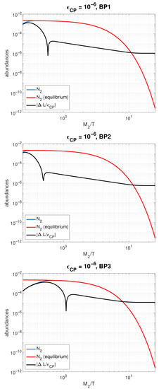
Figure 4.
The evolution of the “abundance” of in blue, the “abundance” of in thermal equilibrium in red, and the lepton asymmetry generated by the CP violating decays and inverse decays of divided by the CP asymmetry parameter in black. T is the temperature of the universe in GeV, as well as the mass of heavy neutrinos in GeV. is the number of changes in lepton number over entropy density s.
We will investigate the influence of , , and oscillations (i.e., right-handed neutrino oscillations) on leptogenesis evolutions, predict baryon-to-photon ratios for different set masses of light active left-handed neutrinos, and evaluate a more precise value of by solving complicated Boltzmann equations in the future course of analysis in the SMASH framework.
3. Methods
We generate the suitable benchmark points demonstrating different physics aspects of the model in the neutrino sector by fitting in the known neutrino mass squared differences , assuming normal mass ordering . This leaves three free neutrino parameters, the values of which we generate by logarithmically distributed random sampling. These are the candidates for benchmark points. We then require that the candidate points be consistent with the bounds for the sum of light neutrino masses [68,69,70,71,72,73,74,75,76,77,78]. The next step is to choose suitable values for other unknown parameters, using the stability of the vacuum as a requirement.
The authors of [58] have generated the corrections to the two-loop functions of SMASH. We solve numerically the full two-loop 14 coupled renormalization group differential equations with SMASH corrections with respect to Yukawa (), gauge () and scalar couplings (), ignoring the light SM degrees of freedom, from to Planck scale. We assume Yukawa matrices are on a diagonal basis, with the exception of . We use the scheme for the running of the RGE’s. Since the top quark mass is different from its pole mass, the difference is taken into account via the relation [80]
where at . We define the Higgs quadratic coupling as and quartic coupling as .
We use MATLAB R2019’s ode45-solver. See Table 1 for the used SMASH benchmark points and Table 3 for our SM input [3]. Our scale convention is GeV.
Table 3.
Used SM inputs in our analysis, at GeV, with the exception of top mass, which is evaluated at . Masses and vacuum expectation values are in GeV units [3].
In some papers, the running of SM parameters () obeys the SM RGE’s without corrections from a more effective theory until some intermediate scale [35], after which the SM parameters gain threshold correction (where it is relevant) and the running of all SM parameters follows the new RGE’s from that point onwards. We choose to utilize this approach while acknowledging an alternative approach, where the threshold correction is applied at the beginning () [36], and both approaches give almost the same results. As previously stated, SM Higgs quadratic and quartic couplings will gain the threshold correction.
Our aim is to find suitable benchmark points, which:
- Allow the quartic and Yukawa couplings of the theory to remain positive and perturbative up to the Planck scale;
- Utilize a threshold correction mechanism to via ;
- Avoid the overproduction of dark radiation via the cosmic axion background (requiring );
- Produce a significant contribution matter–antimatter asymmetry via leptogenesis (requiring hierarchy between the heavy neutrinos);
- Produce a ∼5% correction to triple Higgs coupling .
4. Results
Stability of vacuum: We have plotted how the running of the SM quartic coupling, changes with each benchmark point in Figure 5. Note that all the threshold corrections are utilized well before the SM instability scale . One can choose if is ensured. This is the case with BP3.
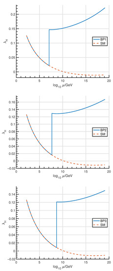
Figure 5.
Running of SM Higgs quartic coupling in Standard Model (dashed line) and in SMASH with benchmark points BP1–BP3 (solid line). Threshold correction is utilized at .
We numerically scanned over the parameter space GeV and GeV to analyze vacuum stability in three different benchmark points BP1–BP3. Our results for the chosen benchmarks are in Figure 6, where the SM best fit is denoted by a red star. Clearly, the electroweak vacuum is stable with our benchmark points, and it is assigned to GeV and GeV [3]. For every case, we investigated the running of the quartic couplings of the scalar potential. We used the following stability conditions
and for [35]
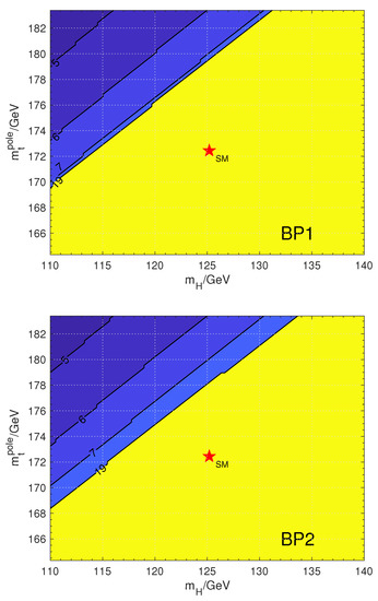
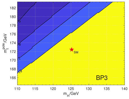
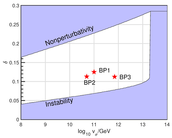
Figure 6.
Vacuum stability of SMASH in plane with benchmark points BP1–BP3. The red star corresponds to the SM best-fit value. The height and width of the star correspond to the present uncertainties. The vacuum is stable in the yellow region. The contour numbers n correspond to the vacuum instability scale GeV.
If one or more conditions are not met on the scale , we denote this point as unstable. If any of the quartic couplings rises above , we denote this point non-perturbative.
We chose the new scalar parameters in such a way that the threshold correction is large but allowed, . This changes the behavior of the coupling’s running so that after the correction, the increases in energy instead of decreasing, the opposite of the coupling’s running in a pure SM scenario. A too-large threshold correction will have an undesired effect, lowering the non-perturbative scale to energies lower than the Planck scale. These effects are visualized in Figure 7, where for each benchmark point kept at its designated value in Table 1. Instead, we let the portal coupling, , vary between 0 and . This demonstrates the small range of viable parameters space.
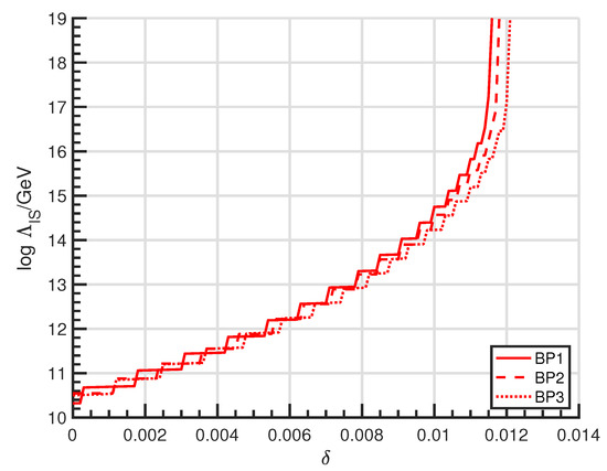
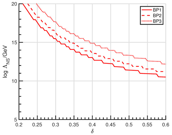
Figure 7.
The rise of the instability scale (above) and the fall of the non-perturbative scale (below) as a function of threshold correction , for BP1–BP3.
We have also investigated the significance of on the bounds of threshold correction . A choice of is available as long as GeV. This can be seen clearly from Figure 8. Given a fixed , the result is independent of and . The lower and higher bound for increases as a function of . Instability bound increases, since the needed vacuum-stabilizing threshold effect increases as one approaches the SM instability scale . At GeV, the , so the quartic coupling will turn negative before threshold correction is utilized. On the other hand, the non-perturbative scale increases, since, as the cutoff point increases, the quartic coupling decreases and correspondingly, the largest possible threshold correction increases.
Our next scan was over the new quartic couplings, and . The scalar potential is stable and the couplings remain perturbative at only a narrow band, where 0.01–0.1, see Figure 9. If one considers small , the SM Higgs quartic coupling will decrease to near zero at . This corresponds to a region near the left side of the stability band. In contrast, we chose our benchmarks with large , placing it near the right side of the stability band, corresponding to the large value of at . This was a deliberate choice to maximize the correction to .
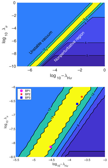
Figure 9.
(Above): Different regions in the logarithmic plane. The contour numbers n above the yellow band correspond to the vacuum instability scale GeV. Below the yellow band, the contour numbers m correspond to the non-perturbative scale GeV. The color coding is interpreted as in Figure 6. For non-perturbative scale calculations, we used BP1. (Below): Zoomed-in detail of the figure above, showing in addition our chosen benchmarks.
In addition, we have scanned the Dirac neutrino and new quark-like particle Yukawa couplings ( and , respectively) over and , keeping and small, real2 and positive but non-zero. See Figure 10 for details corresponding to each benchmark point. There, we point to an area producing a stable vacuum. The Dirac neutrino Yukawa couplings may have a maximum value of , but a more stringent constraint is found for . It should be noted that even though, from the vacuum instability point of view, , this does not imply , since both are in principle free parameters. See Table 2 for computed values for neutrino masses for normal hierarchy () corresponding to each benchmark. Note that all BP1–BP3 produce a value of baryon-to-photon ratio comparable to experimental values and a mass of axion consistent with axion dark matter scenario, because it requires axion decay constant to be GeV [30,31,32].
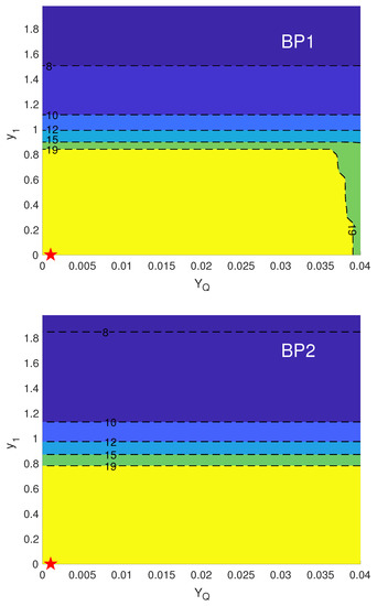
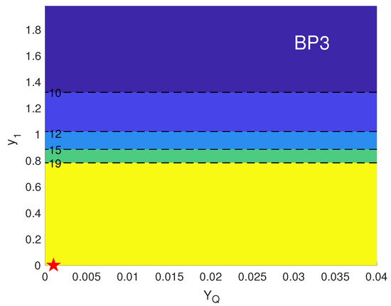
Figure 10.
Vacuum instability scales in plane in benchmark points BP1–BP3. The red star corresponds to the chosen benchmark point value. The color coding and the contour numbers are interpreted as in Figure 6.
In Figure 4, we show the evolution of or abundance, as well as the lepton asymmetry generated by the CP violating decays and inverse decays of or , divided by the CP asymmetry parameter as per [62]. The resulting lepton asymmetry is translated to baryon asymmetry via the sphaleron process with a fraction. We have also shown the or abundance in thermal equilibrium. The number density n of particles decreases in an expanding universe if there are now particle number-changing interactions. However, the ratio of number density n to entropy density s, that is, “abundance” , is constant. Changing “abundance” during the early universe thus indicates particle interactions, or in our case, or decays and inverse decays. A corresponding mass hierarchy for right-handed neutrinos implies an upper bound of to [63,81].
Correction to SM triple Higgs coupling: According to PDG [3], the largest possible experimental value for is 12 times the SM prediction3, from Run 2 data for the channel alone. The real singlet scalar mixes with the SM Higgs, providing a one-loop correction to SM triple Higgs coupling . We scanned the parameter space with and . At each point, we calculated the correction to . See Figure 11 for details. We identified a section of parameter space excluded by triple Higgs coupling searches from LHC run 2 and determined the area sensitive to future experiments, namely, HL-LHC and FCC-hh. We assume HL-LHC uses 14 TeV center-of-mass energy and integrated luminosity , for FCC-hh we assume center-of-mass energy 100 TeV and integrated luminosity . The relative correction in Table 4 is calculated with respect to the SM tree-level prediction. We chose our benchmark points in a way that their correction to triple Higgs coupling will be borderline observable at FCC-hh [82], that is, the correction will be ∼5%. Thus, in BP3 for a factor of 10 larger is necessary for stable vacuum and FCC-hh better detection shown in Figure 11. Future FCC-hh accelerator is sensitive to ∼5% deviation of the Standard Model prediction. This is demonstrated by the benchmark points we have chosen. Although the model’s stable region allows for even smaller deviations, part of the region is still accessible by FCC-hh.
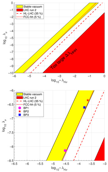
Figure 11.
(Above): Different regions in the logarithmic plane. The yellow band corresponds to a stable vacuum configuration. The red area is excluded from the second run of the Large Hadron Collider since the triple Higgs coupling corrections to SMASH would be too large. The dashed line corresponds to the expected sensitivity of the high-luminosity LHC, and the dotted line to the expected sensitivity of the Future Circular Collider in hadronic collision mode. (Below): Zoomed-in detail of the figure above, showing in addition our chosen benchmarks.
Table 4.
The computed values of threshold correction , BSM scalar masses and , baryon-to-photon ratio , quartic self-couplings at , correction to the triple Higgs coupling compared to the SM prediction.
This has implications for a general class of BSM theories that utilize complex singlet scalars and other new non-scalar fields. If the corrections from non-scalar contributions to SM triple Higgs and quartic couplings are tiny, any large correction to (such as a discrepancy from a SM value measured by the HL-LHC) would rule out such a class of theories, including SMASH. It will be up to the HL-LHC experiment to determine whether this is the case.
5. Conclusions
We have investigated suitable benchmark scenarios for the simplest SMASH model regarding the scalars and neutrinos, constraining the new Yukawa couplings and scalar couplings via the vacuum stability and theory perturbativity requirements. The model can easily account for the neutrino sector, predicting the correct light neutrino mass spectrum while evading the experimental bounds for right-handed heavy sterile Majorana neutrinos. In [58], the authors of the SMASH model performed a one-loop RGE analysis of the model and presented the two-loop RGE’s. We have extended the analysis to two-loop to gain the increased precision needed for the combined achievement of a stabilized electroweak vacuum and a large-enough triple Higgs coupling correction to be sensitive at FCC-hh. To the best of the authors’ knowledge, this is the first report on the connection between threshold correction to and one-loop correction to .
We found an interesting interplay between the triple Higgs coupling correction and the SM Higgs quartic coupling correction. A successful vacuum stabilization mechanism (threshold mechanism) in SMASH is consistent with small triple Higgs coupling corrections, requiring it to be at most ∼. Since the is proportional to the threshold correction , a large correction to inevitably leads to a large threshold correction. Detecting a correction larger than ∼ is within the sensitivity of a future high-luminosity upgrade of the LHC [40,41]. If detected, it would, therefore, rule out the simplest scalar sector of the model completely. This would force the model to develop non-minimal alternatives, such as an additional scalar doublet or triplet instead of a singlet. These alternatives were considered by the authors of the SMASH model in their recently updated study [60]. The lepton asymmetry is around to for the present-day scenario of the universe, which can be verified experimentally [83] at the FCC [47], LHC [84], and by the Circular Electron Positron Collider (CEPC) [85] for the SMASH framework.
Author Contributions
Conceptualization, C.R.D. and K.H.; methodology, T.J.K.; software, T.J.K.; validation, C.R.D. and T.J.K.; formal analysis, C.R.D. and K.H.; investigation, C.R.D.; resources, T.J.K.; data curation, T.J.K.; writing—original draft preparation, T.J.K.; writing—review and editing, C.R.D.; visualization, C.R.D.; supervision, K.H. All authors have read and agreed to the published version of the manuscript.
Funding
This research received no external funding.
Data Availability Statement
Data is unavailable due to privacy.
Acknowledgments
CRD expresses gratitude to Professor D.I. Kazakov (Director, BLTP, JINR) for support and is also thankful to Alexander Bednyakov (BLTP, JINR) for the insightful discussions.
Conflicts of Interest
The authors declare no conflict of interest.
Notes
| 1 | We integrate out at the tree level and then compute loop corrections to the triple Higgs coupling in the resulting effective theory with integrated out. By construction, the effective theory is just the SM plus higher-dimensional operators suppressed by inverse powers of . Deviations from the SM triple Higgs coupling can then only come from the effects of the higher-dimensional operators, and so these deviations should involve the inverse powers of which are in Equation (17). In other words, in the limit , one should recover the SM result, which Equation (17) does satisfy. |
| 2 | We acknowledge that neutrino Yukawa coupling matrix should be complex in order to allow the leptogenesis scenario to work. The vacuum stability analysis, however, is unaffected by this, and we can safely ignore the imaginary parts of the Yukawa couplings in this part of the analysis. |
| 3 | https://pdg.lbl.gov/2022/reviews/rpp2022-rev-higgs-boson.pdf, page 29–30, chapter 11, Section 3.4.2 and page 66, chapter 11, Section 6.2.5. |
References
- Aad, G.; Abajyan, T.; Abbott, B.; Abdallah, J.; Khalek, S.A.; Abdelalim, A.A.; Aben, R.; Abi, B.; Abolins, M.; AbouZeid, O.S.; et al. Observation of a new particle in the search for the Standard Model Higgs boson with the ATLAS detector at the LHC. Phys. Lett. B 2012, 716, 1–29. [Google Scholar] [CrossRef]
- Chatrchyan, S.; Khachatryan, V.; Sirunyan, A.M.; Tumasyan, A.; Adam, W.; Aguilo, E.; Bergauer, T.; Dragicevic, M.; Erö, J.; Fabjan, C.; et al. Observation of a New Boson at a Mass of 125 GeV with the CMS Experiment at the LHC. Phys. Lett. B 2012, 716, 30–61. [Google Scholar] [CrossRef]
- Workman, R.L.; Burkert, V.D.; Crede, V.; Klempt, E.; Thoma, U.; Tiator, L.; Agashe, K.; Aielli, G.; Allanach, B.C.; Amsler, C.; et al. Review of Particle Physics. PTEP 2022, 2022, 083C01. [Google Scholar] [CrossRef]
- Bass, S.D.; De Roeck, A.; Kado, M. The Higgs boson implications and prospects for future discoveries. Nat. Rev. Phys. 2021, 3, 608–624. [Google Scholar] [CrossRef]
- Alekhin, S.; Djouadi, A.; Moch, S. The top quark and Higgs boson masses and the stability of the electroweak vacuum. Phys. Lett. B 2012, 716, 214–219. [Google Scholar] [CrossRef]
- Nielsen, H.B.; Froggatt, C.D. Anomalies from Non-Perturbative Standard Model Effects. arXiv 2019, arXiv:1905.00070. [Google Scholar]
- Arbuzov, B.A.; Zaitsev, I.V. Calculation of the contribution to muon g − 2 due to the effective anomalous three boson interaction and the new experimental result. Int. J. Mod. Phys. A 2021, 36, 2150223. [Google Scholar] [CrossRef]
- Arbuzov, B.A. The discrepancy in the muon g − 2 is a non-perturbative effect of the Standard Model. arXiv 2013, arXiv:1304.7090. [Google Scholar]
- Wang, J.; Wen, X.G. Nonperturbative definition of the standard models. Phys. Rev. Res. 2020, 2, 023356. [Google Scholar] [CrossRef]
- Arbuzov, B.A. Non-perturbative Effective Interactions in the Standard Model. In De Gruyter Studies in Mathematical Physics; De Gruyter: Berlin, Germany; Boston, MA, USA, 2014; Volume 23. [Google Scholar] [CrossRef]
- Bednyakov, A.V. An advanced precision analysis of the SM vacuum stability. Phys. Part. Nucl. 2017, 48, 698–703. [Google Scholar] [CrossRef]
- Abel, S.; Spannowsky, M. Observing the fate of the false vacuum with a quantum laboratory. PRX Quantum 2021, 2, 010349. [Google Scholar] [CrossRef]
- Markkanen, T.; Rajantie, A.; Stopyra, S. Cosmological Aspects of Higgs Vacuum Metastability. Front. Astron. Space Sci. 2018, 5, 40. [Google Scholar] [CrossRef]
- Lorenz, C.S.; Funcke, L.; Calabrese, E.; Hannestad, S. Time-varying neutrino mass from a supercooled phase transition: Current cosmological constraints and impact on the Ωm-σ8 plane. Phys. Rev. D 2019, 99, 023501. [Google Scholar] [CrossRef]
- Landim, R.G.; Abdalla, E. Metastable dark energy. Phys. Lett. B 2017, 764, 271–276. [Google Scholar] [CrossRef]
- Kohri, K.; Matsui, H. Electroweak Vacuum Instability and Renormalized Vacuum Field Fluctuations in Friedmann-Lemaitre-Robertson-Walker Background. Phys. Rev. D 2018, 98, 103521. [Google Scholar] [CrossRef]
- Masina, I. Higgs boson and top quark masses as tests of electroweak vacuum stability. Phys. Rev. D 2013, 87, 053001. [Google Scholar] [CrossRef]
- Fritzsch, H.; Gell-Mann, M.; Minkowski, P. Vecto—Like Weak Currents and New Elementary Fermions. Phys. Lett. B 1975, 59, 256–260. [Google Scholar] [CrossRef]
- Minkowski, P. μ→eγ at a Rate of One Out of 109 Muon Decays? Phys. Lett. B 1977, 67, 421–428. [Google Scholar] [CrossRef]
- Gell-Mann, M.; Ramond, P.; Slansky, R. Complex Spinors and Unified Theories. Conf. Proc. C 1979, 790927, 315–321. [Google Scholar]
- Yanagida, T. Horizontal Symmetry and Masses of Neutrinos. Prog. Theor. Phys. 1980, 64, 1103. [Google Scholar] [CrossRef]
- Mohapatra, R.N.; Senjanovic, G. Neutrino Mass and Spontaneous Parity Nonconservation. Phys. Rev. Lett. 1980, 44, 912. [Google Scholar] [CrossRef]
- Mohapatra, R.N.; Senjanovic, G. Neutrino Masses and Mixings in Gauge Models with Spontaneous Parity Violation. Phys. Rev. D 1981, 23, 165. [Google Scholar] [CrossRef]
- Schechter, J.; Valle, J.W.F. Neutrino Masses in SU(2) × U(1) Theories. Phys. Rev. D 1980, 22, 2227. [Google Scholar] [CrossRef]
- Magg, M.; Wetterich, C. Neutrino Mass Problem and Gauge Hierarchy. Phys. Lett. B 1980, 94, 61–64. [Google Scholar] [CrossRef]
- Glashow, S.L. The Future of Elementary Particle Physics. NATO Sci. Ser. B 1980, 61, 687. [Google Scholar] [CrossRef]
- Lazarides, G.; Shafi, Q. Neutrino Masses in SU(5). Phys. Lett. B 1981, 99, 113–116. [Google Scholar] [CrossRef]
- Gelmini, G.B.; Roncadelli, M. Left-Handed Neutrino Mass Scale and Spontaneously Broken Lepton Number. Phys. Lett. B 1981, 99, 411–415. [Google Scholar] [CrossRef]
- Bambhaniya, G.; Bhupal Dev, P.S.; Goswami, S.; Khan, S.; Rodejohann, W. Naturalness, Vacuum Stability and Leptogenesis in the Minimal Seesaw Model. Phys. Rev. D 2017, 95, 095016. [Google Scholar] [CrossRef]
- Abbott, L.F.; Sikivie, P. A Cosmological Bound on the Invisible Axion. Phys. Lett. B 1983, 120, 133–136. [Google Scholar] [CrossRef]
- Preskill, J.; Wise, M.B.; Wilczek, F. Cosmology of the Invisible Axion. Phys. Lett. B 1983, 120, 127–132. [Google Scholar] [CrossRef]
- Dine, M.; Fischler, W. The Not So Harmless Axion. Phys. Lett. B 1983, 120, 137–141. [Google Scholar] [CrossRef]
- Bertolini, S.; Di Luzio, L.; Kolešová, H.; Malinský, M. Massive neutrinos and invisible axion minimally connected. Phys. Rev. D 2015, 91, 055014. [Google Scholar] [CrossRef]
- Salvio, A. A Simple Motivated Completion of the Standard Model below the Planck Scale: Axions and Right-Handed Neutrinos. Phys. Lett. B 2015, 743, 428–434. [Google Scholar] [CrossRef]
- Elias-Miro, J.; Espinosa, J.R.; Giudice, G.F.; Lee, H.M.; Strumia, A. Stabilization of the Electroweak Vacuum by a Scalar Threshold Effect. J. High Energy Phys. 2012, 6, 031. [Google Scholar] [CrossRef]
- Lebedev, O. On Stability of the Electroweak Vacuum and the Higgs Portal. Eur. Phys. J. C 2012, 72, 2058. [Google Scholar] [CrossRef]
- He, S.P.; Zhu, S.H. One-loop radiative correction to the triple Higgs coupling in the Higgs singlet model. Phys. Lett. B 2017, 764, 31–37, Erratum in Phys. Lett. B 2019, 797, 134782. [Google Scholar] [CrossRef]
- Arhrib, A.; Benbrik, R.; El Falaki, J.; Jueid, A. Radiative corrections to the Triple Higgs Coupling in the Inert Higgs Doublet Model. J. High Energy Phys. 2015, 12, 007. [Google Scholar] [CrossRef]
- Arhrib, A.; Benbrik, R.; Chiang, C.W. Probing triple Higgs couplings of the Two Higgs Doublet Model at Linear Collider. Phys. Rev. D 2008, 77, 115013. [Google Scholar] [CrossRef]
- Cepeda, M.; Gori, S.; Ilten, P.; Kado, M.; Riva, F.; Abdul Khalek, R.; Aboubrahim, A.; Alimena, J.; Alioli, S.; Alves, A.; et al. Report from Working Group 2: Higgs Physics at the HL-LHC and HE-LHC. CERN Yellow Rep. Monogr. 2019, 7, 221–584. [Google Scholar] [CrossRef]
- Adhikary, A.; Banerjee, S.; Barman, R.K.; Bhattacherjee, B.; Niyogi, S. Higgs Self-Coupling at the HL-LHC and HE-LHC. Springer Proc. Phys. 2022, 277, 27–31. [Google Scholar] [CrossRef]
- Arkani-Hamed, N.; Han, T.; Mangano, M.; Wang, L.T. Physics opportunities of a 100 TeV proton–proton collider. Phys. Rept. 2016, 652, 1–49. [Google Scholar] [CrossRef]
- Baglio, J.; Djouadi, A.; Quevillon, J. Prospects for Higgs physics at energies up to 100 TeV. Rept. Prog. Phys. 2016, 79, 116201. [Google Scholar] [CrossRef] [PubMed]
- Contino, R.; Curtin, D.; Katz, A.; Mangano, M.L.; Panico, G.; Ramsey-Musolf, M.J.; Zanderighi, G.; Anastasiou, C.; Astill, W.; Bambhaniya, G.; et al. Physics at a 100 TeV pp collider: Higgs and EW symmetry breaking studies. arXiv 2016, arXiv:1606.09408. [Google Scholar]
- Myers, S. The Future Circular Collider: Its potential and lessons learnt from the LEP and LHC experiments. Res. Outreach 2022. [Google Scholar] [CrossRef]
- Benedikt, M.; Blondel, A.; Janot, P.; Mangano, M.; Zimmermann, F. Future Circular Colliders succeeding the LHC. Nat. Phys. 2020, 16, 402–407. [Google Scholar] [CrossRef]
- Blondel, A.; Janot, P. FCC-ee overview: New opportunities create new challenges. Eur. Phys. J. Plus 2022, 137, 92. [Google Scholar] [CrossRef]
- Myers, S. FCC: Building on the shoulders of giants. Eur. Phys. J. Plus 2021, 136, 1076. [Google Scholar] [CrossRef]
- Aleksa, M.; Allport, P.P.; Asai, S.; Ball, A.; Besana, M.I.; Bielert, E.R.; Bologna, S.; Boos, E.; Borgonovi, L.; Bosley, R.; et al. Conceptual design of an experiment at the FCC-hh, a future 100 TeV hadron collider. CERN Yellow Rep. Monogr. 2022, 2/2022, 1–304. [Google Scholar] [CrossRef]
- Baglio, J.; Weiland, C. Heavy neutrino impact on the triple Higgs coupling. Phys. Rev. D 2016, 94, 013002. [Google Scholar] [CrossRef]
- Baglio, J.; Weiland, C. Impact of heavy sterile neutrinos on the triple Higgs coupling. PoS 2017, EPS-HEP2017, 143. [Google Scholar] [CrossRef]
- Baglio, J.; Weiland, C. The triple Higgs coupling: A new probe of low-scale seesaw models. J. High Energy Phys. 2017, 4, 038. [Google Scholar] [CrossRef]
- Dubinin, M.N.; Semenov, A.V. Triple and quartic interactions of Higgs bosons in the general two Higgs doublet model. arXiv 1998, arXiv:hep-ph/9812246. [Google Scholar]
- Dubinin, M.N.; Semenov, A.V. Triple and quartic interactions of Higgs bosons in the two Higgs doublet model with CP violation. Eur. Phys. J. C 2003, 28, 223–236. [Google Scholar] [CrossRef]
- Kanemura, S.; Kikuchi, M.; Yagyu, K. Radiative corrections to the Higgs boson couplings in the model with an additional real singlet scalar field. Nucl. Phys. B 2016, 907, 286–322. [Google Scholar] [CrossRef]
- Kanemura, S.; Kikuchi, M.; Yagyu, K. One-loop corrections to the Higgs self-couplings in the singlet extension. Nucl. Phys. B 2017, 917, 154–177. [Google Scholar] [CrossRef]
- Aoki, M.; Kanemura, S.; Kikuchi, M.; Yagyu, K. Radiative corrections to the Higgs boson couplings in the triplet model. Phys. Rev. D 2013, 87, 015012. [Google Scholar] [CrossRef]
- Ballesteros, G.; Redondo, J.; Ringwald, A.; Tamarit, C. Standard Model—Axion—Seesaw—Higgs portal inflation. Five problems of particle physics and cosmology solved in one stroke. J. Cosmol. Astropart. Phys. 2017, 8, 001. [Google Scholar] [CrossRef]
- Ballesteros, G.; Redondo, J.; Ringwald, A.; Tamarit, C. Unifying inflation with the axion, dark matter, baryogenesis and the seesaw mechanism. Phys. Rev. Lett. 2017, 118, 071802. [Google Scholar] [CrossRef]
- Ballesteros, G.; Redondo, J.; Ringwald, A.; Tamarit, C. Several Problems in Particle Physics and Cosmology Solved in One SMASH. Front. Astron. Space Sci. 2019, 6, 55. [Google Scholar] [CrossRef]
- Fukugita, M.; Yanagida, T. Baryogenesis Without Grand Unification. Phys. Lett. B 1986, 174, 45–47. [Google Scholar] [CrossRef]
- Buchmuller, W.; Di Bari, P.; Plumacher, M. Cosmic microwave background, matter–antimatter asymmetry and neutrino masses. Nucl. Phys. B 2002, 643, 367–390, Erratum in Nucl. Phys. B 2008, 793, 362. [Google Scholar] [CrossRef]
- Davidson, S.; Ibarra, A. A Lower bound on the right-handed neutrino mass from leptogenesis. Phys. Lett. B 2002, 535, 25–32. [Google Scholar] [CrossRef]
- Buchmuller, W.; Di Bari, P.; Plumacher, M. Leptogenesis for pedestrians. Ann. Phys. 2005, 315, 305–351. [Google Scholar] [CrossRef]
- Buchmüller, W. Leptogenesis: Theory and Neutrino Masses. Nucl. Phys. B Proc. Suppl. 2013, 235–236, 329–335. [Google Scholar] [CrossRef]
- Buchmüller, W. Leptogenesis. Scholarpedia 2014, 9, 11471. [Google Scholar] [CrossRef]
- Esteban, I.; Gonzalez-Garcia, M.C.; Maltoni, M.; Schwetz, T.; Zhou, A. The fate of hints: Updated global analysis of three-flavor neutrino oscillations. J. High Energy Phys. 2020, 9, 178. [Google Scholar] [CrossRef]
- Aghanim, N.; Akrami, Y.; Ashdown, M.; Aumont, J.; Baccigalupi, C.; Ballardini, M.; Banday, A.J.; Barreiro, R.B.; Bartolo, N.; Basak, S.; et al. Planck 2018 results. VI. Cosmological parameters. Astron. Astrophys. 2020, 641, A6, Erratum in Astron. Astrophys. 2021, 652, C4. [Google Scholar] [CrossRef]
- Goobar, A.; Hannestad, S.; Mortsell, E.; Tu, H. A new bound on the neutrino mass from the sdss baryon acoustic peak. J. Cosmol. Astropart. Phys. 2006, 6, 019. [Google Scholar] [CrossRef]
- Di Valentino, E.; Gariazzo, S.; Mena, O. Most constraining cosmological neutrino mass bounds. Phys. Rev. D 2021, 104, 083504. [Google Scholar] [CrossRef]
- Vagnozzi, S.; Giusarma, E.; Mena, O.; Freese, K.; Gerbino, M.; Ho, S.; Lattanzi, M. Unveiling ν secrets with cosmological data: Neutrino masses and mass hierarchy. Phys. Rev. D 2017, 96, 123503. [Google Scholar] [CrossRef]
- Hut, P.; Olive, K.A. A Cosmological Upper Limit on the Mass of Heavy Neutrinos. Phys. Lett. B 1979, 87, 144–146. [Google Scholar] [CrossRef]
- Di Valentino, E.; Melchiorri, A. Neutrino Mass Bounds in the Era of Tension Cosmology. Astrophys. J. Lett. 2022, 931, L18. [Google Scholar] [CrossRef]
- Li, E.K.; Zhang, H.; Du, M.; Zhou, Z.H.; Xu, L. Probing the Neutrino Mass Hierarchy beyond ΛCDM Model. J. Cosmol. Astropart. Phys. 2018, 8, 042. [Google Scholar] [CrossRef]
- Naidoo, K.; Massara, E.; Lahav, O. Cosmology and neutrino mass with the minimum spanning tree. Mon. Not. R. Astron. Soc. 2022, 513, 3596–3609. [Google Scholar] [CrossRef]
- Mishra-Sharma, S.; Alonso, D.; Dunkley, J. Neutrino masses and beyond-ΛCDM cosmology with LSST and future CMB experiments. Phys. Rev. D 2018, 97, 123544. [Google Scholar] [CrossRef]
- Gariazzo, S. Neutrino Properties and the Cosmological Tensions in the ΛCDM Model. In Proceedings of the 15th Marcel Grossmann Meeting on Recent Developments in Theoretical and Experimental General Relativity, Astrophysics, and Relativistic Field Theories, Rome, Italy, 1–7 July 2018. [Google Scholar]
- Zhao, M.M.; Li, Y.H.; Zhang, J.F.; Zhang, X. Constraining neutrino mass and extra relativistic degrees of freedom in dynamical dark energy models using Planck 2015 data in combination with low-redshift cosmological probes: Basic extensions to ΛCDM cosmology. Mon. Not. R. Astron. Soc. 2017, 469, 1713–1724. [Google Scholar] [CrossRef]
- Denton, P.B.; Friend, M.; Messier, M.D.; Tanaka, H.A.; Böser, S.; Coelho, J.a.A.B.; Perrin-Terrin, M.; Stuttard, T. Snowmass Neutrino Frontier: NF01 Topical Group Report on Three-Flavor Neutrino Oscillations. arXiv 2022, arXiv:2212.00809. [Google Scholar]
- Jegerlehner, F.; Kalmykov, M.Y.; Kniehl, B.A. On the difference between the pole and the masses of the top quark at the electroweak scale. Phys. Lett. B 2013, 722, 123–129. [Google Scholar] [CrossRef]
- Hamaguchi, K.; Murayama, H.; Yanagida, T. Leptogenesis from N dominated early universe. Phys. Rev. D 2002, 65, 043512. [Google Scholar] [CrossRef]
- He, H.J.; Ren, J.; Yao, W. Probing new physics of cubic Higgs boson interaction via Higgs pair production at hadron colliders. Phys. Rev. D 2016, 93, 015003. [Google Scholar] [CrossRef]
- Abdullahi, A.M.; Alzas, P.B.; Batell, B.; Boyarsky, A.; Carbajal, S.; Chatterjee, A.; Crespo-Anadon, J.I.; Deppisch, F.F.; De Roeck, A.; Drewes, M.; et al. The Present and Future Status of Heavy Neutral Leptons. In Proceedings of the 2022 Snowmass Summer Study, Seattle, WA, USA, 17–26 July 2022. [Google Scholar]
- Alimena, J.; Beacham, J.; Borsato, M.; Cheng, Y.; Vidal, X.C.; Cottin, G.; Curtin, D.; De Roeck, A.; Desai, N.; Evans, J.A.; et al. Searching for long-lived particles beyond the Standard Model at the Large Hadron Collider. J. Phys. G 2020, 47, 090501. [Google Scholar] [CrossRef]
- Gao, J. Snowmass2021 White Paper AF3-CEPC. arXiv 2022, arXiv:2203.09451. [Google Scholar]


Disclaimer/Publisher’s Note: The statements, opinions and data contained in all publications are solely those of the individual author(s) and contributor(s) and not of MDPI and/or the editor(s). MDPI and/or the editor(s) disclaim responsibility for any injury to people or property resulting from any ideas, methods, instructions or products referred to in the content. |
© 2023 by the authors. Licensee MDPI, Basel, Switzerland. This article is an open access article distributed under the terms and conditions of the Creative Commons Attribution (CC BY) license (https://creativecommons.org/licenses/by/4.0/).