Article

Latitudinal Differences in Spread F Characteristics at Asian Longitude Sector during the Descending Phase of the 24th Solar Cycle

1
School of Computer Science, Huanggang Normal University, Huanggang 438000, China
2
School of Electronic Information, Wuhan University, Wuhan 430072, China
*
Author to whom correspondence should be addressed.
Universe 2022, 8(9), 485; https://doi.org/10.3390/universe8090485
Submission received: 10 August 2022 / Revised: 11 September 2022 / Accepted: 12 September 2022 / Published: 14 September 2022
(This article belongs to the Section Space Science)

Abstract

:
By using ionosonde data recorded at Chiang Mai (18.8° N, 98.9° E, magnetic latitude is 9.1° N), Puer (22.7° N, 101.1° E, magnetic latitude is 12.9° N), and Leshan (29.6° N, 103.7° E, magnetic latitude is 19.8° N), the statistical features of different types of spread F (SF) occurrence at low and middle latitudes were analyzed in this study. The results showed that the SF occurrence had obvious local time, latitude, and SF-type variations. The range spread F (RSF) occurrence in equinox months decreased with the increase in latitude, while the frequency spread F’s (FSF) occurrence rate in the summer months increased and the onset time of FSF became earlier when the latitude increased. The generation of SF depends on the SF type. A plasma bubble excited by the generalized Rayleigh–Taylor instability (GRT) at the equator is more likely to produce RSF, while nighttime medium-scale traveling ionospheric disturbances (MSTIDs) induced by Perkins instability at middle latitudes is the main reason for the generation of FSF.

1. Introduction

The spread F (SF) phenomenon is generally attributed to the existence of the nighttime ionospheric irregularity structure and was first reported by Booker and Wells [1]. According to the trace features in ionograms, the SF can manifest as frequency SF (FSF), range spread F (RSF), mix spread F (MSF), and strong range spread F (SSF) [2]. The morphological features of RSF and FSF were extensively described in the former studies [3,4]; the MSF can be viewed as the mixture of RSF and FSF, while SSF is a form of spread F, of which the spread traces are observed not only around all the frequency segments of the F layer main trace, but also the frequency over the critical frequency of the F layer [2]. The spatial and temporal distribution of SF occurrence has been extensively studied over the past decades by using ground-based and space-borne instruments. These efforts have shown that SF occurrence varies with SF type, latitude, longitude, local time, season, and solar and magnetic activities [5,6,7,8,9].
At the equator, the previous studies reported that the RSF is the dominant kind of type that relates to EPBs, and a higher occurrence rate is observed at the equinox and the June solstices [10,11]. Meanwhile, the SF occurrences’ characteristics of different kinds are significantly influenced by solar activity; the RSF observed post-sunset at the equinox shows a positive correlation with solar activity [12,13], but there is a maximum FSF occurrence at the June solstice post-midnight in low solar activity years [14]. Dungey [15] and Fejer et al. [16] proposed that the ionospheric uplift driven by the enhanced E×B force after sunset may result in a larger electron density gradient at the bottom of the F layer and create a favorable condition for the generation of SF through Rayleigh–Taylor (R-T) instability. Corresponding observational evidences about the close relationship between SF occurrence and R-T instability have been presented by Madhav Haridas et al. [17] and Bowman [3]. The effect of solar activity on the occurrence of post-sunset SF is significantly controlled by the rise of the F layer due to the evening PRE since the PRE is known to vary with solar activity. As for post-midnight SF, it might be due to the continuation of the generation and dynamics of the post-sunset irregularities, or the irregularities locally generated by local plasma instabilities [18,19,20,21,22].
The morphology of mid-latitude SF shows huge differences with the equatorial one; meanwhile, there are also distinctive divergences between SF observed at lower mid-latitudes and higher mid-latitudes [4,23]. Paul et al. [23] and Wang et al. [24] pointed out the SF occurrence peaks during the June solstice and that there is an inverse relationship between SF and solar activity at lower mid-latitudes; similar results were reported by Singleton [25], while the SF observed at higher latitudes shows different characteristics upon seasonal and solar activity variations, as reported by Hajkowicz [4]. At mid-latitudes, the formation of SF is generally attributed to Perkins instability [26,27]. Huang et al. [28] pointed out that the growth rate of Perkins instability is low, so some other mechanisms play a major role in enhancing the growth rate of instability, such as GWs/TIDs or the Es layer [29]. Candido et al. [30] proposed that SF is more likely to be excited through Perkins instability. Jiang et al. [31,32] showed that medium-scale traveling ionospheric disturbances (MSTIDs) could produce SF on ionograms using the ray tracing method. Pimenta et al. [33] suggested that nighttime equatorial SF can be induced by MSTID spreading from middle latitudes to low latitudes. Corresponding numerical models have proved the above opinion [34]. Lan et al. [9] proposed that the formation of SF also depends on the SF types. FSF is more likely to be excited by MSTID, while RSF is mainly induced by plasma bubbles.
Lan et al. [9] investigated the low-latitude SF characteristics at Puer (PUR) and found that the generation and evolution might be influenced by factors from the equator and mid-latitudes. In this study, to extend the former study and further understand the SF occurrence and the formation of different SF types at low and middle latitudes, we presented the statistical results of different SF type occurrences at different latitudes during 2016. The statistical features and possible physical generation mechanisms for each type of SF are discussed in this work.

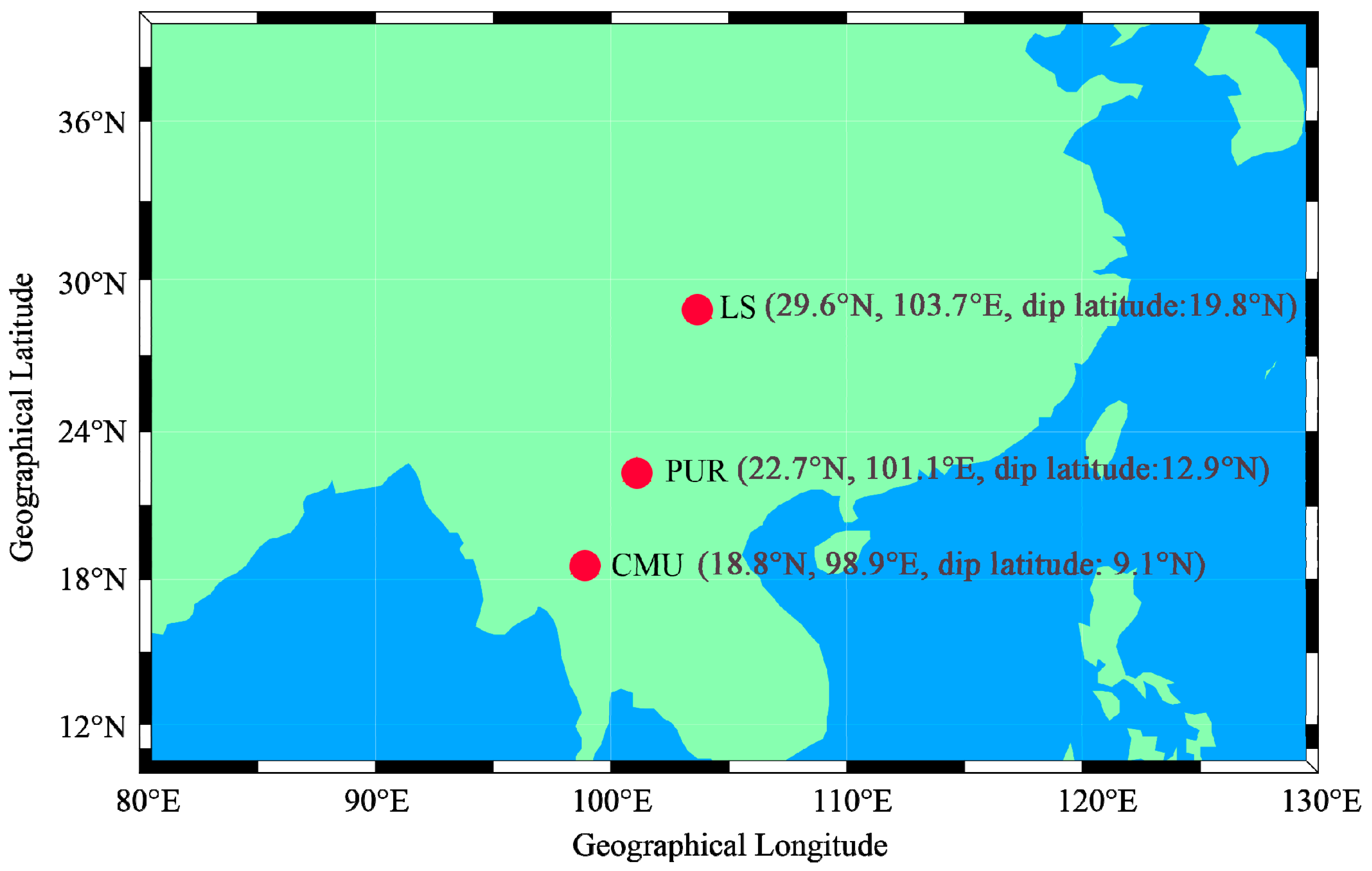
2. Instrument and Dataset
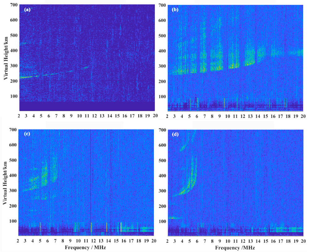
We analyzed ionograms recorded at intervals of five minutes from three ionosondes located at equatorial ionization anomaly (EIA) crest around 100° E longitudinal sector in 2016 during the descending phase of the 24th solar cycle. The positions of three ionosondes are Chiang Mai (CMU), Thailand (18.8° N, 98.9° E, magnetic latitude is 9.1° N), PUR, China (22.7° N, 101.1° E, magnetic latitude is 12.9° N), and Leshan (LS), China (29.6° N, 103.7° E, magnetic latitude is 19.8° N), and are shown in Figure 1. The ionosondes at PUR and LS stations are the advanced digital ionosonde named Wuhan Ionospheric Sounding System [35]. The ionosonde at CMU station is Frequency Modulated Continuous Wave (FMCW) ionosonde [36]. In this work, about 247,255 ionograms were manually examined to study the statistical characteristics of SF occurrence. According to SF traces in the ionogram, we classified SF into four types, such as range SF (RSF), mixed SF (MSF), frequency SF (FSF), and strong range SF (SSF). A typical example of different types of SF is shown in Figure 2.

3. Results

We investigated the spatial and temporal characteristics of the SFs of different types at three different latitudes along 100° E in 2016 by using ionogram data obtained by ionosondes.
In order to study the seasonal characteristics of each type of SF, the data in 2016 were divided into three seasons: equinox (March, April, September, and October), summer (May, June, July, and August) and winter (November, December, January, and February). The occurrence rates were calculated during each time quantum. Figure 3 shows the diurnal variation in the SF occurrence rate of each type during different seasons at the three ionosonde sites in 2016. By comparing the statistical results of the three stations, it is found that the highest occurrence of SF occurred during the June solstice at all stations, and FSF is the dominant type of SF. For all stations and seasons, the maximum occurrences of RSF with 11% and SSF (if occurred) with 3.4% appeared during the post-sunset hours (about 19 LT–23 LT); meanwhile, the maximum occurrences of FSF with 49.2% and MSF with 25% were at around midnight (about 24 LT) or post-midnight (about 00 LT–06 LT). The RSF and SSF occurrence decreased with increasing latitude, and they almost disappeared at the latitude of the LS station; in contrast, FSF occurrence increased with increasing latitude and maintained a high occurrence rate at the CMU station during the June solstice.
Figure 4 presents the occurrence rate variations of each type of SF with the month and local time. Figure 4 shows the variation trends of different types of SF with the latitudes already mentioned above. The maximum occurrence of FSF with about 60% occurred at the LS station during June, shown in Figure 4c, and RSF occurrence reached about 16% at the CMU station during March, shown in Figure 4d. Moreover, it can be seen that the RSF at the CMU station was clearly generated earlier, during the equinox, than the summer, and SSF rarely occurred in the summer.
Lan et al. [9] proposed that different types of SF event can convert to each other during the evolution process of SF, and analyzing the statistical characteristics of individual types of SF could not provide enough information to investigate the generation mechanism of SF. In order to investigate the possible linkage among the different types of SF, a series of ionograms were taken in which SF phenomenon was continually observed with time durations greater than half an hour being defined as one SF event. Because the SF type for an individual ionogram in one SF event might change, the type of SF event is marked with the SF type of the first ionogram in the SF event. Figure 5 shows the numbers of SF events for different types marked by the initial type. From Figure 5, SF events were marked by FSF as the dominant type, while only a few SSF events occurred at the CMU and PUR stations. It should be noted that the number of SF events marked by MSF decreased significantly compared with the statistical results in Figure 3 and Figure 4. For PUR station, only 29 MSF events were observed in Figure 3, which was comparable to the number of RSF events (33), while the maximum occurrence rate of the MSF events was about 2.5 times higher than that of RSF.
Figure 6 shows the time of duration of SF events marked by FSF and RSF types with day and local time. In Figure 6, it can be found that the FSF at the LS station in Figure 6c began around 19 LT and was progressively later at the lower latitude stations in Figure 6a,b. The number of FSF events lasting more than 5 h was greater in the LS station than that in the PUR and CMU stations. For RSF events, the occurrence was mostly focused on hours before midnight and lasted until post-midnight hours.

4. Discussion

In this study, we mainly analyzed the statistical features of the SF occurrence rate in the LS, PUR, and CMU stations in 2016. The statistical results showed that the SF occurrence rate varies significantly with the local time, season, latitude, and type. For RSF events, R-T instability is believed to be the main generation mechanism [9]. In Figure 3 and Figure 4, the initial time of RSF was later in the summer than that in the equinoxes in the PUR and CMU stations. The similar seasonal variation in the initial time of RSF has been observed at other low latitudes, such as Sanya station. The reason is believed to be due to the enhancement of the eastward electric field before its reversal to a westward direction at sunset that appears later in the summer [16,37]. Moreover, by comparing the occurrence rate of RSF in the three stations, it was found that the occurrence rate of RSF in CMU, which is located closest to the equator, reached the maximum value, while the occurrence rate of RSF in LS at middle latitudes was extremely low. And the RSF occurrence during the equinox was lower than that in the summer in the PUR and LS stations, which was different from the seasonal feature of RSF occurrence in the equatorial region [38,39,40], but the result agrees with many former results observed at mid-latitude [4,23,24]. Wang et al. [24] reported the statistical results of spread F observed at 10 mid-latitude stations in China and Japan, and also found the occurrence of SF activity peaks during the local summer in the Northern Hemisphere, and that RSF occurrences were far lower than FSF occurrences. At seven out of ten stations as well as three stations located beyond 40° N latitude, RSF occurrences peaked in the summer. The maxima of RSF occurrence are also found in the summer at lower mid-latitudes (<50° N), as shown by Paul et al. [23]. This is coincident with our result. Thus, the reason for the generation of RSF in the low and middle latitude regions may not be limited to irregularities related to the equatorial source, but may also be induced by other reasons, such as localized generation of F-region irregularities [18,19,20,21] or the transition from other types of SF. Stoneback [41] pointed out that there is a potential causal relationship between the observed upward drifts near midnight and ESF during the June and December solstice months of the deep solar minimum years. Sun et al. [20] proposed that electrical coupling of the MSTID and the EPB could enhance RSF. Das et al. [21] also point out that the irregularities at latitudes near the northern crest of the equatorial ionization anomaly (EIA) may be caused by MSTID.
For SSF events, the occurrence rate of SSF was high only in the equinox and almost did not occur in summer in the PUR and CMU stations, shown in Figure 3 and Figure 4. Manju et al. [42] and Wang et al. [43] showed some observational examples to confirm that plasma bubbles generated in the equatorial region can propagate to low latitudes along magnetic field lines and produce SSF and scintillation phenomena. According to the statistical results, there were six cases of SF events marked by SSF that appeared in the PUR and CMU stations on the same day with the disappearance of SSF at LS, and the initiation time of five cases was earlier in CMU than that in PUR. When the irregularities generated at the equator are raised to a higher altitude, the irregularities can extend to higher latitudes along the magnetic flux tubes. A higher altitude is needed for irregularities propagating along the geomagnetic field line to higher latitudes. Compared with CMU and PUR, the LS station is located at a higher latitude region away from the magnetic equator, so it is more difficult for equatorial origin irregularities to propagate to a higher latitude away from the equator, that is at the LS station. The above observed results demonstrated that the irregularities manifested as SSF are more likely related to the plasma bubbles generated by R-T instability in the equatorial region and propagate to higher low-latitude regions.
For FSF events, the maximum occurrence rate usually occurred after midnight in the summer at all three stations in our study, as observed by Wang et al. [24]. According to the former statistical studies of equatorial and midlatitude SF, there are some similar conclusions that RSF is the dominant type of SF during high solar activity years, which peaks pre-midnight in the equinox and that FSF is dominant in the June solstice months during low solar activity years [44,45,46], while FSF is the most observed type at lower mid-latitudes and the occurrence rate of FSF is maximized at midnight or post-midnight in the June solstice months. Paul et al. [23] indicated that the FSF occurrence was maximized in the summer at lower mid-latitudes (<50° N), but different types dominated during different solar activity years and at different stations. They suggested that the types of spread F may depend on the instabilities induced by the Es layer since the electric field in the Es layer can couple to the bottom of the F layer and initiate F layer irregularities. However, in our study, FSF is the dominant type in all three stations located at low latitude, and the Es layer might not effectively couple to the F layer and affect the generation of SF at low latitudes. Otherwise, MSTID and Perkins instability is generally accepted as one of the main mechanisms for the generation of midlatitude SF. By comparing the features of the occurrences of FSF observed at the three stations and the occurrence characteristics of nighttime MSTID proposed by some former researches [47,48], we found that FSF and nighttime MSTID occurrences had similar seasonal and local time variations, with the maximum occurrence in the summer after midnight. We proposed that FSF events may be related to ionospheric irregularity generated by plasma instability at middle latitudes. Many previous studies have suggested that nighttime MSTID plays an important role in the generation of SF at middle and even low latitudes [9,49,50]. Pimenta et al. [33] pointed out that nighttime MSTID generated in the mid-latitude region could propagate to the low-latitude region and produce SF phenomenon at night based on the observed results using an all-sky airglow imager. The statistical features of nighttime MSTID have been shown in some studies. Their results showed that nighttime MSTID at middle and low latitudes mainly occurred around midnight in the summer [48,51,52]. Chen G. Y. et al. [53] also produced statistics on the occurrence of MSTID in Hong Kong (22.2° N, 114.2° E, geomagnetic inclination 12.5° N), and showed that night MSTID mainly occurred in the summer at 22:00–03:00 LT. As the magnetic latitude of the PUR station and Hong Kong is similar, the statistical results of MSTID can be applied to the PUR region. Kil et al. [54] investigated the nighttime MSTID in middle latitudes by using electron density observations from Swarm satellites, and found the MSTID activity peaks during the June solstice in 2016 along 110° E in the Northern Hemisphere. Hines [55] suggested an inverse correlation between GWs/TIDs and neutral density, which could explain the high rate of TIDs in the June solstice. As the distance between the LS and PUR stations is about 840 km, and the mean time delay of the initial time of FSF was about 2 h in Figure 6, the calculation result shows that the velocity was about 117 m/s, so the time delay of FSF is consistent with the velocities of nighttime MSTID. Thus, the occurrence characteristics of nighttime MSTID were consistent with those of FSF at low latitudes. Moreover, considering that the occurrence of RSF in the PUR and LS stations was also the highest in the summer, it is believed that there may be a certain correlation between RSF and MSTID in the summer. For MSF events, the occurrence in Figure 3 and Figure 4 was significantly higher than the number of SF events marked by MSF in Figure 5. Thus, it can be speculated that RSF and FSF could further evolve into MSF events.

5. Conclusions

In this paper, we reported the statistical features of SF near 100° E longitude in three different latitude regions including low- and lower mid-latitude sectors. The variations in local time, season, and type for SF occurrence were shown and the possible mechanisms of different types of SF were also discussed in this work. The conclusions are summarized as follows:
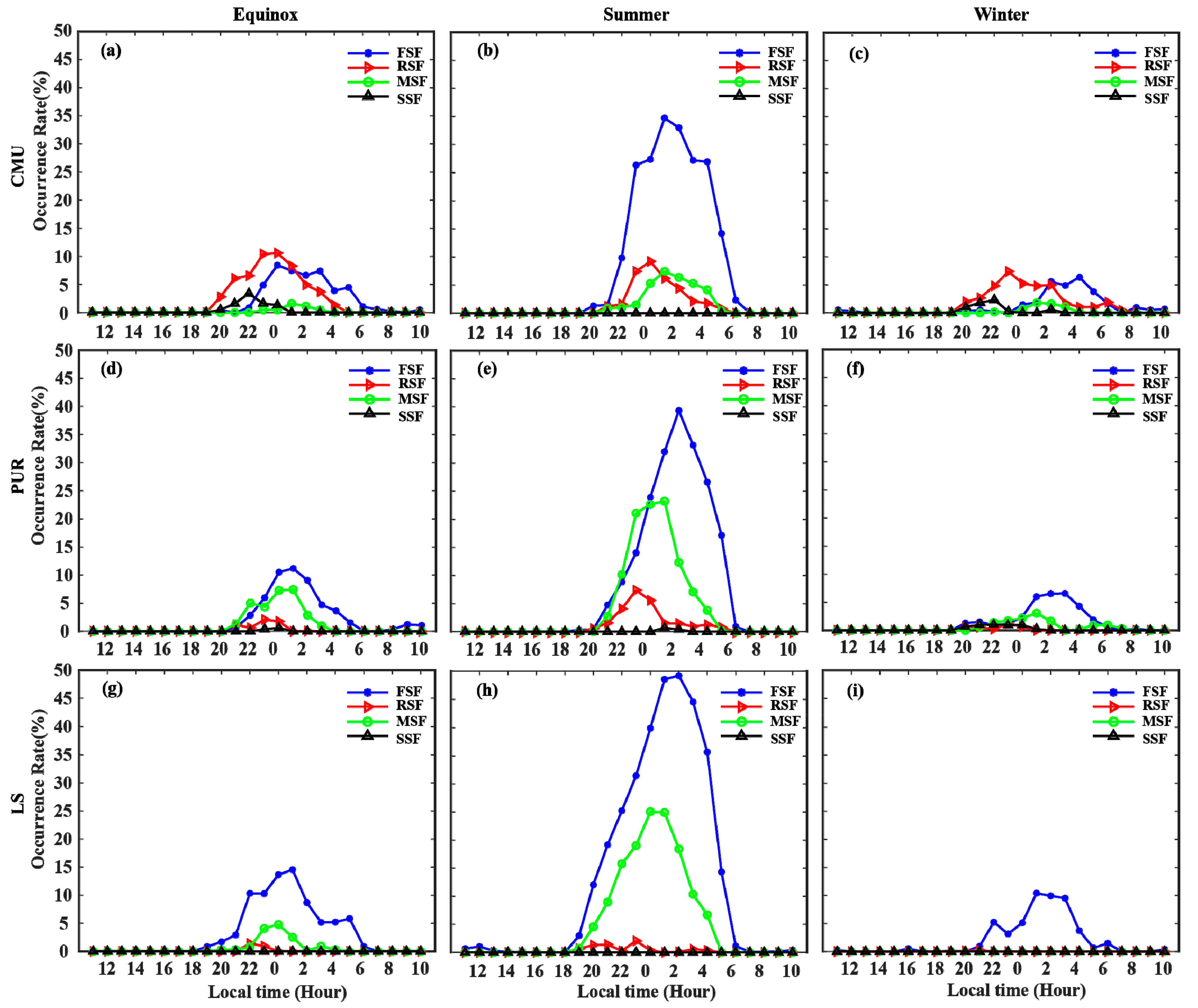
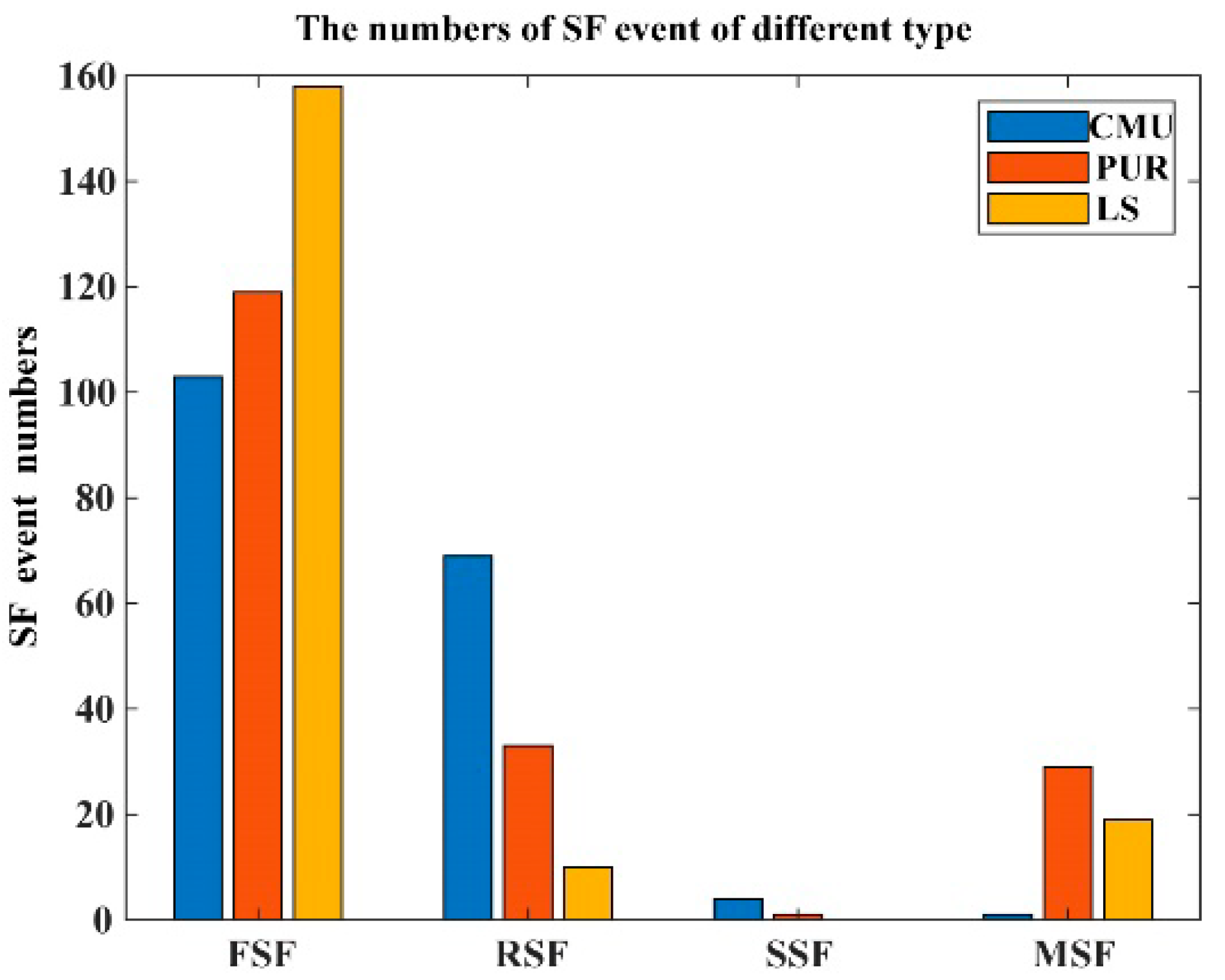
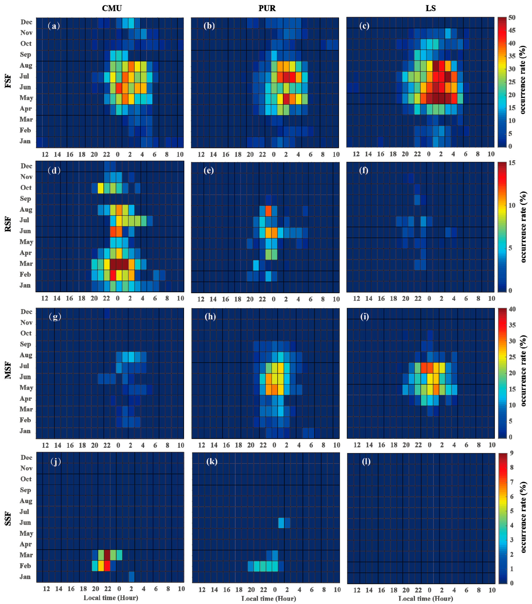
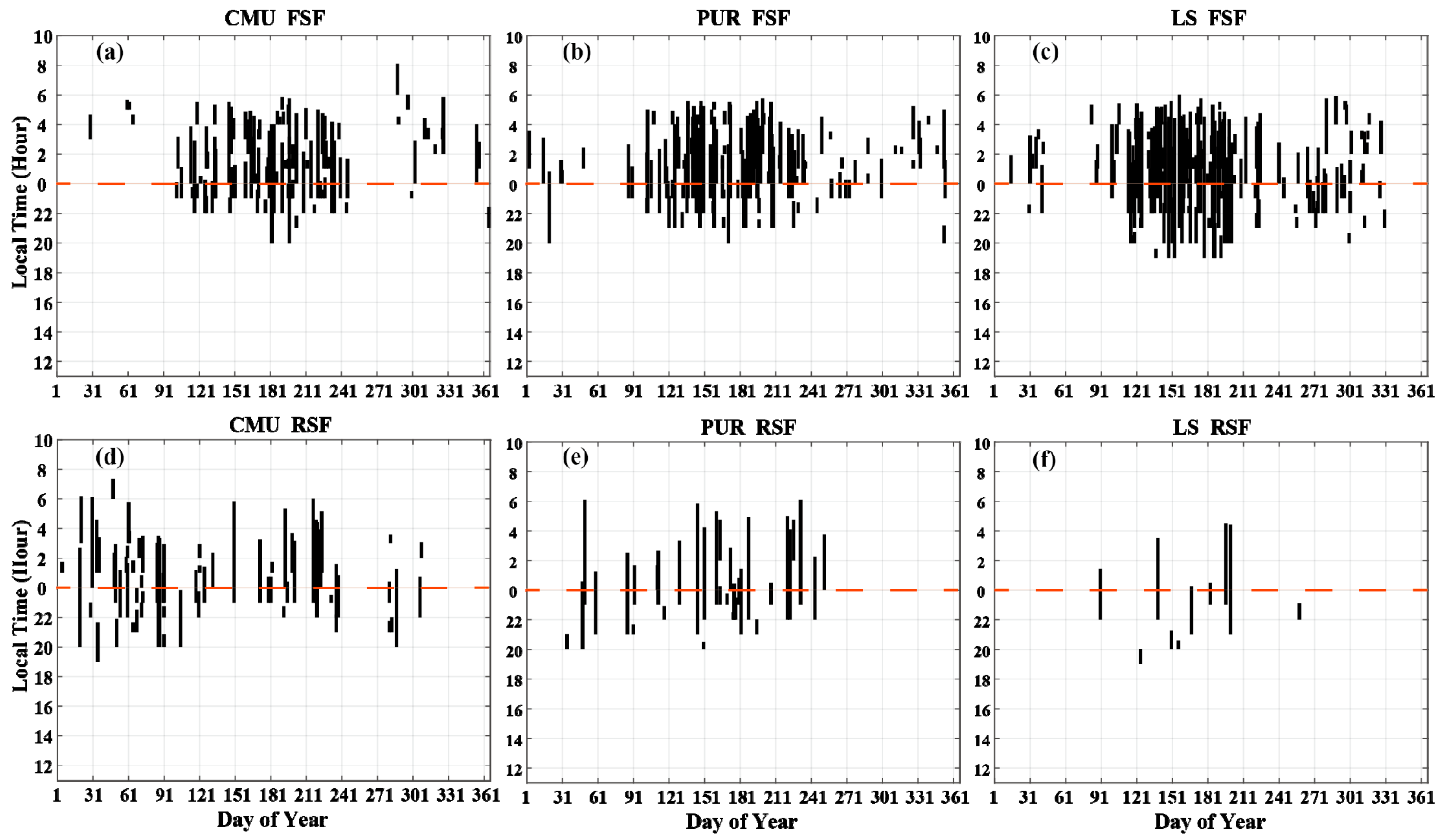
  • Our statistical results show that SF mainly occurred at night, and the RSF occurrence rate decreased with the increase in latitude at the equinox, while the FSF occurrence rate was the opposite in summer. FSF was the most prevalent type at all three stations with the maximum occurrence rate occurring after midnight, while the maximum occurrence rate of RSF and SSF occurred mainly before midnight. FSF occurred earlier at LS station and the mean time delay of the initial time of FSF among the three stations was about 2 h.
  • The importance of plasma bubbles at the equator and nighttime MSTID at middle latitudes on RSF and FSF generation has been recognized, respectively.
  • The investigation of the statistical features of SF occurrence could have a significant impact on the design and deployment of modern communication systems.

Author Contributions

Data curation, C.J. and G.Y.; methodology, C.J. and T.L.; writing—original draft preparation, T.L. and Z.X.; writing—review and editing, T.L., Z.L. and F.S. All authors have read and agreed to the published version of the manuscript.

Funding

This research was funded by the Youth Foundation of Hubei Educational Committee, Science and Technology Research Project grant number Q20202906 and Q20212904, and supported by Huanggang Normal University High-level Cultivation Project of 2021, No. 202111804.

Institutional Review Board Statement

Not applicable.

Informed Consent Statement

Not applicable.

Data Availability Statement

Ionograms recorded at CMU station are obtained from the NICT Space Weather Data and Products in Japan (http://seg-www.nict.go.jp/). The Puer and Leshan ionosonde data are available by contacting Chunhua Jiang ([email protected]).

Acknowledgments

This work is supported by the Youth Foundation of Hubei Educational Committee, Science and Technology Research Project Q20202906 and Q20212904, and supported by Huanggang Normal University High-level Cultivation Project of 2021, No. 202111804. Ionograms recorded at the CMU station were obtained from the NICT Space Weather Data and Products in Japan (http://seg-www.nict.go.jp/). The Puer and Leshan ionosonde data are available by contacting Chunhua Jiang ([email protected]). The authors acknowledge the Institute of Earthquake Forecasting for providing ionosonde data.

Conflicts of Interest

The authors declare no conflict of interest.

References

  1. Booker, H.G.; Wells, H.W. Scattering of radio waves by the F-region of the ionosphere. J. Geophys. Res. 1938, 43, 249–256. [Google Scholar] [CrossRef]
  2. Shi, J.K.; Wang, G.J.; Reinisch, B.W.; Shang, S.P.; Wang, X.; Zherebotsov, G.; Potekhin, A. Relationship between strong range spread F and ionospheric scintillations observed in Hainan from 2003 to 2007. J. Geophys. Res. 2011, 116, A08306. [Google Scholar]
  3. Bowman, G.G. A relationship between ‘‘spread-F” and the height of the F2 ionospheric layer. Aust. J. Phys. 1960, 13, 69–72. [Google Scholar] [CrossRef]
  4. Hajkowicz, L.A. Morphology of quantified ionospheric range spread-F over a wide range of midlatitudes in the Australian longitudinal sector. Ann. Geophys. 2007, 25, 1125–1130. [Google Scholar] [CrossRef]
  5. Bowman, G.G. Short-term delays (hours) of ionospheric spread F occurrence at a range of latitudes, following geomagnetic activity. J. Geophys. Res. Space Phys. 1998, 103, 11627–11634. [Google Scholar] [CrossRef]
  6. Dabas, R.S.; Das, R.M.; Sharma, K.; Garg, S.C.; Devasia, C.V.; Subbarao, K.S.V.; Rama Rao, P.V.S. Equatorial and low latitude spread-F irregularity characteristics over the Indian region and their prediction possibilities. J. Atmos. Sol. Terr. Phys. 2007, 69, 685–696. [Google Scholar] [CrossRef]
  7. Alfonsi, L.; Spogli, L.; Pezzopane, M.; Romano, V.; Zuccheretti, E.; De Franceschi, G.; Cabrera, M.A.; Ezquer, R.G. Comparative analysis of spread-F signature and GPS scintillation occurrences at Tucuman, Argentina. J. Geophys. Res. Space Phys. 2013, 118, 4483–4502. [Google Scholar] [CrossRef]
  8. Zhu, Z.P.; Lan, J.P.; Luo, W.H.; Sun, F.L.; Chen, K.; Chang, S.S. Statistical characteristics of ionogram spread-F and satellite traces over a Chinese low-latitude station Sanya. Adv. Space Res. 2015, 56, 1911–1921. [Google Scholar] [CrossRef]
  9. Lan, T.; Jiang, C.; Yang, G.; Zhang, Y.; Liu, J.; Zhao, Z. Statistical analysis of low-latitude spread F observed over Puer, China during 2015–2016. Earth Planets Space 2019, 71, 138. [Google Scholar] [CrossRef]
  10. Pimenta, A.A.; Fagundes, P.R.; Bittencourt, J.A.; Sahai, Y. Relevant aspects of equatorial plasma bubbles under different solar activity conditions. Adv. Space Res. 2001, 27, 1213–1218. [Google Scholar] [CrossRef]
  11. Sahai, Y.; Fagundes, P.R.; Bittencourt, J.A. Trans-equatorial F region ionospheric plasma bubbles: Solar cycle effects. J. Atmos. Sol. -Terr. Phys. 2000, 62, 1377–1383. [Google Scholar] [CrossRef]
  12. Abdu, M.A.; Sobral, J.H.A.; Nelson, O.R.; Batista, I.S. Solar cycle related range type spread-F occurrence characteristics over equatorial and low latitude stations in Brazil. J. Atmos. Terr. Phys. 1985, 47, 901–905. [Google Scholar] [CrossRef]
  13. Kumar, S. Morphology of equatorial plasma bubbles during low and high solar activity years over Indian sector. Astrophys. Space Sci. 2017, 362, 93. [Google Scholar] [CrossRef]
  14. Burke, W.J.; de La Beaujardière, O.; Gentile, L.C.; Hunton, D.E.; Pfaff, R.F.; Roddy, P.A.; Su, Y.J.; Wilson, G.R. C/NOFS observations of plasma density and electric field irregularities at post-midnight local times. Geophys. Res. Lett. 2009, 36, L00C09. [Google Scholar] [CrossRef]
  15. Dungey, J.W. Convective diffusion in the equatorial F region. J. Atmos. Sol. Terr. Phys. 1956, 9, 304–310. [Google Scholar] [CrossRef]
  16. Fejer, B.G.; Scherliess, L.; de Paula, E.R. Effects of the vertical plasma drift velocity on the generation and evolution of equatorial spread F. J. Geophys. Res. Space Phys. 1999, 104, 19859–19869. [Google Scholar] [CrossRef]
  17. Madhav Haridas, M.K.; Manju, G.; Arunamani, T. Solar activity variations of Equatorial Spread F occurrence and sustenance during different seasons over Indian longitudes: Empirical model and causative mechanisms. Adv. Space Res. 2018, 61, 2585–2592. [Google Scholar] [CrossRef]
  18. Li, G.; Ning, B.; Abdu, M.A.; Yue, X.; Liu, L.; Wan, W.; Hu, L. On the occurrence of post-midnight equatorial F region irregularities during the June solstice. J. Geophys. Res. 2011, 116, A04318. [Google Scholar]
  19. Zhan, W.; Rodrigues, F.; Milla, M. On the genesis of post-midnight equatorial spread F: Results for the American/Peruvian sector. Geophys. Res. Lett. 2018, 45, 7354–7361. [Google Scholar] [CrossRef]
  20. Sun, L.; Xu, J.; Zhu, Y.; Xiong, C.; Yuan, W.; Wu, K.; Hao, Y.; Chen, G.; Yan, C.; Wang, Z.; et al. Interaction between an EMSTID and an EPB in the EIA crest region over China. J. Geophys. Res. Space Phys. 2021, 126, e2020JA029005. [Google Scholar] [CrossRef]
  21. Das, T.; Paul, K.S.; Paul, A. Observation of ionospheric irregularities around midnight and post-midnight near the northern crest of the equatorial ionization anomaly in the Indian longitude sector: Case studies. J. Atmos. Sol. Terr. Phys. 2014, 121, 188–195. [Google Scholar] [CrossRef]
  22. Yokoyama, T.; Pfaff, R.F.; Roddy, P.A.; Yamamoto, M.; Otsuka, Y. On post-midnight low-latitude ionospheric irregularities during solar minimum: 2. C/NOFS observations and comparisons with the Equatorial Atmosphere Radar. J. Geophys. Res. Space Phys. 2011, 116, A11. [Google Scholar]
  23. Paul, K.S.; Haralambous, H.; Oikonomou, C.; Paul, A.; Belehaki, A.; Ioanna, T.; Kouba, D.; Buresova, D. Multi-station investigation of spread F over Europe during low to high solar activity. J. Space Weather. Space Clim. 2018, 8, A27. [Google Scholar] [CrossRef] [Green Version]
  24. Wang, N.; Guo, L.; Ding, Z.; Zhao, Z.; Xu, Z.; Xu, T.; Hu, Y. Longitudinal differences in the statistical characteristics of ionospheric spread-F occurrences at midlatitude in Eastern Asia. Earth Planets Space 2019, 71, 1–15. [Google Scholar] [CrossRef]
  25. Singleton, D.G. The morphology of spread-F occurrence over half a sunspot cycle. J. Geophys. Res. 1968, 73, 295–308. [Google Scholar] [CrossRef]
  26. Perkins, F. Spread F and ionospheric currents. J. Geophys. Res. 1973, 78, 218–226. [Google Scholar] [CrossRef]
  27. Abdu, M.A. Outstanding problems in the equatorial ionosphere–thermosphere electrodynamics relevant to spread F. J. Atmos. Sol. Terr. Phys. 2001, 63, 869–884. [Google Scholar] [CrossRef]
  28. Huang, C.S.; Miller, C.A.; Kelley, M.C. Basic properties and gravity wave initiation of the midlatitude F region instability. Radio Sci. 1994, 29, 395–405. [Google Scholar] [CrossRef]
  29. Haldoupis, C.; Kelley, M.C.; Hussey, G.C.; Shalimov, S. Role of unstable sporadic-E layers in the generation of midlatitude spread F. J. Geophys Res. 2003, 108, 2. [Google Scholar]
  30. Candido, C.M.N.; Batista, I.S.; Becker-Guedes, F.; Abdu, M.A.; Sobral, J.H.A.; Takahashi, H. Spread F occurrence over a southern anomaly crest location in Brazil during June solstice of solar minimum activity. J. Geophys. Res. 2011, 116, A06316. [Google Scholar] [CrossRef]
  31. Jiang, C.H.; Yang, G.B.; Liu, J.; Yokoyama, T.; Komolmis, T.; Song, H.; Lan, T.; Zhou, C.; Zhang, Y.N.; Zhao, Z.Y. Ionosonde observations of daytime spread F at low latitudes. J. Geophys Res. Space Phys. 2016, 121, 12093–12103. [Google Scholar] [CrossRef]
  32. Jiang, C.H.; Yang, G.B.; Liu, J.; Zhao, Z.Y. A study of the F2 layer stratifcation on ionograms using a simple model of TIDs. J. Geophys. Res. Space Phys. 2019, 124, 1317–1327. [Google Scholar] [CrossRef]
  33. Pimenta, A.A.; Kelley, M.C.; Sahai, Y.; Bittencourt, J.A.; Fagundes, P.R. Thermospheric dark band structures observed in all-sky OI 630 nm emission images over the Brazilian low-latitude sector. J. Geophys. Res. 2008, 113, A01307. [Google Scholar] [CrossRef]
  34. Krall, J.; Huba, J.D.; Ossakow, S.L.; Joyce, G.; Makela, J.J.; Miller, E.S.; Kelley, M.C. Modeling of equatorial plasma bubbles triggered by non-equatorial traveling ionospheric disturbances. Geophys. Res. Lett. 2011, 38, L08103. [Google Scholar] [CrossRef]
  35. Yao, M.; Chen, G.; Zhao, Z.; Wang, Y.; Bai, B. A novel low-power multifunctional ionospheric sounding system. IEEE Trans. Instrum. Meas. 2012, 61, 1252–1259. [Google Scholar] [CrossRef]
  36. Nozaki, K. FMCW Ionosonde for the SEALION project. J. Natl. Inst. Inf. Commun. Technol. 2009, 56, 287–298. [Google Scholar]
  37. Fejer, B.G. The electrodynamics of the low-latitude ionosphere: Recent results and future challenges. J. Atmos. Sol. Terr. Phys. 1997, 59, 1456–1482. [Google Scholar] [CrossRef]
  38. Hysell, D.L.; Burcham, J.D. Long term studies of equatorial spread F using the JULIA radar at Jicamarca. J. Atmos. Sol. Terr. Phys. 2002, 64, 1531–1543. [Google Scholar] [CrossRef]
  39. Gentile, L.C.; Burke, W.J.; Rich, F.J. A global climatology for equatorial plasma bubbles in the topside ionosphere. Ann. Geophys. 2006, 24, 163–172. [Google Scholar] [CrossRef]
  40. Rangaswamy, S.; Kapasi, K.B. Equatorial spread-F and solar activity. J. Atmos. Terr. Phys. 1964, 26, 871–878. [Google Scholar] [CrossRef]
  41. Stoneback, R.A.; Heelis, R.A.; Burrell, A.G.; Coley, W.R.; Fejer, B.G.; Pacheco, E. Observations of quiet time vertical ion drift in the equatorial ionosphere during the solar minimum period of 2009. J. Geophys. Res. 2011, 116, A12327. [Google Scholar] [CrossRef]
  42. Manju, G.; Sreeja, V.; Ravindran, S.; Thampi, S.V. Toward prediction of L band scintillations in the equatorial ionization anomaly region. J. Geophys. Res. Space Phys. 2011, 116, 307–315. [Google Scholar] [CrossRef]
  43. Wang, G.J.; Shi, J.K.; Reinisch, B.W.; Wang, X.; Wang, Z. Ionospheric plasma bubbles observed concurrently by multi-instruments over low-latitude station Hainan. J. Geophys. Res. Space Phys. 2015, 120, 2288–2298. [Google Scholar] [CrossRef]
  44. Cherniak, I.; Zakharenkova, I. First observations of super plasma bubbles in Europe. Geophys. Res. Lett. 2016, 43, 11137–11145. [Google Scholar] [CrossRef]
  45. Huang, C.-S.; de La Beaujardiere, O.; Pfaff, R.F.; Retterer, J.M.; Roddy, P.A.; Hunton, D.E.; Su, Y.-J.; Su, S.-Y.; Rich, F.J. Zonal drift of plasma particles inside equatorial plasma bubbles and its relation to the zonal drift of the bubble structure. J. Geophys. Res. 2010, 115, A07316. [Google Scholar] [CrossRef]
  46. Sastri, J.H. Letter to the Editor: Post-midnight onset of spread-F at Kodaikanal during the June solstice of solar minimum. Ann. Geophys. 1999, 17, 1111–1115. [Google Scholar]
  47. Heelis, R.A.; Stoneback, R.; Earle, G.D.; Haaser, R.A.; Abdu, M.A. Medium-scale equatorial plasma irregularities observed by coupled ion-neutral dynamics investigation sensors aboard the communication navigation outage forecast system in a prolonged solar-minimum. J. Geophys. Res. 2010, 115, A10321. [Google Scholar] [CrossRef]
  48. Ding, F.; Wan, W.X.; Xu, G.R.; Yu, T.; Yang, G.L.; Wang, J.-S. Climatology of medium-scale traveling ionospheric disturbances observed by a GPS network in central China. J. Geophys. Res. 2011, 116, A09327. [Google Scholar] [CrossRef]
  49. Bhaneja, P.; Earle, G.D.; Bullett, T.W. Statistical analysis of midlatitude spread F using multi-station digisonde observations. J. Atmos. Sol. Terr. Phys. 2018, 167, 146–155. [Google Scholar] [CrossRef]
  50. Miller, E.S.; Makela, J.J.; Kelley, M.C. Seeding of equatorial plasma depletions by polarization electric fields from middle latitudes: Experimental evidence. Geophys. Res. Lett. 2009, 36, L18105. [Google Scholar] [CrossRef]
  51. Candido, C.M.N.; Pimenta, A.A.; Bittencourt, J.A.; Becker-Guedes, F. Statistical analysis of the occurrence of medium-scale traveling ionospheric disturbances over Brazilian low latitudes using OI 630.0 nm emission all-sky images. Geophys. Res. Lett. 2008, 35, L17105. [Google Scholar] [CrossRef]
  52. Huang, F.; Lei, J.; Dou, X.; Luan, X.; Zhong, J. Nighttime medium-scale traveling ionospheric disturbances from airglow imager and Global Navigation Satellite Systems observations. Geophys. Res. Lett. 2018, 45, 31–38. [Google Scholar] [CrossRef]
  53. Chen, G.Y.; Zhou, C.; Liu, Y.; Zhao, J.Q.; Tang, Q.; Wang, X.; Zhao, Z.Y. A statistical analysis of medium-scale traveling ionospheric disturbances during 2014–2017 using the Hong Kong CORS network. Earth Planets Space 2019, 71, 52–66. [Google Scholar] [CrossRef]
  54. Kil, H.; Paxton, L.J. Global distribution of nighttime medium-scale traveling ionospheric disturbances seen by Swarm satellites. Geophys. Res. Lett. 2017, 44, 9176–9182. [Google Scholar] [CrossRef]
  55. Hines, C.O. Internal atmospheric gravity waves at ionospheric heights. Can. J. Phys. 1960, 38, 1441–1481. [Google Scholar] [CrossRef]
Figure 1. The positions of three ionosondes at equatorial ionization anomaly (EIA) crest around 100° E longitudinal sector.
Universe 08 00485 g001
Figure 2. A typical example of different types of SF. (a) RSF recorded at CMU station, (b) SSF recorded at PUR station, (c) MSF recorded at LS station and (d) FSF recorded at LS station.
Universe 08 00485 g002
Figure 3. The diurnal variation in occurrence rate of each type of SF during three seasons at (ac) CMU, (df) PUR, and (gi) LS in 2016. The formula for calculating LT is LT = UT + 7 h for the longitude of 100° E.
Universe 08 00485 g003
Figure 4. The occurrence rate variations of each type of SF with month and local time (LT = UT + 7). From top to bottom, the subfigures correspond to FSF, RSF, MSF and SSF, respectively. From left side to right side, the columns correspond to CMU, PUR and LS stations, respectively. The color bars indicate the occurrence rates of each type of SF.
Universe 08 00485 g004
Figure 5. The numbers of SF events for different types marked by the initial type.
Universe 08 00485 g005
Figure 6. Comparison between annual diurnal variation in SF events marked by FSF and RSF types over CMU, PUR and LS. (ac) the annual diurnal variation of FSF events at CMU, PUR and LS, correspondingly, and (df) the annual diurnal variation of RSF events at CMU, PUR and LS, correspondingly. The black solid lines indicate the initial time of SF events and their duration time, and the red dotted lines represent the midnight of local time (0 LT).
Universe 08 00485 g006
Publisher’s Note: MDPI stays neutral with regard to jurisdictional claims in published maps and institutional affiliations.

