Article

A Preliminary Study of Large Scale Pulsar Candidate Sifting Based on Parallel Hybrid Clustering

1
School of Physics and Electronic Science, Guizhou Normal University, Guiyang 550025, China
2
CAS Key Laboratory of FAST, National Astronomical Observatories, Chinese Academy of Sciences, Beijing 100101, China
3
School of Big Data and Computer Science, Guizhou Normal University, Guiyang 550025, China
*
Author to whom correspondence should be addressed.
Universe 2022, 8(9), 461; https://doi.org/10.3390/universe8090461
Submission received: 27 July 2022 / Revised: 31 August 2022 / Accepted: 1 September 2022 / Published: 5 September 2022
(This article belongs to the Section Astroinformatics and Astrostatistics)

Abstract

:
Pulsar candidate sifting is an essential part of pulsar analysis pipelines for discovering new pulsars. To solve the problem of data mining of a large number of pulsar data using a Five-hundred-meter Aperture Spherical radio Telescope (FAST), a parallel pulsar candidate sifting algorithm based on semi-supervised clustering is proposed, which adopts a hybrid clustering scheme based on density hierarchy and the partition method, combined with a Spark-based parallel model and a sliding window-based partition strategy. Experiments on the two datasets, HTRU (The High Time-Resolution Universe Survey) 2 and AOD-FAST (Actual Observation Data from FAST), show that the algorithm can excellently identify the pulsars with high performance: On HTRU2, the Precision and Recall rates are 0.946 and 0.905, and those on AOD-FAST are 0.787 and 0.994, respectively; the running time on both datasets is also significantly reduced compared with its serial execution mode. It can be concluded that the proposed algorithm provides a feasible idea for astronomical data mining of FAST observation.

1. Introduction

Modern pulsar surveys, including High Time Resolution Universe (HTRU) [1] Parkes survey, the Green Bank Northern Celestial Cap pulsar survey (GBNCC) [2], the Five-hundred-meter Aperture Spherical (FAST) [3,4,5,6] Telescope Survey, (CRAFTS) and so on, carry on always searching for periodic signals and produce large amounts of potential candidates for study selection. However, only an exceedingly small proportion of these candidates (approximately one in ten thousand) are real pulsars due to the presence of a large amount of radio frequency interference (RFI). Thereby, it has become critical for pulsar searches to greatly decrease the retention of a lot of non-pulsar signals but not lose pulsar-like samples as much as possible.
There are two principal components in pulsar search pipelines currently. One is a signal processor, which tries to remove RFI signals from astronomical data as much as possible by effective methods [7,8,9] and optimize the search parameters, e.g., signal-to-noise ratio (S/N) detections, etc. The other is a filtering system for minimizing the labor of further observations, which selects the pulsar-like samples among the candidates by using advanced artificial intelligence techniques. This paper focuses on pulsar candidate selection for a filtering system. Thus far, the existing pulsar candidate selection methods can be divided into three categories based on the principles of the methods. The first category refers to the traditional scoring methods. Ref. [10] proposed the Pulsar Evaluation Algorithm for Candidate Extraction (PEACE), which ranked the candidates according to their scores obtained from the quantitative evaluation of their six respective features. The second category applies classifiers based on Machine Learning (ML) methods that perform better than the traditional scoring methods. Ref. [7] proposed a Straightforward Pulsar Identification using a Neural Networks classifier (SPINN) to improve the performance of Artificial Neural Networks (ANN). Ref. [11] designed an efficient pulsar candidate classifier utilizing an ML algorithm called Gaussian Hellinger Very Fast Decision Tree (GH-VFDT). Ref. [12] optimized some features in ML and developed an ensemble classifier based on five existing decision trees. More recently, Ref. [13] introduced another strategy for pulsar candidate classification involving imbalance, which utilized a reliable KNN-based approach, called the Pseudo-Nearest Centroid Neighbor rule (PNCN). Ref. [14] utilized the combination (which is called GMO SNNNNNNNNN) of self-normalization neural network, genetic algorithm and synthetic minority over-sampling to effectively improve the performance of pulsar candidate selection. These methods were designed as binary classifications, and the features used rely heavily on human experience, which has a bad impact on the classification performance of the algorithms if used unreasonably. For instance, some classifiers extracted features just from the Dispersion Measure (DM) and pulse profile curve, resulting in some RFIs being incorrectly identified as pulsars. In the third category, the diagnostic plots were utilized as the inputs into the image recognition models based on Deep Learning (DL) so that the “pulsar-like” patterns could be automatically learned from the diagnostic subplots by training the models. Ref. [15] proposed a two-layer ensemble model for the pulsar candidate selection problem of FAST, which is composed of five classifiers based on the Pulsar Image-based Classification System (PICS). Ref. [16] utilized the Deep Convolution Generative Adversarial Network (DCGAN) model for feature extraction and the Pseudo-Inverse Learning Auto-Encoder (PILAE) classifier for classification to overcome the class imbalance. More recently, a Concat Convolutional Neural Network (CCNN) was proposed to identify the candidates that are processed from FAST data, and it is an end-to-end online learning model without any intermediate labels [17]. Compared with the traditional ML classification models, these methods have better generalization ability, but they need to manually label whether each of the subplots for each training data is “pulsar-like” individually, which will lead to a lot of extra work. In addition, some hybrid models of multi-method integration proposed by some researchers have also achieved remarkable results. Ref. [15] presented a new ensemble model as further development of PICS, which utilized a ResNet structure to identify 2D subplots and Support Vector Machine (SVM) to identify a 1D subplot.
However, in the actual calculation of pulsar surveys, there is an extremely imbalanced proportion between the pulsar and non-pulsar samples, and most of the input datasets are unlabeled. As a result, a large number of training samples for the methods (including candidate signal classifiers based on supervised ML and diagnostic subplot recognition models based on supervised DL) result in a tremendous workload. Moreover, over-fitting and under-fitting also lead to the omission of real pulsar samples in the scanning process. Facing the digestion and mining of a large number of pulsar candidates, a semi-supervised Parallel Hybrid Clustering Analyzer (PHCAL) was presented to select extremely imbalanced pulsar-like samples from large-scale candidate signals. The proposed algorithm adopts a data partition strategy based on sliding window and a parallelization scheme based on the Spark model. It is tested on HTRU2 [18,19] and AOD-FAST and compared with other classifiers presented in the mentioned literature. The experimental results show that the PHCAL algorithm can ensure the efficiency of pulsar candidate sifting. Furthermore, it can cluster more meaningful classifications, not only binary classification, so that it will promote the discovery of special pulsars that could be outliers.
The paper is organized as follows: The overall algorithm is described in detail in Section 2. Section 3 illustrates the experimental results from HTRU2 and AOD-FAST with discussions. Finally, in Section 4, the conclusions are given, and the future work is proposed.

2. The Method

2.1. Idea of Hybrid Clustering

Clustering methods are widely used to deal with large-scale data mining problems. Aiming at classifying data into some homogeneous clusters based on their similarities, existing clustering methods are categorized into density-based methods, partition-based methods, hierarchical-based methods and so on. Among the various clustering methods, k-means has been widely applied as a simple and representative partition-based clustering algorithm [20]. However, its drawbacks lie in that it is only suitable for distinguishing clusters with hyperspherical distributions of data, and the clustering results are very sensitive to the initial parameters. Therefore, several extensions of the original k-means algorithm have been presented. For example, Ref. [21] presented an improved initialization scheme of k-means that makes the initial center points as far apart from each other as possible. Ref. [22] designed the K-MODES algorithm to solve the disadvantage that k-means can only deal with numerical data. Density-based methods such as the Density-Based Spatial Clustering of Applications with Noise (DBSCAN) [23] can automatically determine the number of cluster centers and identify arbitrary-shaped clusters. However, the clustering results of DBSCAN are strongly dependent on the global parameter settings, which make it unable to handle clusters with distinct density. In addition, algorithms like DBSCAN only perform a single step to calculate cluster centers and assign a cluster label for each data sample without any iteration or optimization. Subsequently, a method called Clustering by Fast Search and Find of Density Peaks (CFSFDP) was devised by [24], which assumes that cluster centers are characterized as the local density maxima far away from any points of higher density. Since CFSFDP only focuses on the points with high density that are relatively far from each other as the center point, it is easy to divide the same cluster that contains multiple high-density points into multiple clusters. To address the above drawback, a density peak clustering algorithm was proposed using global and local consistency-adjustable manifold distances (McDPC) [25]. Hierarchical-based clustering methods can be classified as being either bottom-up [26] or top-down [27] based on how hierarchical decomposition is formed. In these methods, some parameters need to be specified in advance, and the clustering results are significantly sensitive to them, which leads to a limitation of the application scope of these methods.
Table 1 lists the advantages and disadvantages of several different kinds of artificial intelligence methods for pulsar candidate selection. As can be seen in Table 1, the idea of hybrid clustering is to effectively combine the advantages of the aforementioned different clustering algorithms, which could be more suitable for the multiple shapes of data distribution. Therefore, it can further ensure the depth and stability of data mining for pulsar candidate signals compared with other kinds of methods. Similarly, the goal of the hybrid clustering scheme of PHCAL is to combine the clustering idea based on density hierarchy and partition, which will bring the following benefits: (i) The adaptability for auto-determining the cluster number and initial clustering centers on a dataset with an irregular shape distribution can be improved. (ii) Multi-center clusters can be identified, and the clusters with lower local density can be detected to a certain extent. (iii) The more stable clusters and outliers could be obtained through the similarity metric and iterative calculation. The detailed steps of this hybrid clustering scheme are described in the next section.

2.2. The Hybrid Clustering Scheme

The detailed steps of the hybrid clustering scheme PHCAL are concluded as follows:
Step 1: Data preprocessing. The feature selection and dimensionality reduction of pulsar candidate data are carried out by Principal Component Analysis (PCA) so as to obtain input datasets from a new feature space in which the feature vector is. Notice that the optional physical eigenvalues of the pulsar candidate mainly consist of pulse radiation (e.g., single peak, double peak and multi peak), period, DM, SNR, noise signal, signal ramp, the sum of incoherent power and coherent power.
Step 2: To better reflect different data structures of clusters in the clustering results, the k-nearest neighbor-based local polynomial kernel function is adopted for the density computing on an input dataset. The Mahalanobis distance between any two data points x i and x j is defined as Equation (1).
D i s i , j = ( x i x j ) T S 1 ( x i x j )
where S is a covariance matrix of multi-dimensional random variables. Then, ρ i denotes the local density of data point x i can be calculated by the k-nearest neighbor-based polynomial function, as shown in Equation (2) since the global characteristics of the polynomial function make it have a strong generalization performance.
ρ i = x j k n n ( x i ) ( x i T x j + η ) d
where η is the offset coefficient and d is the order of the polynomial. To eliminate the affect of data variation and numerical value difference, both D i s i j and ρ i are processed by dispersion standardization as follows.
D i s i , j = D i s i , j min ( D i s i , j ) max ( D i s i , j ) min ( D i s i , j )
ρ i = ρ i min ( ρ i ) max ( ρ i ) min ( ρ i )
where min ( D i s i , j ) and min ( ρ i ) denote the minimum value of D i s i , j and ρ i separately, while max ( D i s i , j ) and max ( ρ i ) denote the maximum value of them separately.
Then, outliers from all data points are removed by Equation (5), which is helpful for the selection of cluster center points. Note that there may be some outliers screened out with very small density values, which are very few in number and are marginalized in the data distribution. Moreover, they could be some special pulsars that need to be determined.
i n l i e r = x i | ρ i > ρ t h r e h o l d
In addition, δ i denotes the minimum distance between data point x i and other higher-density data points, and can be calculated according to Equation (6).
δ i = min x i , x j inlier Dis i , j ρ i max ρ inlier and ρ i > ρ j max x i , x j inlier Dis i , j ρ i = max ρ inlier and ρ i < ρ j
Step 3: A combination of the idea of density peak and hierarchy is used to divide the hierarchy of multi-density clusters so as to determine the initial cluster center points. All the values of ρ i ( x i i n l i e r ) and δ i ( δ i > δ t h r e h o l d ) can be applied to the two-dimensional decision graph, as shown in Figure 1. An interval length γ is defined to equally divide the vertical axis, which denotes δ i of data point x i . The vertical division process is named δ -cut. Similarly, another interval length θ is defined to equally divide the horizontal axis, which denotes ρ i of data point x i . The horizontal division process is named ρ -cut. In the derived decision graph, the algorithm can automatically distinguish different density levels by using the ρ -cut and then identify the representative data points in these density levels, which are further applied to obtain all micro-clusters. Finally, the micro-cluster grouping is carried out in two ways: (i) At a low density level (not at the maximum density level), the corresponding micro-clusters should be combined together into one cluster. (ii) At the maximum density level, all the identified representative data points should be selected as cluster centers if they are at the same δ level; on the contrary, they should be merged into one single cluster if they are spread across different δ levels in the same region.
Step 4: After the number of clusters, k, and the original cluster centers were determined, the k-means iteration of distance computation of Gaussian radial basis kernel (RBF) is introduced to allocate all data points and optimize the cluster centers. According to the principle of proximity, each data point x i is assigned to the nearest cluster C i , which means the distance between x i and the center point c e n t e r i is the closest. The distance computation based on the RBF function is defined as Equation (7) to improve the similarity measure between two points.
D RBF ( i , j ) = 2 1 exp x i x j 2 σ
where σ denotes the width of the kernel function. Obviously, the local characteristics and strong learning ability of the RBF function are helping realize the mapping from measure distances to a high-dimensional space. Subsequently, each cluster C i changes to C i * , and the corresponding center c e n t e r i is refreshed as c e n t e r i * according to Equation (8).
c e n t e r i * = 1 n i x j C i x j
At each iteration, the sum of squares of errors (SSE) for all data points is calculated according to Equation (9). Until the SSE value does not change compared with the last round, the program ends. Otherwise, it returns to the next refreshing cycle. The detailed flow of the hybrid clustering scheme is summarized in Figure 2.
SSE = i = 1 k x j C i * | x j center i * | 2

2.3. Data Partition Strategy for Parallelization

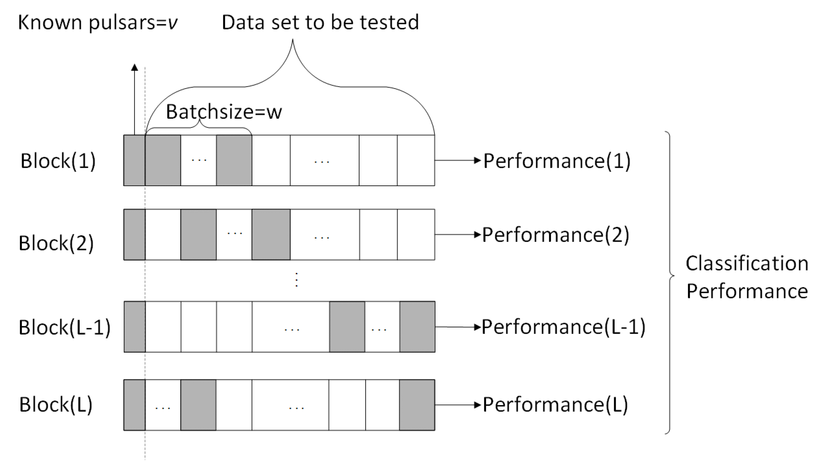
The statistics indicate that a drift scan observation with the FAST telescope can provide more than 30,000 pulsar candidates from one periodicity search (10 h or more). Furthermore, these candidates can be stored and accumulated for offline analysis and increase to a large volume over time. Hence, it is very necessary to study the parallel implementation of the hybrid clustering scheme based on parallelization models such as Mapreduce/Spark. On the one hand, a reasonable data partition strategy makes the Recall and Accuracy of the clustering results improved further; on the other hand, the time performance can also be improved by the reduction of the number of comparisons among samples.
To delineate a more comprehensive range of pulsar identification and maximize the accuracy of candidate selection based on the data structure, the sliding window concept [28] is introduced for data partitioning of candidate data streams. As shown in Figure 3, a window with Batchsize = w is delineated for each round. In addition, a relatively complete set selected from the real pulsar samples of each type is prepared and added to the data group to be detected (shadow areas) in each round in a specific ratio (v:w). At present, there is a basic assumption for clustering; that is, the samples in the same cluster are more likely to have the same markers. Therefore, the decision boundaries are set according to the dense or sparse regions of the distribution of each type of data so that the pulsar data areas and non-pulsar interference signal areas can be determined and distinguished from the derived distribution graph. By calculating the proportion of pulsar samples in each cluster, all clusters are sorted in descending order. Then, the front clusters whose proportion is greater than a certain threshold can be selected to enter a pulsar candidate list for further pulsar candidate identification. Moreover, the outliers excluded by step 2 in Section 2.2 are likely to be special pulsars, which should be further investigated. This proposed data partition strategy enables one data sample to appear in two or more blocks with a different data distribution that makes it possible for some samples incorrectly divided in one block to be correctly identified in another block, so as to further improve the overall Recall and Accuracy of the clustering results.

2.4. A Spark-Based Parallelization Model

Spark is considered a general computing engine for large-scale data processing. Therefore, a preliminary Spark-based model of PHCAL was presented, whose computing process is shown in Figure 4. The specific steps are concluded as follows.
Step 1: Carry out the parallel data partition processing, and then calculate the density value of each sample point and the Mahalanobis distance between sample points in each block. Notice that a task will be generated in each block during calculating.
Step 2: For each block, merge the corresponding micro-clusters according to step 3 in Section 2.2, and then determine the initial cluster centers.
Step 3: Traverse the initial cluster center points of each block in turn, which will be transmitted to each working node as broadcast variables in a cycle for parallel calculation.
Step 4: For the current block, read all the data points into memory if not loaded yet, then find out the nearest cluster center for each point, and then all the corresponding relationships will be collected and stored in the form of key-value pairs. Notice that M denotes the number of partitions when data are read into memory, and M is set by the system according to the hardware configuration.
Step 5: Use the map operator and aggregation operators to handle the key-value pair variables so as to update the cluster centers of the block according to step 4 in Section 2.2.
Step 6: Judge whether the distance between the new centers and their corresponding old centers is less than the set threshold. If yes, the clustering of this block is complete and move to the next block; otherwise, repeat step 4–step 6.

2.5. Time Complexity Analysis

To improve the clustering effect, the clustering scheme of PHCAL combines the idea of density hierarchy-based and partition-based clustering algorithms. Therefore, the serial clustering process of PHCAL without applying the parallelization scheme in Section 2.3 and Section 2.4 is more complex than the other three common serial classifiers, i.e., k-means++ [21], McDPC [25] and KNN [29]. However, the correct parallelization method can make up for this deficiency as much as possible. Let the number of samples in the experimental dataset be n; then Table 2 shows the time complexity of the serial mode of PHCAL compared to these three serial algorithms. (i) The time complexity of k-means++ is O n kTM . Generally, k, T and M are considered constants, so it can be simplified to O(n). (ii) For McDPC, the time complexity of computing parameters ρ and δ is O n 2 , and the time complexity of clustering based on different density levels is O n 2 , so the whole algorithm is O n 2 . (iii) The complexity of KNN is O ( n M + n D ) taken from its worst-case calculation. (iv) The complexity of the serial mode of PHCAL is O n 2 + n KTM . Since k, T and M are constants; it is simplified to O n 2 , which is close to McDPC but higher than k-means ++ and KNN. However, when running on the parallel model based on Spark, the complexity of PHCAL becomes O ( G ( p ) m ) 2 according to the Sun-Ni theorem [30], where G(p) is the factor, m is the number of samples of a block (i) and m n . Notice that when the number of parallel nodes p is sufficient (the value of p tends to reach a certain threshold for the number of divided blocks) and the communication overhead is negligible, G ( p ) 1 ; that is, the complexity is close to O m 2 .
It can be seen that the time complexity of PHCAL is obviously lower than its serial mode, in theory, if the communication delay is low enough to be ignored, which is verified by practice later. Furthermore, the speedup (Sp) and parallel efficiency (Ep) are introduced to evaluate the parallel performance of PHCAL as follows.
S p = T 1 T p = O n 2 lim G ( p ) 1 O ( G ( p ) m ) 2 , m n
T p = S p p
where T 1 denotes the running time of the serial mode, and T p denotes the running time of the parallel computing using p nodes. Generally, S p 1 , 0 E p 1 . Theoretically, the parallel performance of PHCAL will stay the same under different data sizes and hardware resources as long as the following two conditions are met. (i) The value of p is large enough (tends to reach a certain threshold); (ii) the proportion of communication delay in the running time is very small and even negligible.

3. Experiments and Results

3.1. Experimental Datasets

The HTRU2 dataset was obtained by [19] through an analysis of HTRU Medium Latitude data, which are comprised of 16,259 non-pulsar samples caused by RFI and 1639 pulsar samples. Ref. [11] made the HTRU2 dataset available. The class imbalance ratio of HTRU2 is 9.92:1. Each sample of this dataset is processed by PulsaR Exploration and Search Toolkit (PRESTO) [31] and finally designed to have eight new statistical features, including the mean value of the pulse profile, the pulse profile standard deviation, the excess kurtosis of the pulse profile, the skewness of the pulse profile, the mean value of the DM-SNR curve, the standard deviation of the DM-SNR curve, the excess kurtosis of the DM-SNR curve and the skewness of the DM-SNR curve. HTRU2 is an open telescope dataset widely used in evaluating the performance of ML algorithms.
Another dataset, AOD-FAST, is obtained from CRAFTS, which means that all the data are processed from the actual observation data of FAST. This dataset is comprised of 10,054 non-pulsar samples caused by RFI and 46 pulsar samples observed by FAST, where 46 pulsar samples are randomly mixed into the remaining non-pulsar samples. The class imbalance ratio of AOD-FAST is 218.56: 1. Notice that AODFAST adopts the same feature extraction program as that of HTRU2, which can transform the candidate data generated in the PRESTO pipeline into the input data for classification algorithms. Therefore, the data format of AOD-FAST is the same as that of HTRU2; we can perform the experiment on AOD-FAST similar to that on HTRU2. The attributes of the experimental datasets are shown in Table 3 and Table 4.

3.2. Data Preprocessing

At first, the experiment was carried out on HTRU2. From the 1639 real pulsar samples in this dataset, 1600 pulsars were randomly selected as a known sample set s, while the remaining 39 pulsars were randomly mixed into the other spurious samples to form the dataset to be detected. According to the data partition strategy in Section 2.3, the sliding window size is set to Batchsize = 2 and the unit-size is 1161, then the dataset to be detected is equally divided into t 1 , t 2 , . . . , t 13 , t 14 based on the unit-size, so that the experimental dataset is comprised of 14 data blocks, i.e., { Block ( 1 ) : s , t 1 , t 2 , Block ( 2 ) : s , t 2 , t 3 , , Block ( 13 ) : [ s , t 13 , t 14 ] , Block ( 14 ) : s , t 14 , t 1 } . Each Block(i) can be clustered separately, and when the clustering is completed, the cluster with higher pulsar sample occupancy (≥50%) will be selected for the pulsar candidate list.
Next, a similar experiment was conducted on AOD-FAST as follows. The 1639 real pulsar samples in HTRU2 were added into this dataset as a known sample set s , which changes the class imbalance ratio to 5.97:1. According to the data partition strategy, the sliding window size is set to Batchsize = 2, and the unit-size is 1010, then the original dataset is equally divided into g 1 , g 2 , . . . , g 9 , g 10 . As a result, the experimental dataset consists of 10 data blocks, i.e., { Block ( 1 ) : s , g 1 , g 2 , Block ( 2 ) : s , g 2 , g 3 , , Block ( 9 ) : s , g 9 , g 10 , Block ( 10 ) : s , g 10 , g 1 } . The subsequent clustering and class determination process are the same as that on HTRU2.
According to the flow of PHCAL, pulsar candidate data streams, regardless of their capacity, could be divided into blocks with a fixed size and processed in parallel.

3.3. Evaluation Measures

A classification algorithm is often evaluated using four metrics, i.e., Accuracy, Precision, Recall and F1-Score. Accuracy reflects the overall correctness of the algorithm, but it cannot reflect the classification performance objectively when the pulsar datasets are extremely imbalanced. Precision reflects the proportion of actual positive samples in the number of positive samples that are classified, and Recall describes the fraction of positive samples (pulsar) correctly classified. Since Precision and Recall are often contradictory for clustering, the F1-Score can be adopted to reconcile both metrics. Table 5 shows the confusion matrix of the classification.
Combined with the parallelization method in Section 2.3 and Section 2.4, the overall Precision, Recall and F1-Score are considered to evaluate the experiment, which are defined as follows:
Precision overall = 1 L l = 1 L TP l TP l + FP l
Recall l = TP l TP l + FN l ( 1 l L )
F 1 - Score overall = 1 L l = 1 L 2 × Precision l × Recall l Precision l + Recall l
Recall overall = UTP TP + FN
where L denotes the number of divided data blocks, UTP = TP 1 TP 2 TP 3 TP L denotes the union of pulsar samples identified in each data block, Recall l denotes the Recall of an individual data block while Recall overall denotes the overall Recall of the experiment.

3.4. Parameters Setting

The parameters involved in the experiment include the k-nearest neighbor points K, the threshold of density ρ t h r o h o l d , polynomial kernel parameters η and d, the RBF kernel parameter σ , the threshold for filtering small clusters δ t h r e h o l d , the ρ area division unit θ and the δ area division unit γ . The specific settings are shown in Table 6.

3.5. Clustering Effect Test

The proposed algorithm has been carried out using a Linux cluster environment with four physical computing nodes with two Intel Core i7-9700K @ 3.6 GHz CPUs, one Intel Core i7-1065G7 @ 1.5 GHz CPU and one Intel Core i5-9300H @ 2.4 GHz CPU with 32 CPU cores (68 G of total RAM, 3 T of total disk space). The system is run with centos7, Anaconda3-4.2.0, Hadoop-2.7.6 and Spark-2.3.1-bin-hadoop2.6. Each experiment was conducted for 10 rounds. Table 7 shows the classification performance of PHCAL on HTRU 2 and AOD-FAST. On HTRU2, it was compared with other supervised learning and unsupervised learning algorithms implemented on HTRU 2 in the mentioned literature. Among the unsupervised algorithms, PHCAL has the highest Precision (reaches 94.6 percent), Recall (reaches 90.5 percent) and F1-Score (reaches 88.1 percent), while the Precision, Recall and F1-Score of its serial mode are 92.2 percent, 83.5 percent (higher than k-means++ and McDPC) and 87.6 percent (also higher than k-means++ and McDpc). Compared with the supervised learning algorithms, the results of PHCAL are still good. The Recall is only lower than GMO_SNNNNNNNNN [14]; the F1-Score is lower than GMO_SNNNNNNNNN, Random Forest [32] and KNN [29] but higher than the SVM and PNCN in [13]. In addition, upon several rounds of the control test, 39 pulsar samples were randomly selected to form the dataset to be detected; it is concluded that the highest number of the pulsars detected in a round by PHCAL is 36 of 39, with an average of 34. On AOD-FAST, the Precision, Recall and F1-Score of its serial mode are 73.0 percent, 77.3 percent (higher than k-means++ and McDPC) and 75.1 percent (higher than k-means++ and McDPC), and among the 46 pulsar samples to be detected, an average of 33 can be detected in each round; the Precision, Recall and F1-Score of PHCAL are 78.7 percent, 99.4 percent and 84.6 percent, which is better at identifying pulsars. Furthermore, an average of 41 can be detected out of the 46 pulsar samples to be detected in each round.
It can be seen from Table 7 that the PHCAL ensures the clustering effect (the highest Recall) for pulsar candidate sifting on both datasets. Since it maintains the inherent advantages of semi-supervised learning and fast convergence, it is suitable for the scene of data mining of a large number of pulsar candidates. Furthermore, we believe that the clustering effect of PHCAL will be further improved with the optimization of input datasets, relevant parameters and data partition strategy in the actual pulsar search scenario.

3.6. Running Time Evaluation

To further verify the time complexity of PHCAL, the running time data were collected from the experiments. Figure 5 presents the average running time of PHCAL, compared with that of the serial mode of PHCAL, the McDPC, k-means++ and KNN mentioned in Section 2.5. Notice that PHCAL was implemented on the four-node cluster described in Section 3.5, while the serial version and other algorithms were implemented on a single computing node of the cluster above with Intel Core i7-9700K @ 3.6 GHz GPU and DDR4 3000 MHz 32 GB Memory since they cannot be implemented on a parallel structure. Moreover, the entire running time of PHCAL refers to the sum of sub-task execution time, synchronization time and communication time, excluding the time for data import. As can be seen in the figure, the serial mode of PHCAL has the longest running time, whether on HTRU2 or AOD-FAST, but the average running time of PHCAL (which is 19.23 s on HTRU2 and 12.41 s on AOD-FAST) looks much shorter compared to the others. Therefore, we get the conclusion the proposed parallel scheme of PHCAL decreases the execution time significantly while ensuring the classification performance.

4. Conclusions

A parallel hybrid clustering algorithm for large-scale pulsar candidate sifting, PHCAL, is proposed in this paper, the contributions of which are summarized as follows: (i) A hybrid clustering scheme combining the clustering idea of density hierarchy and partition was presented to ensure the clustering effect for a large number of pulsar candidates (Section 2.2). (ii) In order to better reflect different data structures of clusters in the clustering results, the k-nearest neighbor-based local polynomial kernel function was adopted for the density computing, and the local RBF kernel function was adopted for the similarity measurement between two pulsar candidate samples (Section 2.2). (iii) The sliding window-based data partition strategy and Spark-based parallelization design were introduced to further improve the correctness of the algorithm and reduce the execution time (Section 2.3 and Section 2.4). The experimental results show that PHCAL can excellently identify the pulsars with high performance (Precision and Recall) on both HTRU2 and AOD-FAST. Meanwhile, the running time on both datasets is significantly reduced compared with its serial execution mode.
Although PHCAL is proven to be feasible, it is just a preliminary research result. The clustering details and parallelization scheme need more work to be verified further. In the next step, on the one hand, the relatively complete experimental data from FAST observations will be prepared; on the other hand, the algorithm will be connected to the PRESTO-based pulsar distributed search system for practical application tests and improvements. In a word, our proposed approach has provided theoretical and practical references for sifting a large number of candidate signals observed by advanced telescopes, e.g., FAST.

Author Contributions

Conceptualization, S.-J.D., R.-S.Z. and A.-J.D.; methodology, Z.M., Z.-Y.Y., Y.L. and P.W.; software, Z.M. and S.-Y.L.; validation, Y.L. and D.-D.Z.; investigation, S.-J.D. and R.-S.Z.; writing—original draft preparation, Z.M., Z.-Y.Y. and Y.L. All authors have read and agreed to the published version of the manuscript.

Funding

This research was partially financed by the National Natural Science Fund (Nos.U1731238) and in part by the Guizhou Provincial Science and Technology Foundation (Nos.ZK[2022]304).

Institutional Review Board Statement

Not applicable.

Informed Consent Statement

Not applicable.

Data Availability Statement

Not applicable.

Acknowledgments

We would like to thank Lyon for providing datasets and feature extraction program scripts, which are very helpful to our research.

Conflicts of Interest

The authors declare no conflict of interest.

References

  1. Burke-Spolaor, S.; Bailes, M.; Johnston, S.; Bates, S.D.; Bhat, N.D.R.; Burgay, M.; D’Amico, N.; Jameson, A.; Keith, M.J.; Kramer, M.; et al. The high time resolution universe pulsar survey–iii. single-pulse searches and preliminary analysis. Mon. Not. R. Astron. Soc. 2011, 416, 2465–2476. [Google Scholar] [CrossRef]
  2. Stovall, K.; Lynch, R.S.; Ransom, S.M.; Archibald, A.M.; Banaszak, S.; Biwer, C.M.; Boyles, J.; Dartez, L.P.; Day, D.; Ford, A.J.; et al. The green bank northern celestial cap pulsar survey. I. Survey description, data analysis, and initial results. Astrophys. J. 2014, 791, 67. [Google Scholar] [CrossRef]
  3. Jiang, P.; Yue, Y.; Gan, H.; Yao, R.; Li, H.; Pan, G.; Sun, J.; Yu, D.; Liu, H.; Tang, N.; et al. Commissioning progress of the FAST. Sci. China Physics, Mech. Astron. 2019, 62, 959502. [Google Scholar] [CrossRef]
  4. Li, D.; Wang, P.; Qian, L.; Krco, M.; Dunning, A.; Jiang, P.; Yue, Y.; Jin, C.; Zhu, Y.; Pan, Z.; et al. FAST in space: Considerations for a multibeam, multipurpose survey using china’s 500-m aperture spherical radio telescope (FAST). IEEE Microw. Mag. 2018, 19, 112–119. [Google Scholar] [CrossRef]
  5. Nan, R.; Li, D.; Jin, C.; Wang, Q.; Zhu, L.; Zhu, W.; Zhang, H.; Yue, Y.; Qian, L. The five-hundred-meter aperture spherical radio telescope (FAST) project. Int. J. Mod. Phys. D 2011, 20, 989–1024. [Google Scholar] [CrossRef]
  6. Wang, P.; Li, D.; Clark, C.J.; Parkinson, P.M.S.; Hou, X.; Zhu, W.; Qian, L.; Yue, Y.; Pan, Z.; Liu, Z.; et al. FAST discovery of an extremely radio-faint millisecond pulsar from the Fermi-LAT unassociated source 3FGL J0318. 1+ 0252. Sci. China Phys. Mech. Astron. 2021, 64, 129562. [Google Scholar] [CrossRef]
  7. Morello, V.; Barr, E.D.; Bailes, M.; Flynn, C.M.; Keane, E.F.; van Straten, W. SPINN: A straightforward machine learning solution to the pulsar candidate selection problem. Mon. Not. R. Astron. Soc. 2014, 443, 1651–1662. [Google Scholar] [CrossRef]
  8. Wang, H.F.; Yuan, M.; Yin, Q.; Guo, P.; Zhu, W.W.; Li, D.; Feng, S.B. Radio frequency interference mitigation using pseudoinverse learning autoencoders. Res. Astron. Astrophys. 2020, 20, 114. [Google Scholar] [CrossRef]
  9. Yang, Z.; Yu, C.; Xiao, J.; Zhang, B. Deep residual detection of radio frequency interference for FAST. Mon. Not. R. Astron. Soc. 2020, 492, 1421–1431. [Google Scholar] [CrossRef]
  10. Lee, K.J.; Stovall, K.; Jenet, F.A.; Martinez, J.; Dartez, L.P.; Mata, A.; Lunsford, G.; Cohen, S.; Biwer, C.M.; Rohr, M.; et al. PEACE: Pulsar evaluation algorithm for candidate extraction—A software package for post-analysis processing of pulsar survey candidates. Mon. Not. R. Astron. Soc. 2013, 433, 688–694. [Google Scholar] [CrossRef]
  11. Lyon, R.J.; Stappers, B.W.; Cooper, S.; Brooke, J.M.; Knowles, J.D. Fifty years of pulsar candidate selection: From simple filters to a new principled real-time classification approach. Mon. Not. R. Astron. Soc. 2016, 459, 1104–1123. [Google Scholar] [CrossRef]
  12. Tan, C.M.; Lyon, R.J.; Stappers, B.W.; Cooper, S.; Hessels, J.W.T.; Kondratiev, V.I.; Michilli, D.; Sanidas, S. Ensemble candidate classification for the LOTAAS pulsar survey. Mon. Not. R. Astron. Soc. 2018, 474, 4571–4583. [Google Scholar] [CrossRef]
  13. Xiao, J.; Li, X.; Lin, H.; Qiu, K. Pulsar candidate selection using pseudo-nearest centroid neighbour classifier. Mon. Not. R. Astron. Soc. 2020, 492, 2119–2127. [Google Scholar] [CrossRef]
  14. Kang, Z.-W.; Liu, T.; Liu, J.; Ma, X. Pulsar candidate selection based on self-normalizing neural networks. Acta Phys. Sin. 2020, 69, 20191582. [Google Scholar] [CrossRef]
  15. Wang, H.; Zhu, W.; Guo, P.; Li, D.; Feng, S.; Yin, Q.; Miao, C.; Tao, Z.; Pan, Z.; Wang, P.; et al. Pulsar candidate selection using ensemble networks for FAST drift-scan survey. Sci. China Phys. Mech. Astron. 2019, 62, 959507. [Google Scholar] [CrossRef]
  16. Guo, P.; Duan, F.; Wang, P.; Yao, Y.; Yin, Q.; Xin, X.; Li, D.; Qian, L.; Wang, S.; Pan, Z.; et al. Pulsar candidate classification using generative adversary networks. Mon. Not. R. Astron. Soc. 2019, 490, 5424–5439. [Google Scholar] [CrossRef]
  17. Zeng, Q.; Li, X.; Lin, H. Concat Convolutional Neural Network for pulsar candidate selection. Mon. Not. R. Astron. Soc. 2020, 494, 3110–3119. [Google Scholar] [CrossRef]
  18. Lyon, R.J. Why Are Pulsars Hard to Find? The University of Manchester: Manchester, UK, 2016. [Google Scholar]
  19. Thornton, D. The High Time Resolution Radio Sky; The University of Manchester: Manchester, UK, 2013. [Google Scholar]
  20. Krishna, K.; Murty, M.N. Genetic K-means algorithm. IEEE Trans. Syst. Man Cybern. Part B (Cybernetics) 1999, 29, 433–439. [Google Scholar] [CrossRef]
  21. Vassilvitskii, S.; Arthur, D. k-means++: The advantages of careful seeding. In Proceedings of the Eighteenth Annual ACM-SIAM Symposium on Discrete Algorithms, Miami, FL, USA, 22–24 January 2006; pp. 1027–1035. [Google Scholar]
  22. Nguyen, H.H. Privacy-preserving mechanisms for k-modes clustering. Comput. Secur. 2018, 78, 60–75. [Google Scholar] [CrossRef]
  23. Simoudis, E.; Han, J.; Fayyad, U. Proceedings of the Second International Conference on Knowledge Discovery & Data Mining; AAAI Press: Menlo Park, CA, USA, 1996. [Google Scholar]
  24. Rodriguez, A.; Laio, A. Clustering by fast search and find of density peaks. Science 2014, 344, 1492–1496. [Google Scholar] [CrossRef] [Green Version]
  25. Wang, Y.; Wang, D.; Zhang, X.; Pang, W.; Miao, C.; Tan, A.H.; Zhou, Y. McDPC: Multi-center density peak clustering. Neural Comput. Appl. 2020, 32, 13465–13478. [Google Scholar] [CrossRef]
  26. Fraley, C.; Raftery, A.E. How many clusters? Which clustering method? Answers via model-based cluster analysis. Comput. J. 1998, 41, 578–588. [Google Scholar] [CrossRef]
  27. Guha, S.; Rastogi, R.; Shim, K. CURE: An efficient clustering algorithm for large databases. ACM Sigmod Rec. 1998, 27, 73–84. [Google Scholar] [CrossRef]
  28. Datar, M.; Gionis, A.; Indyk, P.; Motwani, R. Maintaining stream statistics over sliding windows. SIAM J. Comput. 2002, 31, 1794–1813. [Google Scholar] [CrossRef]
  29. Peterson, L.E. K-nearest neighbor. Scholarpedia 2009, 4, 1883. [Google Scholar] [CrossRef]
  30. Sun, X.H.; Ni, L.M. Another view on parallel speedup. In Proceedings of the 1990 ACM/IEEE Conference on Supercomputing, New York, NY, USA, 12–16 November 1990; pp. 324–333. [Google Scholar]
  31. Yue, Y.; Li, D.; Nan, R. FAST low frequency pulsar survey. Proc. Int. Astron. Union 2012, 8, 577–579. [Google Scholar] [CrossRef]
  32. Cutler, D.R.; Edwards, T.C., Jr.; Beard, K.H.; Cutler, A.; Hess, K.T.; Gibson, J.; Lawler, J.J. Random forests for classification in ecology. Ecology 2007, 88, 2783–2792. [Google Scholar] [CrossRef] [PubMed]
Figure 1. ρ and δ division of randomly generated dataset. (a) ρ division; (b) δ division.
Universe 08 00461 g001
Figure 2. Flow chart of the hybrid clustering scheme.
Universe 08 00461 g002
Figure 3. Data partition based on sliding window.
Universe 08 00461 g003
Figure 4. Computing process of Spark.
Universe 08 00461 g004
Figure 5. Average running time of PHCAL and other algorithms.
Universe 08 00461 g005
Table 1. The advantages and disadvantages of several kinds of artificial intelligence methods.
TypesMainly Represents AdvantagesDisadvantages
Empirical features-based methods[7]simple and low complexityfeatures are highly dependent on datasets
Statistical features-based methods[11,12,13]unbiased features, simple calculation, low complexity and high performancebinary classification and manually designed features
Data driving-based methods[15,16,17]data driving, avoiding manually designed features and high accuracyhigh volume of data demand, high complexity and difficult training
Clustering methods[21,22,23,24]unsupervised or semi-supervised learning and dividing more meaningful clustershighly dependent on a specific shape of data distribution
Hybrid clustering methods PHCALmore stable and suitable for the datasets of multiple shapes compared to other commonly used clustering algorithmsthe process is more complex than other commonly used clustering algorithms
Table 2. Time complexity statistics of various algorithms. T is the number of iterations, M is the characteristic number of elements, m is the number of samples of Block ( i ) , K is the number of cluster centers, and D is the nearest neighbor parameter.
AlgorithmOur AlgorithmSerial Mode of Our Algorithmk-Means++McDPCKNN
Time complexity lim G ( p ) 1 O ( G ( p ) m ) 2 O n 2 O n KTM O n 2 O n M + n D
Table 3. Basic information of both datasets used in this study. R is the class imbalance ratio of non-pulsars to pulsars.
DatasetSamplesPulsarsNon-PulsarsR
HTRU217,898163916,2599.92:1
AOD-FAST10,1004610,054218.56:1
Table 4. Details of eight statistical features designed by Lyon et al. (2016) [11].
FeatureDescription
Prof. μ Mean of the pulse profile P
Prof. σ Standard deviation of the pulse profile P
Prof.kExcess kurtosis of the pulse profile P
Prof.sSkewness of the integrated profile P
DM. μ Mean of the DM-SNR curve D
DM. σ Standard deviation of the DM-SNR curve D
DM.kExcess kurtosis of the DM-SNR curve D
DM.sSkewness of the DM-SNR curve D
Table 5. Confusion matrices.
Predicted ResultsPositiveNegative
Actual Category
TrueTPFN
FalseFPTN
Table 6. Some parameters setting of PHCAL for HTRU2 and AOD-FAST.
ParametersK ρ threhold η d σ δ threhold θ γ
Dataset
HTRU25001480.020.000050.03
AOD-FAST5001280.000010.000010.02
Table 7. Classification results with different methods for HTRU2 and AOD-FAST.
DatasetClassificationMethodPrecisionRecallF1-Score
HTRU2SupervisedSVM0.7230.9010.789
PNCN0.9230.8310.847
GMO_SNNNNNNNNN0.9550.9250.940
Random Forest0.9580.8910.921
KNN0.9520.8750.909
Unsupervised/Semi-supervisedk-means++0.9260.7470.827
McDpc0.5920.2880.388
the serial mode of PHCAL0.9220.8350.876
PHCAL0.9460.9050.881
AOD-FAST k-means++0.8370.6210.713
McDpc0.7940.6890.737
the serial mode of PHCAL0.7300.7750.751
PHCAL0.7870.9940.846
Publisher’s Note: MDPI stays neutral with regard to jurisdictional claims in published maps and institutional affiliations.

