Calculation of the Cosmological Constant for the Planetary System in Schwarzschild’s Cosmological Model

Abstract

In this work, the static cosmological model of the Schwarzschild solution for the solar system is proposed taking into account the cosmological constant in the equation of the general theory of relativity (GTR) proposed by A. Einstein. We found the nonlinear differential equation that describes the behavior of the planets around the Sun; this is solved exactly by the Jacobi and Weierstrass elliptic functions. The obtained solution allows for us to estimate the value of the cosmological constant knowing the perihelion of the different planets and from different mathematical approaches; that is, the inverse problem is solved. From the obtained results, the Schwarzschild static cosmological model for the solar system is proposed, establishing the Schwarzschild cosmological radius and the curvature limit of the solar system. From the curvature limit, different regions are proposed for the planets, exoplanets, and a region is predicted where the existence of new planets and exoplanets belonging to the solar system is possible. The proposed theory of the static Schwarzschild cosmological model may be of great interest to astronomers, cosmologists, and all those interested in the study of the universe.

1. Introduction

Albert Einstein in 1915 [1,2] formulated the general theory of gravitation (TGR), synthesizing it in the equation

$$R_{\alpha \beta }-\frac{1}{2}R{g}_{\alpha \beta }=\frac{8\pi G}{c^4}{T}_{\alpha \beta }$$

(1)

He verified that his theory explained the anomaly of the perihelion of Mercury and the curvature of light in the gravitational field of the Sun. The first exact static solution was found by Schwarzschild [3]. This solution led to deducing two great physical phenomena in our planetary system: the perihelion of the planet Mercury, the deviation of light rays in the gravitational field of the Sun, establishing that spacetime in the vicinity of a gravitational mass is curved, later experimentally demonstrated [4,5], this being a great triumph for GTG.

In the following years and recently, nonstatic solutions were found, such as those of: E. Kasner [6,7,8,9], H.P Robertson [10], A.G Walker [11], A. Friedman [12], and G. Lemaitre [13], which are called the Friedmann–Lemaitre–Robertson–Walker metric or FLRW cosmological model.

In 1917, Albert Einstein [14] could not find a static universe of his original equation. This led him to reformulate the original equation of the GTG, introducing a term called the lambda $\mathsf{\Lambda }$-cosmological constant, which encompass the physical structure of the static universe. Later, in 1937, Albert Einstein rejected this idea once De sitter [15] had established that there is a solution of Equation (1) for empty space, which represents a model of the expanding universe, and it was observed by Edwin Hubbles [16] in the redshift of galaxies, suggesting that the universe was not static, and that Eddington [17] demonstrated the expansion of the universe and that the static universe with cosmological constant was unstable [18,19].

$$R_{\alpha \beta }-\frac{1}{2}R{g}_{\alpha \beta }-\mathsf{\Lambda }{g}_{\alpha \beta }=\frac{8\pi G}{c^4}{T}_{\alpha \beta }$$

(2)

Edwin Hubbles’ discovery of the redshift, and subsequent observations of different galaxies and supernovae yielded new results that confirmed the theory of redshift, the discoveries of the radiation of the cosmic background, the acceleration of the universe, the large-scale structure of the universe, dark energy, and dark matter, leading to retaking the importance of the cosmological constant and the search for solutions to the equations proposed by A. Einstein with the cosmological constant.

Many works studied the perihelion of Mercury [20,21] and of other planets with constant zero and nonzero cosmology [22,23,24,25].

This work is organized as follows: In Section 1, Einstein’s equation is solved with the cosmological constant in vacuum with the aim that the work is complete and independent for the reader. In Section 2 are the algebraic equations of geodesics, and the nonlinear differential equation that describes the behavior of a planet around the Sun. In Section 3 and Section 4, the nonlinear differential equation is solved by means of the elliptic Jacobi functions and Weierstrass elliptic function. The cosmological constant is found as a function of the perihelion and aphelion of the planets around the Sun from different perspectives. Lastly, an exhaustive analysis of the obtained results and their consequences in Schwarzschild’s cosmological static model was carried out, for which A. Einstein so yearned and sought.

2. Solution of Einstein’s Equation with the Cosmological Constant

In this section, we propose to derive the Schwarzschild metric while taking into account the cosmological constant. For this purpose, we solve Einstein’s equation in a vacuum while taking into account the cosmological constant

$$R_{\alpha \beta }-\mathsf{\Lambda }{g}_{\alpha \beta }=0$$

(3)

where $R_{\alpha \beta }$ is the Ricci tensor, $g_{\alpha \beta }$ the metric tensor, and $\mathsf{\Lambda }$ the cosmological constant.

Since the Schwarzschild solution is static and isotropic, let us find the solution of (3) of the form:

$$d{s}^2=D\left(r\right)d{t}^2-E\left(r\right)d{r}^2-F\left(r\right)r^2(d{\theta }^2+{sin}^2\theta d{\varphi }^2)$$

(4)

Now, we perform a coordinate transformation $(ct,r,\theta ,\varphi )->(ct,\rho ,\theta ,\varphi )$ where the new coordinate $\rho$ is defined by the equation

${\rho }^2\equiv F\left(r\right)r^2$:

$$d{s}^2=A\left(\rho \right)c^{2}d{t}^2-B\left(\rho \right)d{\rho }^2-{\rho }^2(d{\theta }^2+{sin}^2\theta d{\varphi }^2)$$

(5)

The metric tensor that corresponds to the linear differential element is clearly

$$g_{\alpha \beta }=\left(\begin{array}{cccc}A\left(\rho \right)& 0& 0& 0\\ 0& -B\left(\rho \right)& 0& 0\\ 0& 0& -{\rho }^2& 0\\ 0& 0& 0& -{\rho }^2{sin}^2\theta \end{array}\right)$$

(6)

This is the metric of the more general isotropic static field problem. Functions $A\left(\rho \right)$ and $B\left(\rho \right)$ are still indeterminate, as is the relationship between coordinates $\rho$ and r. When calculating the components of Ricci tensor $R_{\alpha \beta }={\partial }_{\rho }{\mathsf{\Gamma }}_{\beta \alpha }^{\rho }-{\partial }_{\beta }{\mathsf{\Gamma }}_{\rho \alpha }^{\rho }+{\mathsf{\Gamma }}_{\rho \lambda }^{\rho }{\mathsf{\Gamma }}_{\beta \alpha }^{\lambda }-$${\mathsf{\Gamma }}_{\beta \lambda }^{\rho }{\mathsf{\Gamma }}_{\rho \alpha }^{\lambda }$, the only nonzero components are:

$$\begin{array}{c}{R}_{00}=\frac{A\left(\rho \right)\left(2B\left(\rho \right)\left(\rho A^{″}\left(\rho \right)+2A^{\prime }\left(\rho \right)\right)-\rho A^{\prime }\left(\rho \right)B^{\prime }\left(\rho \right)\right)-\rho B\left(\rho \right)A^{\prime }{\left(\rho \right)}^2}{4\rho A\left(\rho \right)B{\left(\rho \right)}^2}\\ R_{11}=\frac{A\left(\rho \right)\left(\rho A^{\prime }\left(\rho \right)+4A\left(\rho \right)\right)B^{\prime }\left(\rho \right)+\rho B\left(\rho \right)\left(A^{\prime }{\left(\rho \right)}^2-2A\left(\rho \right)A^{″}\left(\rho \right)\right)}{4\rho A{\left(\rho \right)}^{2}B\left(\rho \right)}\\ R_{22}=\frac{-\rho B\left(\rho \right)A^{\prime }\left(\rho \right)+\rho A\left(\rho \right)B^{\prime }{\left(\rho \right)}^2-2A\left(\rho \right)B\left(\rho \right)}{2A\left(\rho \right)B{\left(\rho \right)}^2}\\ R_{33}=\frac{{sin}^2\left(\varphi \right)\left(A\left(\rho \right)\left(\rho B^{\prime }{\left(\rho \right)}^2-2B\left(\rho \right)\right)-\rho B\left(\rho \right)A^{\prime }\left(\rho \right)\right)}{2A\left(\rho \right)B{\left(\rho \right)}^2}\end{array}$$

(7)

Replacing (7) and (6) in (3), we obtain the following system of equations for $A\left(\rho \right)$ end $B\left(\rho \right)$:

$$\begin{array}{c}2\rho A\left(\rho \right)B\left(\rho \right)A^{″}\left(\rho \right)-\rho A\left(\rho \right)A^{\prime }\left(\rho \right)B^{\prime }\left(\rho \right)-\rho B\left(\rho \right)A^{\prime }{\left(\rho \right)}^2+4A\left(\rho \right)B\left(\rho \right)A^{\prime }{\left(\rho \right)}^{2}B{\left(\rho \right)}^2+\mathsf{\Lambda }A\left(\rho \right)=0\\ -2\rho A\left(\rho \right)B\left(\rho \right)A^{″}\left(\rho \right)+\rho A\left(\rho \right)A^{\prime }\left(\rho \right)B^{\prime }\left(\rho \right)+\rho B\left(\rho \right)A^{\prime }{\left(\rho \right)}^2+4A{\left(\rho \right)}^2{B^{\prime }}^{2}B{\left(\rho \right)}^2-\mathsf{\Lambda }B\left(\rho \right)=0\\ -\rho B\left(\rho \right)A^{\prime }\left(\rho \right)+\rho A\left(\rho \right)B^{\prime }{\left(\rho \right)}^{2}A\left(\rho \right)B{\left(\rho \right)}^2+2A\left(\rho \right)B{\left(\rho \right)}^2-2A\left(\rho \right)B\left(\rho \right)-\mathsf{\Lambda }{\rho }^2=0\\ -{sin}^2\left(\varphi \right)\left(\rho B\left(\rho \right)A^{\prime }\left(\rho \right)-\rho A\left(\rho \right)B^{\prime }{\left(\rho \right)}^{2}A\left(\rho \right)B{\left(\rho \right)}^2-2A\left(\rho \right)B{\left(\rho \right)}^2+2A\left(\rho \right)B\left(\rho \right)\right)-\mathsf{\Lambda }{\rho }^2{sin}^2\left(\theta \right)=0\end{array}$$

(8)

Adding the first and second equations of System (8), we have $A\left(\rho \right)B^{\prime }\left(\rho \right)$ + $A^{\prime }\left(\rho \right)B\left(\rho \right)={\left(AB\right)}^{\prime }=0$. This means that:

$$A\left(\rho \right)B\left(\rho \right)=k_1,$$

(9)

so that $B\left(\rho \right)=\frac{k_1}{A\left(\rho \right)}.$ By placing this equation into the third equation of System (8), we obtain:

$$\rho A^{\prime }\left(\rho \right)+A\left(\rho \right)+k_1\mathsf{\Lambda }{\rho }^2-k_1=0,$$

(10)

from where:

$$A\left(\rho \right)=k_1-\frac{1}{3}{k}_1{\rho }^2\mathsf{\Lambda }+\frac{c_1}{\rho }$$

(11)

In order to determine the values of constants $k_1$ and $c_1$, some physical condition must be used, which is achieved by studying the situation at the Newtonian limit. When $\mathsf{\Lambda }=0$, the Newtonian potential is $\mathsf{\Phi }=-\frac{GM}{r}$; therefore,

$$g_{00}=A\left(\rho \right)\simeq 1-\frac{2GM}{c^{2}r}$$

(12)

Comparing with (11), we see that $k_1=1$ and $\frac{c_1}{\rho }=-\frac{2GM}{c^{2}r}$ The set of two variables $(c_1,\rho )$ is controlled by a single equation. This means that the values of variables $(c_1,\rho )$ are undetermined. We then need to arbitrarily determine one of the variables. The most comfortable choice is $\rho =r$; consequently, $c_1$ is equal to $-\frac{2GM}{c^2}.$ Therefore, we lastly have:

$$A=\frac{1}{B}=1-\frac{1}{3}{r}^2\mathsf{\Lambda }-\frac{2GM}{c^{2}r}$$

(13)

Linear Differential Element (4) reads [15,26].

$$d{s}^2=(1-\frac{1}{3}{r}^2\mathsf{\Lambda }-\frac{2GM}{c^{2}r})c^{2}d{t}^2-{(1-\frac{1}{3}{r}^2\mathsf{\Lambda }-\frac{2GM}{c^{2}r})}^{-1}d{r}^2-r^2(d{\theta }^2+{sin}^2\theta d{\varphi }^2),$$

(14)

where

$$g_{\alpha \beta }=\left(\begin{array}{cccc}(1-\frac{1}{3}{r}^2\mathsf{\Lambda }-\frac{2GM}{c^{2}r})& 0& 0& 0\\ 0& -{(1-\frac{1}{3}{r}^2\mathsf{\Lambda }-\frac{2GM}{c^{2}r})}^{-1}& 0& 0\\ 0& 0& -r^2& 0\\ 0& 0& 0& -r^2{sin}^2\theta \end{array}\right)$$

(15)

3. Geodesic Equations and Equation of Motion

Let us consider the motion of a planet in the gravitational field of a much heavier body (the Sun). The gravitational field of the center in spherical coordinates is given by Linear Differential Element (14).

$$d{s}^2=(1-\frac{1}{3}{r}^2\mathsf{\Lambda }-\frac{s}{r})c^{2}d{t}^2-{(1-\frac{1}{3}{r}^2\mathsf{\Lambda }-\frac{s}{r})}^{-1}d{r}^2-r^2(d{\theta }^2+{sin}^2\theta d{\varphi }^2),$$

(16)

where $s=\frac{2GM}{c^2}$. With Metric (16), we calculate the Christoffel symbols.

$${\mathsf{\Gamma }}_{\mu \nu }^{\lambda }=\frac{1}{2}{g}^{\lambda \sigma }({\partial }_{\mu }{g}_{\sigma \nu }+{\partial }_{\nu }{g}_{\sigma \mu }-{\partial }_{\sigma }{g}_{\mu \nu })$$

(17)

The nonzero quantities are:

$$\begin{array}{ccc}{\mathsf{\Gamma }}_{01}^0={\mathsf{\Gamma }}_{10}^0=\frac{3s-2r^3\mathsf{\Lambda }}{-2\mathsf{\Lambda }{r}^4+6r^2-6sr}& {\mathsf{\Gamma }}_{00}^1=\frac{c^2(\mathsf{\Lambda }{r}^3-3r+3s)(2r^3\mathsf{\Lambda }-3s)}{18r^3}& {\mathsf{\Gamma }}_{11}^1=-{\mathsf{\Gamma }}_{01}^0\\ {\mathsf{\Gamma }}_{22}^1=\frac{r^3\mathsf{\Lambda }}{3}-r+s& {\mathsf{\Gamma }}_{33}^1=\frac{1}{3}(r^3\mathsf{\Lambda }-3r+3s){sin}^2\theta & {\mathsf{\Gamma }}_{12}^2={\mathsf{\Gamma }}_{21}^2=\frac{1}{r}\\ {\mathsf{\Gamma }}_{13}^3={\mathsf{\Gamma }}_{31}^3=\frac{1}{r}& {\mathsf{\Gamma }}_{33}^2=-cos\theta sin\theta & {\mathsf{\Gamma }}_{32}^3={\mathsf{\Gamma }}_{23}^3=cot\theta \end{array}$$

(18)

Using the equations of geodesic lines $\frac{d^2{x}^{\sigma }}{d{\tau }^2}+{\mathsf{\Gamma }}_{\mu \nu }^{\sigma }\frac{d{x}^{\mu }}{d\tau }$$\frac{d{x}^{\nu }}{d\tau }=0$ and taking into account the central symmetry of our problem, any plane through the center can, however, be chosen as the plane $\theta =\frac{\pi }{2}$, that is, the orbit can be located in any plane through the center; we obtain the algebraic equations from the geodesics:

$$\begin{array}{c}\frac{2r^{\prime }{t}^{\prime }\left(3s-2\mathsf{\Lambda }{r}^3\right)}{-2\mathsf{\Lambda }{r}^4+6r^2-6rs}+t^{″}=0.\\ \frac{c^2{\left(t^{\prime }\right)}^2\left(\mathsf{\Lambda }{r}^3-3r+3s\right)\left(2\mathsf{\Lambda }{r}^3-3s\right)}{18r^3}+{{\varphi }^{\prime }}^2\left(\frac{\mathsf{\Lambda }{r}^3}{3}-r+s\right)+r^{″}\left(k\right)-\frac{{\left(r^{\prime }\right)}^2\left(3s-2\mathsf{\Lambda }{r}^3\right)}{-2\mathsf{\Lambda }{r}^4+6r^2-6rs}=0.\\ \frac{2r^{\prime }{\varphi }^{\prime }}{r}+{\varphi }^{″}=0.\end{array}$$

(19)

From the first and third equations of (19), we obtain that:

$$t^{\prime }=\frac{Er}{3s-3r+r^3\mathsf{\Lambda }},{\varphi }^{\prime }=\frac{L}{r^2},$$

(20)

where E and L are the constants of integration that represent the effective energy of the system and the angular momentum.

Dividing (14) by $d{s}^2=c^{2}d{\tau }^2$ gives

$$1=-\frac{{r^{\prime }}^2}{c^2\left(-\frac{1}{3}\mathsf{\Lambda }r{\left(\tau \right)}^2-\frac{s}{r\left(\tau \right)}+1\right)}-\frac{r{\left(\tau \right)}^2{{\varphi }^{\prime }}^2}{c^2}+{t^{\prime }}^2\left(-\frac{1}{3}\mathsf{\Lambda }r{\left(\tau \right)}^2-\frac{s}{r\left(\tau \right)}+1\right)$$

(21)

Replacing (20) into (21):

$$-\frac{L^2}{c^{2}r{\left(\tau \right)}^2}-\frac{{r^{\prime }}^2}{c^2\left(-\frac{1}{3}\mathsf{\Lambda }r{\left(\tau \right)}^2-\frac{s}{r\left(\tau \right)}+1\right)}+\frac{E^{2}r{\left(\tau \right)}^2\left(-\frac{1}{3}\mathsf{\Lambda }r{\left(\tau \right)}^2-\frac{s}{r\left(\tau \right)}+1\right)}{{\left(\mathsf{\Lambda }r{\left(\tau \right)}^3-3r\left(\tau \right)+3s\right)}^2}-1=0$$

(22)

Applying chain rule $r^{\prime }\left(\tau \right)=\frac{dr}{d\phi }\frac{d\phi }{d\tau }$, $r^{\prime }{\left(\tau \right)}^2={\left(\frac{dr}{d\phi }\right)}^2\frac{L^2}{r^4}$,

$$-r{\left(\varphi \right)}^4\left(c^2\left({\mathrm{E}}^2-9\right)+3\mathsf{\Lambda }{L}^2\right)-3c^2\mathsf{\Lambda }r{\left(\varphi \right)}^6-9c^{2}sr{\left(\varphi \right)}^3+9L^2{r^{\prime }}^2-9L^{2}sr\left(\varphi \right)+9L^{2}r{\left(\varphi \right)}^2=0$$

(23)

Using relation $r\left(\phi \right)=\frac{1}{u\left(\phi \right)}$ and taking into account that $s=\frac{2GM}{c^2}$, we obtain that

$$-\frac{c^2{\mathrm{E}}^2}{9L^2}-\frac{2GMu{\left(\varphi \right)}^3}{c^2}-\frac{c^2\mathsf{\Lambda }}{3L^{2}u{\left(\varphi \right)}^2}+\frac{c^2}{L^2}-\frac{2GMu\left(\varphi \right)}{L^2}-\frac{\mathsf{\Lambda }}{3}+{u^{\prime }}^2+u{\left(\varphi \right)}^2=0$$

(24)

or

$$-\frac{2GMu{\left(\varphi \right)}^3}{c^2}-\frac{c^2\mathsf{\Lambda }}{3L^{2}u{\left(\varphi \right)}^2}-\frac{2GMu\left(\varphi \right)}{L^2}+{u^{\prime }}^2+u{\left(\varphi \right)}^2=\frac{c^2{\mathrm{E}}^2}{9L^2}-\frac{c^2}{L^2}+\frac{\mathsf{\Lambda }}{3}=C$$

(25)

Derivating Equation (24) after simplifying (24), we obtain the equation of motion taking into account the cosmological constant:

$$\frac{d^{2}u}{d{\varphi }^2}+u-\frac{GM}{L^2}-\frac{3GM}{c^2}{u}^2+\frac{c^2\mathsf{\Lambda }}{3L^2{u}^3}=0$$

(26)

4. Einstein Equation for Planetary Motion

Let us consider the equation

$$u^{″}\left(\varphi \right)=\frac{GM}{L^2}-u\left(\varphi \right)+\frac{3GM}{c^2}{u}^2\left(\varphi \right),u\left(0\right)=\frac{1}{P}\mathrm{and}{u}^{\prime }\left(0\right)=0.$$

(27)

If we take into account cosmological constant $\mathsf{\Lambda },$ the equation is modified by adding another term as follows:

$$u^{″}\left(\varphi \right)=\frac{GM}{L^2}-\frac{c^2\mathsf{\Lambda }}{3L^2{u}^3\left(\varphi \right)}-u\left(\varphi \right)+\frac{3GM}{c^2}{u}^2\left(\varphi \right)=0,u\left(0\right)=\frac{1}{P}\mathrm{and}{u}^{\prime }\left(0\right)=0.$$

(28)

Equations (27) and (28) may both be solved in closed form. However, Equation (28) demands inverting some hyper elliptic Abelian integral and its solution is expressed in terms of a generalized Weierstrass function, which is a difficult task. Let us solve the easier Equation (27). Let

$$u\left(\varphi \right)=\frac{1}{P}-S+S{\mathrm{cn}}^2\left(\sqrt{\lambda +\mu }\varphi ,\frac{\mu }{2(\lambda +\mu )}\right).$$

(29)

Define the residual function

$$\begin{array}{c}R\left(\varphi \right)=\alpha -u\left(\varphi \right)+\gamma u^2\left(\varphi \right)-u^{″}\left(\varphi \right),\hfill \\ \\ \alpha =\frac{GM}{L^2}=\frac{3AP(A+P)-2\gamma \left(A^2+AP+P^2\right)}{6A^2{P}^2},\gamma =\frac{3GM}{c^2}.\hfill \end{array}$$

(30)

In these formulas, A stands for the aphelion and P stands for the perihelion of the planet. Number L corresponds to the angular momentum of the planet. We have

$$\begin{array}{c}R\left(\varphi \right)=\frac{-P+P^{2}S+P^2\alpha +\gamma -2PS\gamma +P^2{S}^2\gamma -2P^{2}S\lambda -P^{2}S\mu }{P^2}-\hfill \\ \\ \frac{\left(S\right(P-2\gamma +2PS\gamma -4P\lambda \left)\right)}{P}{\mathrm{cn}}^2+S(S\gamma +3\mu ){\mathrm{cn}}^4,\hfill \\ \\ \mathrm{cn}=\mathrm{cn}\left(\sqrt{\lambda +\mu }\varphi ,\frac{\mu }{2(\lambda +\mu )}\right).\hfill \end{array}$$

(31)

Equating the coefficients of cn${}^0$, cn${}^2$, and cn${}^4$ to zero gives an algebraic system whose solution is easily obtained, as follows:

$$\begin{array}{c}\lambda =\frac{-2\gamma +2\gamma PS+P}{4P},\mu =-\frac{\gamma S}{3}.\hfill \\ \\ S=\frac{6\gamma -3P+\sqrt{-12{\gamma }^2+9P^2+12\gamma P(1-4\alpha P)}}{4\gamma P}.\hfill \end{array}$$

(32)

Then,

$$u\left(\varphi \right)=\frac{1}{P}-S+S{\mathrm{cn}}^2\left(\omega \varphi ,m\right),$$

(33)

where

$$\begin{array}{c}m=\frac{1}{2}-\frac{3(\rho +2\gamma -P)}{2(\rho -6\gamma +3P)}=\frac{2GM(A-P)}{2GM(2A+P)-A{c}^{2}P}.\hfill \\ \\ \omega =\frac{1}{2}\sqrt{\frac{P-2\gamma }{P(1+m)}} and S=\frac{1}{A}-\frac{3}{2\gamma }+\frac{2}{P}.\hfill \end{array}$$

(34)

The perihelion shift is given by

$${\mathsf{\Delta }}_{GRT}=\left(\frac{2K\left(m\right)}{\omega }-2\pi \right)·\frac{23668612128}{\pi ·\mathrm{Siederal}}\text{arc-sec}/\mathrm{cy}.$$

(35)

Here, Siederal stands for the orbit period of the planet. Since, for small $m,$

$$\frac{4K\left(m\right)}{\sqrt{\frac{P-2\gamma }{(m+1)P}}}-2\pi \approx \frac{2\pi \left(3m\sqrt{\frac{P-2\gamma }{P}}+9m-16\sqrt{\frac{P-2\gamma }{P}}+16\right)}{(16-3m)\sqrt{\frac{P-2\gamma }{P}}}$$

(36)

number ${\mathsf{\Delta }}_{GRT}$ may be approximated as follows:

$$\begin{array}{c}{\tilde{\mathsf{\Delta }}}_{GRT}=\frac{47337224256\left(8A{c}^{2}P(1-\upsilon )+GM(29A\upsilon -41A+19P\upsilon -7P)\right)}{\upsilon \left(8A{c}^{2}P-GM(29A+19P)\right)·\mathrm{Siederal}}\mathrm{arcsec}/\mathrm{cy},\hfill \\ where \upsilon =\sqrt{1-\frac{2\gamma }{P}}=\sqrt{1-\frac{6GM}{c^{2}P}}\hfill \end{array}$$

(37)

Another formula:

$${\widehat{\mathsf{\Delta }}}_{GTR}=\frac{71005836384\mu \left(c^{2}P(Q+1)+2\mu Q(Q+5)\right)}{c^4{P}^2\mathrm{Siederal}}\mathrm{arcsec}/\mathrm{century},\mu =GM,Q=\frac{P}{A}.$$

(38)

Exact Value for the Perihelion Shifts

We used the following data:

Sun’s mass: $M=1.9885469241387177397120698128813396785059276218789\times {10}^{30}$

Gravitational constant: $G=6.6738399987961360272969834\times {10}^{-11}.$

Speed of light in vacuum: $c=299792458$

The results are depicted in Table 1.

Table 1. Exact and approximate values for perihelion shifts.

Planet	${\mathsf{\Delta }}_{\mathit{GTR}}$ (Exact Value)	${\widehat{\mathsf{\Delta }}}_{\mathit{GTR}}$	$\left|{\mathsf{\Delta }}_{\mathit{GTR}}-{\tilde{\mathsf{\Delta }}}_{\mathit{GTR}}\right|$
Mercury	$42.981518799592365$	$42.98151983984209$	$1.04\times {10}^{-6}$
Venus	$8.625078587720143$	$8.625078762663101$	$1.75\times {10}^{-7}$
Earth	$3.8387718031722122$	$3.8387718587113353$	$5.55\times {10}^{-8}$
Mars	$1.3508767421610324$	$1.3508767534274582$	$1.13\times {10}^{-8}$
Jupiter	$0.062311625478272306$	$0.06231162564333644$	$1.65\times {10}^{-10}$
Saturn	$0.013688932210705418$	$0.013688932230249766$	$1.95\times {10}^{-11}$
Uranus	$0.0023848021538887348$	$0.002384802155606265$	$1.72\times {10}^{-12}$
Neptune	$0.000774085957956637$	$0.0007740859583331821$	$3.77\times {10}^{-13}$
Pluto	$0.0004175446900080054$	$0.0004175446900902417$	$8.22\times {10}^{-14}$

Using NASA data, we obtained the following values for perihelion shifts:

Figure 1 illustrates the way in which Mercury’s perihelion moves.

Figure 1. Advance of Mercury’s perihelion.

Remark 1.

Equation (27) may also be written as

$$\frac{du}{d\varphi }=\sqrt{\frac{2\gamma }{3}}\sqrt{\left(u\left(\varphi \right)-\frac{1}{A}\right)\left(\frac{1}{P}-u\left(\varphi \right)\right)\left(\frac{3}{2\gamma }-\frac{1}{A}-\frac{1}{P}-u\left(\varphi \right)\right)}.$$

(39)

Integrating it gives

$$\begin{array}{ccc}T\hfill & =& 2(\varphi (1/P)-\varphi (1/A))=\frac{4K\left(\frac{2GM(A-P)}{2GM(2A+P)-A{c}^{2}P}\right)}{\sqrt{\frac{P-2\gamma }{P\left(1+\frac{2GM(A-P)}{2GM(2A+P)-A{c}^{2}P}\right)}}}=\frac{2\sqrt{6A}K\left(\frac{A-P}{P(A{\delta }_0-1)}\right)}{\sqrt{\gamma }\sqrt{A{\delta }_0-1}},\hfill \end{array}$$

(40)

$$\begin{array}{ccc}{\delta }_0\hfill & =& \frac{3}{2\gamma }-\frac{1}{A}-\frac{1}{P}.\hfill \end{array}$$

(41)

This formula also allows for us to evaluate the perihelion shift of the planet.

Remark 2.

The solution to Equation (27) is also expressed in terms of Weierstrass elliptic function $\wp$ as follows:

$$\wp \left(\varphi \right)=\frac{1}{P}-\frac{(A-P)\left(\right[3P-4\gamma ]A-2\gamma P)}{A^{2}P(P-2\gamma )\left(1+\frac{12P}{P-2\gamma }\wp (\varphi ;g_2,g_3)\right)},$$

(42)

where

$$\begin{array}{c}{g}_2=\frac{4{\gamma }^2\left(A^2+AP+P^2\right)+3A^2{P}^2-6A\gamma P(A+P)}{36A^2{P}^2}.\hfill \\ \\ g_3=\frac{(A-2\gamma )(2\gamma -P)\left(\gamma \right(A+P)-AP)}{216A^2{P}^2}.\hfill \end{array}$$

(43)

The solution is periodic with period

$$T=2{\int }_r^{\infty }\frac{dx}{\sqrt{4x^3-g_{2}x-g_3}},$$

(44)

where r is the greatest real root to the cubic $4x^3-g_{2}x-g_3=0.$ This cubic has the following real roots:

$$\begin{array}{c}{x}_1=\frac{\gamma }{6A}-\frac{1}{12},x_2=\frac{\gamma }{6P}-\frac{1}{12},x_3=\frac{1}{6}-\frac{\gamma (A+P)}{6AP}.\hfill \end{array}$$

(45)

The greatest real root is $r=x_3$; so,

$$T=2{\int }_{x_3}^{\infty }\frac{dx}{\sqrt{4x^3-g_{2}x-g_3}}=\frac{2\sqrt{6AP}F\left({sin}^{-1}\left(\sqrt{2}\sqrt{-\frac{(A-P)\gamma }{3AP-2\gamma P-4A\gamma }}\right),\frac{2(2A+P)\gamma -3AP}{2(A-P)\gamma }\right)}{\sqrt{\gamma }\sqrt{P-A}}.$$

(46)

For Mercury (see Table 2), we have the following value from (46):

$$T-2\pi =5.018176594262513\times {10}^{-7}$$

(47)

Table 2. Planets data. From [27].

Planet	A:Apelion (m)	P:Perihelion (m)	Siederal Period	$\mathit{Q}=\frac{\mathit{P}}{\mathit{A}}$
Mercury	6981,7332,000	46,000,870,000	$87.969089$	$0.658875$
Venus	108,939,198,000	107,475,372,000	$224.69562$	$0.986563$
Earth	152,100,915,000	147,094,882,000	$365.256622$	$0.967087$
Mars	249,226,166,000	206,662,107,000	$686.99329$	$0.829215$
Jupiter	816,054,481,000	740,505,444,000	$4334.24677$	$0.907422$
Saturn	1,506,619,721,000	1,348,156,111,000	10,765.21936	$0.894822$
Uranus	3,004,984,160,000	2,735,977,617,000	30,700.24558	$0.91048$
Neptune	4,538,617,181,000	4,458,057,447,000	60,226.53638	$0.98225$
Pluto	7,377,158,662,000	7,437,141,859,000	90,631.02406	$0.60147$

Remark 3.

Solution (29) may be trigonometrically approximated in as follows. We have the approximation

$$\begin{array}{c}\mathrm{cn}(t,m)\approx co{s}_m\left(t\right):=\frac{\sqrt{1+\lambda +\mu }cos\left(\sqrt{\frac{1+\lambda +\mu }{1-\mu }}t\right)}{\sqrt{1+\lambda {cos}^2\left(\sqrt{\frac{1+\lambda +\mu }{1-\mu }}t\right)+\mu {cos}^4\left(\sqrt{\frac{1+\lambda +\mu }{1-\mu }}t\right)}},\hfill \\ \\ \lambda =-\frac{1}{\mu +2}\left(m+7\mu -2m\mu -{\mu }^2+m{\mu }^2\right).\hfill \\ \\ \mu =\frac{40m^2\left(27m^2-128m+128\right)}{2409m^4-29600m^3+111520m^2-163840m+81920}.\hfill \end{array}$$

(48)

Then, the approximate trigonometric solution to I.V.P. (27) reads

$$\begin{array}{c}{u}_{\mathit{trigo}}\left(\varphi \right)=\frac{3}{2\gamma }-\frac{1}{P}-\frac{1}{A}+\left(\frac{1}{A}-\frac{3}{2\gamma }+\frac{2}{P}\right){\cos }_m^2\left(\omega \varphi \right).\hfill \\ \\ m=\frac{2GM(A-P)}{2GM(2A+P)-A{c}^{2}P},\omega =\frac{1}{2}\sqrt{\frac{P-2\gamma }{P(1+m)}},\gamma =\frac{3GM}{c^2}.\hfill \end{array}$$

(49)

Solution (49) is periodic with period

$$T_{\mathit{trigo}}=\frac{\pi }{\omega }\sqrt{\frac{1-\mu }{1+\lambda +\mu }}$$

(50)

For the Mercury data (see Table 2), we have

$${\mathsf{\Delta }}_{GRT}\approx (T_{\mathit{trigo}}-2\pi )·\frac{23668612128}{\pi ·\mathrm{Siederal}}=42.98145640188336\mathrm{arcsec}/\mathrm{cy}$$

(51)

The trigonometric solution is highly accurate.

5. Contribution of the Cosmological Constant

Let us consider I.V.P. (28). The equation may be written in the form

$$\begin{array}{c}{u}^{″}\left(\varphi \right)-\alpha +\frac{\beta }{u{\left(\varphi \right)}^3}+u\left(\varphi \right)-\gamma u{\left(\varphi \right)}^2=0,u\left(0\right)=1/P \mathrm{and} u^{\prime }\left(0\right)=0.\hfill \\ \\ \alpha =\frac{GM}{L^2},\beta =\frac{c^2\mathsf{\Lambda }}{3L^2},\gamma =\frac{3GM}{c^2}.\hfill \end{array}$$

(52)

Next, we multiply the equation $u^{″}\left(\varphi \right)-\alpha +\frac{\beta }{u{\left(\varphi \right)}^3}+u\left(\varphi \right)-\gamma u{\left(\varphi \right)}^2=0$ by $u^{\prime }\left(\varphi \right)$ and then we integrate it with regard to $\varphi$ to obtain

$$\frac{1}{2}{u}^{\prime }{\left(\varphi \right)}^2-\alpha u\left(\varphi \right)-\frac{\beta }{2u{\left(\varphi \right)}^2}-\frac{1}{3}\gamma u{\left(\varphi \right)}^3+\frac{u{\left(\varphi \right)}^2}{2}=C,$$

(53)

C is the constant of integration. Letting $\varphi =0$ and taking into account conditions $u\left(0\right)=1/P$ and $u^{\prime }\left(0\right)=0$ gives

$$C=-\frac{\gamma }{3P^3}-\frac{\beta P^2}{2}+\frac{1}{2P^2}-\frac{\alpha }{P}.$$

(54)

On the other hand, let ${\varphi }_A$ be the angle for aphelion position. Then, $u\left({\varphi }_A\right)=1/A$ and $u^{\prime }\left({\varphi }_A\right)=0$ so that

$$C=-\frac{\gamma }{3P^3}-\frac{\beta P^2}{2}+\frac{1}{2P^2}-\frac{\alpha }{P}=-\frac{\gamma }{3A^3}-\frac{A^2\beta }{2}+\frac{1}{2A^2}-\frac{\alpha }{A}.$$

(55)

From (55),

$$\alpha =\frac{GM}{L^2}=\frac{3AP(A+P)\left(A^2\beta P^2+1\right)-2\gamma \left(A^2+AP+P^2\right)}{6A^2{P}^2}.$$

(56)

The angular momentum of the planet now depends on the contribution of the cosmological constant:

$$L^2=\frac{A^2{P}^2\left(6GM-A{c}^2\mathsf{\Lambda }P(A+P)\right)}{3AP(A+P)-2\gamma \left(A^2+AP+P^2\right)}.$$

(57)

From (53)–(56),

$${\left(\frac{du}{d\varphi }\right)}^2=\frac{2\gamma \left(u-\frac{1}{A}\right)\left(\frac{1}{P}-u\right)\left(-u^3+\frac{3AP-2A\gamma -2P\gamma }{2AP\gamma }{u}^2-\frac{3AP(A+P)\beta }{2\gamma }u-\frac{3AP\beta }{2\gamma }\right)}{3u^2}$$

(58)

The solution to (58) is a periodic function with period

$$T_{\mathsf{\Lambda }}=2\sqrt{\frac{3}{2\gamma }}{\int }_{1/A}^{1/P}\frac{udu}{\sqrt{\left(u-\frac{1}{A}\right)\left(\frac{1}{P}-u\right)\left(-u^3+\frac{3AP-2A\gamma -2P\gamma }{2AP\gamma }{u}^2-\frac{3AP(A+P)\beta }{2\gamma }u-\frac{3AP\beta }{2\gamma }\right)}}.$$

(59)

6. Estimation of the Value of the Cosmological Constant

6.1. First Approach

Our aim is to find a value for $\mathsf{\Lambda }$, such that the value of $T_{\mathsf{\Lambda }}$ is as close as possible to value T given by (40). To this end, assuming a positive cosmological constant, we obtain a range for $\mathsf{\Lambda }$, say ${10}^{-k}\le \mathsf{\Lambda }\le {10}^{-m}$. Then, we evaluate (59) for $m=1,2,...,k$. We obtain a list of pairs $(j,T_{{10}^{-j}})$ that allows us to construct an interpolating function object. This function is denoted with $\mathsf{\Psi }$. The next step consists of minimizing the quantity ${(\mathsf{\Psi }\left(x\right)-T)}^2$ on the interval ${10}^{-k}\le x\le {10}^{-m}$. Let $k=56$ and $m=30$, so that ${10}^{-56}\le \mathsf{\Lambda }\le {10}^{-30}$. For Mercury data our calculations produced the optimal value ${\mathsf{\Lambda }}_{+}=4.42355\times {10}^{-44}$. On the other hand, assuming a negative cosmological constant value, we obtained the optimal value ${\mathsf{\Lambda }}_{-}=-7.41311\times {10}^{-42}$; see Table 3.

Table 3. NASA data.

	A:Apelion (m)	P:Perihelion (m)	Siederal Period	${\widehat{\mathsf{\Delta }}}_{\mathit{GTR}}$
Mercury	69.817 × 10${}^9$	46.002 × 10${}^9$	87.968	42.9814956752253
Venus	107.476 × 10${}^9$	108.939 × 10${}^9$	224.701	8.62485450672991
Earth	147.092 × 10${}^9$	152.099 × 10${}^9$	365.242	3.838987490384246
Mars	249.229 × 10${}^9$	206.617 × 10${}^9$	686.980	1.351057133139973
Jupiter	816.618 × 10${}^9$	740.522 × 10${}^9$	4332.589	0.062314275340345
Saturn	1514.504 × 10${}^9$	1352.555 × 10${}^9$	10,759.22	0.012639384845858

The confidence interval for Table 4 is:

Table 4. Estimation of the cosmological constant using the first approach.

Planet	${\mathsf{\Lambda }}_{+}$	${\mathsf{\Lambda }}_{-}$
Mercury	$6.56145\times {10}^{-38}$	$-7.94328\times {10}^{-45}$
Venus	$3.03249\times {10}^{-37}$	$-{10}^{-46}$
Earth	$4.22357\times {10}^{-38}$	$-1.2\times {10}^{-46}$
Mars	$3.8824\times {10}^{-47}$	$-3.98\times {10}^{-39}$
Jupiter	$2.02148\times {10}^{-40}$	$-1.2\times {10}^{-48}$
Saturn	$3.11889\times {10}^{-41}$	$-1.2\times {10}^{-49}$
Uranus	$3.98107\times {10}^{-42}$	$-{10}^{-50}$
Neptune	$1.58489\times {10}^{-42}$	$-1.26\times {10}^{-51}$
Pluto	$5.12861\times {10}^{-44}$	$-2.5\times {10}^{-51}$

$\begin{array}{ccc}\mathsf{\Lambda }& {\mathsf{\Lambda }}_{+}& {\mathsf{\Lambda }}_{-}\\ \mathsf{\Delta }\mathsf{\Lambda }& \left\{{-1.4\times 10}^{-37}{,2.3\times 10}^{-37}\right\}& \left\{{-1.4\times 10}^{-37}{,2.3\times 10}^{-37}\right\}\end{array}$

6.2. Second Approach

Integral (59) is hard to evaluate, so we give an approximate analytical expression. Assume a positive cosmological constant $\mathsf{\Lambda }={\mathsf{\Lambda }}_{+}$. We have

$$\begin{array}{c}-u^3+\frac{3AP-2A\gamma -2P\gamma }{2AP\gamma }{u}^2-\frac{3AP(A+P)\beta }{2\gamma }u-\frac{3AP\beta }{2\gamma }<\hfill \\ -u^3+\frac{3AP-2A\gamma -2P\gamma }{2AP\gamma }{u}^2-\frac{3AP(A+P)\beta }{2\gamma }u<\hfill \\ -u^3+\frac{3AP-2A\gamma -2P\gamma }{2AP\gamma }{u}^2-\frac{3AP(A+P)\beta }{2\gamma }{u}^2=\hfill \\ u^2({\delta }_1-u),\mathrm{where}\hfill \\ {\delta }_1=\frac{3AP-2A\gamma -2P\gamma }{2AP\gamma }-\frac{3AP(A+P)\beta }{2\gamma }.\mathrm{Then}\hfill \\ \\ \frac{u}{\sqrt{-u^3+\frac{3AP-2A\gamma -2P\gamma }{2AP\gamma }{u}^2-\frac{3AP(A+P)\beta }{2\gamma }u-\frac{3AP\beta }{2\gamma }}}>\frac{1}{\sqrt{{\delta }_1-u}}.\hfill \end{array}$$

(60)

On the other hand, since $u\ge 1/A$, $u^{-1}\le A$, $-u^{-1}\ge -A$ and $-u^{-2}\ge -A^2$, and then

$$\begin{array}{c}-u^3+\frac{3AP-2A\gamma -2P\gamma }{2AP\gamma }{u}^2-\frac{3AP(A+P)\beta }{2\gamma }u-\frac{3AP\beta }{2\gamma }=\hfill \\ u^2\left(-u+\frac{3AP-2A\gamma -2P\gamma }{2AP\gamma }-\frac{3AP(A+P)\beta }{2\gamma }{u}^{-1}-\frac{3AP\beta }{2\gamma }{u}^{-2}\right)\ge \hfill \\ u^2\left(-u+\frac{3AP-2A\gamma -2P\gamma }{2AP\gamma }-\frac{3AP(A+P)\beta }{2\gamma }A-\frac{3AP\beta }{2\gamma }{A}^2\right)=\hfill \\ u^2\left({\delta }_2-u\right),\mathrm{where}\hfill \\ {\delta }_2=\frac{3AP-2A\gamma -2P\gamma }{2AP\gamma }-\frac{3AP(A+P)\beta }{2\gamma }A-\frac{3AP\beta }{2\gamma }{A}^2.\mathrm{Then}\hfill \\ \\ \frac{u}{\sqrt{-u^3+\frac{3AP-2A\gamma -2P\gamma }{2AP\gamma }{u}^2-\frac{3AP(A+P)\beta }{2\gamma }u-\frac{3AP\beta }{2\gamma }}}\le \frac{1}{\sqrt{{\delta }_2-u}}.\hfill \end{array}$$

(61)

From (60) and (61), we obtain

$$\frac{1}{\sqrt{{\delta }_1-u}}\le \frac{u}{\sqrt{-u^3+\frac{3AP-2A\gamma -2P\gamma }{2AP\gamma }{u}^2-\frac{3AP(A+P)\beta }{2\gamma }u-\frac{3AP\beta }{2\gamma }}}<\frac{1}{\sqrt{{\delta }_2-u}},$$

(62)

Then, taking into account (59), we have estimates

$$F\left({\delta }_1\right)\le T_{{\mathsf{\Lambda }}_{+}}<F\left({\delta }_2\right),$$

(63)

where

$$F\left(\delta \right):=2\sqrt{\frac{3}{2\gamma }}{\int }_{1/A}^{1/P}\frac{du}{\sqrt{\left(u-\frac{1}{A}\right)\left(\frac{1}{P}-u\right)(\delta -u)}}=\frac{2\sqrt{6A}K\left(\frac{A-P}{P(A\delta -1)}\right)}{\sqrt{\gamma }\sqrt{A\delta -1}}.$$

(64)

Then,

$$T_{{\mathsf{\Lambda }}_{+}}\approx \frac{1}{2}(F\left({\delta }_1\right)+F\left({\delta }_2\right)).$$

(65)

Equating (40) and (65), we obtain the required equation to determine ${\mathsf{\Lambda }}_{+}$.

On the other hand, suppose that $\mathsf{\Lambda }={\mathsf{\Lambda }}_{-}$ is negative. Then, since $u>u^2$,

$$\begin{array}{c}-u^3+\frac{3AP-2A\gamma -2P\gamma }{2AP\gamma }{u}^2-\frac{3AP(A+P)\beta }{2\gamma }u-\frac{3AP\beta }{2\gamma }>\hfill \\ -u^3+\frac{3AP-2A\gamma -2P\gamma }{2AP\gamma }{u}^2-\frac{3AP(A+P)\beta }{2\gamma }u>\hfill \\ -u^3+\frac{3AP-2A\gamma -2P\gamma }{2AP\gamma }{u}^2-\frac{3AP(A+P)\beta }{2\gamma }{u}^2=\hfill \\ u^2(\frac{3AP-2A\gamma -2P\gamma }{2AP\gamma }-\frac{3AP(A+P)\beta }{2\gamma }-u)=\hfill \\ u^2({\delta }_4-u),{\delta }_4=\frac{3AP-2A\gamma -2P\gamma }{2AP\gamma }-\frac{3AP(A+P)\beta }{2\gamma }.\hfill \end{array}$$

(66)

so that

$$\frac{u}{\sqrt{-u^3+\frac{3AP-2A\gamma -2P\gamma }{2AP\gamma }{u}^2-\frac{3AP(A+P)\beta }{2\gamma }u-\frac{3AP\beta }{2\gamma }}}<\frac{1}{\sqrt{{\delta }_4-u}}$$

(67)

Now, since $u^{-1}\le A,$

$$\begin{array}{c}-u^3+\frac{3AP-2A\gamma -2P\gamma }{2AP\gamma }{u}^2-\frac{3AP(A+P)\beta }{2\gamma }u-\frac{3AP\beta }{2\gamma }=\hfill \\ u^2\left(-u+\frac{3AP-2A\gamma -2P\gamma }{2AP\gamma }-\frac{3AP(A+P)\beta }{2\gamma }{u}^{-1}-\frac{3AP\beta }{2\gamma }{u}^{-2}\right)\le \hfill \\ u^2\left(-u+\frac{3AP-2A\gamma -2P\gamma }{2AP\gamma }-\frac{3AP(A+P)\beta }{2\gamma }A-\frac{3AP\beta }{2\gamma }{A}^2\right)=\hfill \\ u^2({\delta }_3-u),where\hfill \\ {\delta }_3=\frac{3AP-2A\gamma -2P\gamma }{2AP\gamma }-\frac{3AP(A+P)\beta }{2\gamma }A-\frac{3AP\beta }{2\gamma }{A}^2.\hfill \end{array}$$

(68)

We obtained the following estimates:

$$\frac{1}{\sqrt{{\delta }_3-u}}\le \frac{u}{\sqrt{-u^3+\frac{3AP-2A\gamma -2P\gamma }{2AP\gamma }{u}^2-\frac{3AP(A+P)\beta }{2\gamma }u-\frac{3AP\beta }{2\gamma }}}$$

(69)

Using (68) and (69), and taking into account (59)–(64) we have:

$$F\left({\delta }_3\right)\le T_{{\mathsf{\Lambda }}_{-}}<F\left({\delta }_4\right).$$

(70)

The equation for ${\mathsf{\Lambda }}_{-}$ is $\frac{1}{2}(F\left({\delta }_3\right)+F\left({\delta }_4\right))=T$, where T is found from (40).

7. Approximate Analytical Solution to the Motion Equation with a Nonzero Cosmological Constant

7.1. First Solution Method

Since $\mathsf{\Lambda }$ is small,

$$u^3+\frac{3AP-2A\gamma -2P\gamma }{2AP\gamma }{u}^2-\frac{3AP(A+P)\beta }{2\gamma }u-\frac{3AP\beta }{2\gamma }\approx u^3+\frac{3AP-2A\gamma -2P\gamma }{2AP\gamma }{u}^2-\frac{3AP(A+P)\beta }{2\gamma }{u}^2.$$

(71)

Then, Hard Ode (58) may be approximated by the ode

$$\begin{array}{c}{\left(\frac{du}{d\varphi }\right)}^2=\frac{2\gamma }{3}\left(u-\frac{1}{A}\right)\left(\frac{1}{P}-u\right)\left(\delta -u\right),\mathrm{where}\hfill \\ \\ \delta =\frac{3AP-2A\gamma -2P\gamma }{2AP\gamma }-\frac{3AP(A+P)\beta }{2\gamma },\beta =\frac{c^2\mathsf{\Lambda }}{3L^2}.\hfill \\ \\ L^2=\frac{A^2{P}^2\left(6GM-A{c}^2\mathsf{\Lambda }P(A+P)\right)}{3AP(A+P)-2\gamma \left(A^2+AP+P^2\right)}.\hfill \end{array}$$

(72)

The exact solution to Ode (72) given initial conditions $u\left(0\right)=1/P$ and $u^{\prime }\left(0\right)=0$ is given by

$$u\left(\varphi \right)=\delta +\left(\frac{1}{P}-\delta \right)\mathrm{nd}{\left(\sqrt{\frac{\gamma (A\delta -1)}{6A}}\varphi ,\frac{A-P}{P(A\delta -1)}\right)}^2$$

(73)

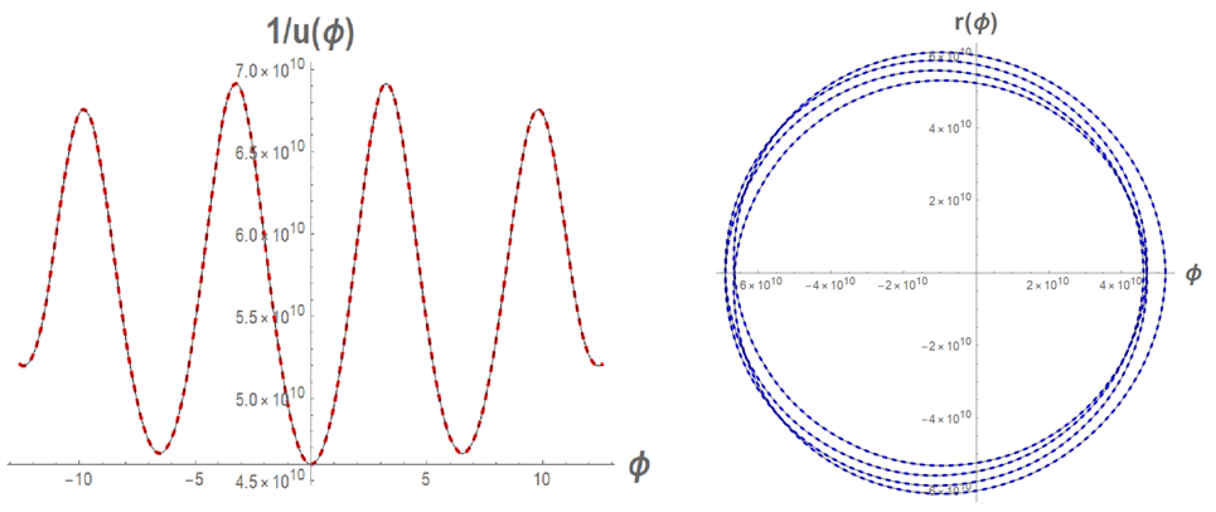
Let us compare this solution with the numerical solution to equivalent Ode (28) for Mercury data assuming the value of $\mathsf{\Lambda }={10}^{-46}$, see Figure 2.

Figure 2. Comparison between semianalytical (73) and numerical solutions to the ode.

Our semianalytical solution was highly accurate and involved the cosmological constant. This also offers another way to estimate the value of the cosmological constant. As a matter of fact, the period of the semianalytical solution reads

$$T_{\mathsf{\Lambda }}=2\frac{K\left(\frac{A-P}{P(A\delta -1)}\right)}{\sqrt{\frac{\gamma (A\delta -1)}{6A}}}$$

(74)

Then, the equation for $\mathsf{\Lambda }$ is

$$T_{\mathsf{\Lambda }}=2\sqrt{\frac{6A}{\gamma (A\delta -1)}}K\left(\frac{A-P}{P(A\delta -1)}\right)=T:=\frac{4K\left(\frac{2GM(A-P)}{A{c}^{2}P-2GM(A+2P)}\right)}{\sqrt{1-\frac{2GM(A+2P)}{A{c}^{2}P}}}$$

(75)

Since the value of $m=\frac{A-P}{P(A\delta -1)}$ is small, we may use the following approximation:

$$2K\left(m\right)\circeq \frac{1-\frac{5m}{16}}{1-\frac{9m}{16}}\pi .$$

(76)

Then,

$$T_{\mathsf{\Lambda }}=\frac{\sqrt{6}\pi \sqrt{A}(A(16\delta P-5)-11P)}{\sqrt{\gamma }\sqrt{A\delta -1}(A(16\delta P-9)-7P)}=T,$$

(77)

from where

$$\begin{array}{c}256A^3{P}^2{T}^2\gamma {\delta }^3-96A^{2}P\left(16AP{\pi }^2+3A{T}^2\gamma +5P{T}^2\gamma \right)\delta \hfill \\ +3A\left(320A^{2}P{\pi }^2+704A{P}^2{\pi }^2+27A^2{T}^2\gamma +138AP{T}^2\gamma +91P^2{T}^2\gamma \right){\delta }^2\hfill \\ -150A^3{\pi }^2-660A^{2}P{\pi }^2-726A{P}^2{\pi }^2-81A^2{T}^2\gamma -126AP{T}^2\gamma -49P^2{T}^2\gamma =0.\hfill \end{array}$$

(78)

Solving this cubic, we obtain the value for $\delta$. Then, from (72),

$$\mathsf{\Lambda }=\frac{6\mu Q^2(2\gamma \delta P-3P+2\gamma (Q+1))}{c^2{P}^2(Q+1)\left(2\gamma +2\gamma \delta P^2+2\gamma (Q+1)(P+Q)-3P(P+Q+1)\right)},Q:=\frac{P}{A}.$$

(79)

We may go further using other approximates for $K\left(m\right)$. For example,

$$K\left(m\right)\circeq \frac{\pi \left(409m^2-3984m+4864\right)}{1025m^2-5200m+4864}$$

(80)

This approximation gives us the following quintic for $\delta$:

$$C_0{\delta }^5+C_1{\delta }^4+C_2{\delta }^3+C_3{\delta }^2+C_4\delta +C_5=0,$$

(81)

where

$$C_0=23658496A^5\gamma P^4{T}^2.$$

(82)

$$C_1=-155648A^4{P}^3\left(912{\pi }^{2}AP+325A\gamma T^2+435\gamma P{T}^2\right).$$

$$C_2=256A^3{P}^2\left(908352{\pi }^2{A}^{2}P+144575A^2\gamma T^2+1309632{\pi }^{2}A{P}^2+501250A\gamma P{T}^2+278335\gamma P^2{T}^2\right).$$

(83)

$$C_3=-32A^{2}P\left(\begin{array}{c}3722064{\pi }^2{A}^{3}P+333125A^3\gamma T^2+14356320{\pi }^2{A}^2{P}^2+2470425A^2\gamma P{T}^2+\\ 8537424{\pi }^{2}A{P}^3+3544575A\gamma P^2{T}^2+1045155\gamma P^3{T}^2\end{array}\right).$$

(84)

$$C_4=A\left(\begin{array}{c}19553472{\pi }^2{A}^{4}P+1050625A^4\gamma T^2+179551680{\pi }^2{A}^3{P}^2+17117500A^3\gamma P{T}^2+279850560{\pi }^2{A}^2{P}^3+\\ 53377350A^2\gamma P^2{T}^2+88848192{\pi }^{2}A{P}^4+40032700A\gamma P^3{T}^2+6714305\gamma P^4{T}^2\end{array}\right).$$

(85)

$$\begin{array}{ccc}{C}_5\hfill & =& -1003686{\pi }^2{A}^5-15538728{\pi }^2{A}^{4}P-1050625A^4\gamma T^2-66467748{\pi }^2{A}^3{P}^2-6457500A^3\gamma P{T}^2-\hfill \\ & & 48971688{\pi }^2{A}^2{P}^3-11334950A^2\gamma P^2{T}^2-9969126{\pi }^{2}A{P}^4-4340700A\gamma P^3{T}^2-474721\gamma P^4{T}^2.\hfill \end{array}$$

(86)

Solving the quintic, we obtain one or more estimates for $\mathsf{\Lambda }$. Let us evaluate the $\mathsf{\Lambda }$ using Formula (79) for Mercury. The cubic resolvent reads

$$\begin{array}{c}-3.224134057504410567808405\times {10}^{61}{\delta }^3+1.0917240150709210311767171311214\times {10}^{58}{\delta }^2-\hfill \\ 3.6333609324359012885422051569104\times {10}^{47}\delta +3.0230424838943767016875726381236\times {10}^{36}=0.\hfill \end{array}$$

(87)

Its roots are:

$$\begin{array}{c}{\delta }_1=1.66403214678195905033219994\times {10}^{-11}.\hfill \\ {\delta }_2=1.66406282054722562545891615\times {10}^{-11}.\hfill \\ {\delta }_3=0.0003386099610925325989588409.\hfill \end{array}$$

(88)

The values of $\mathsf{\Lambda }$ from (79) are:

$${\mathsf{\Lambda }}_1=2.3818552552068309770172818\times {10}^{-29}.$$

(89)

$${\mathsf{\Lambda }}_2=2.3818552552068309770172040\times {10}^{-29}$$

(90)

$${\mathsf{\Lambda }}_3=2.574519419707803\times {10}^{-43}$$

(91)

Using the quintic, we obtain the negative value

$$\mathsf{\Lambda }=-1.0241093318102231833808\times {10}^{-47}$$

(92)

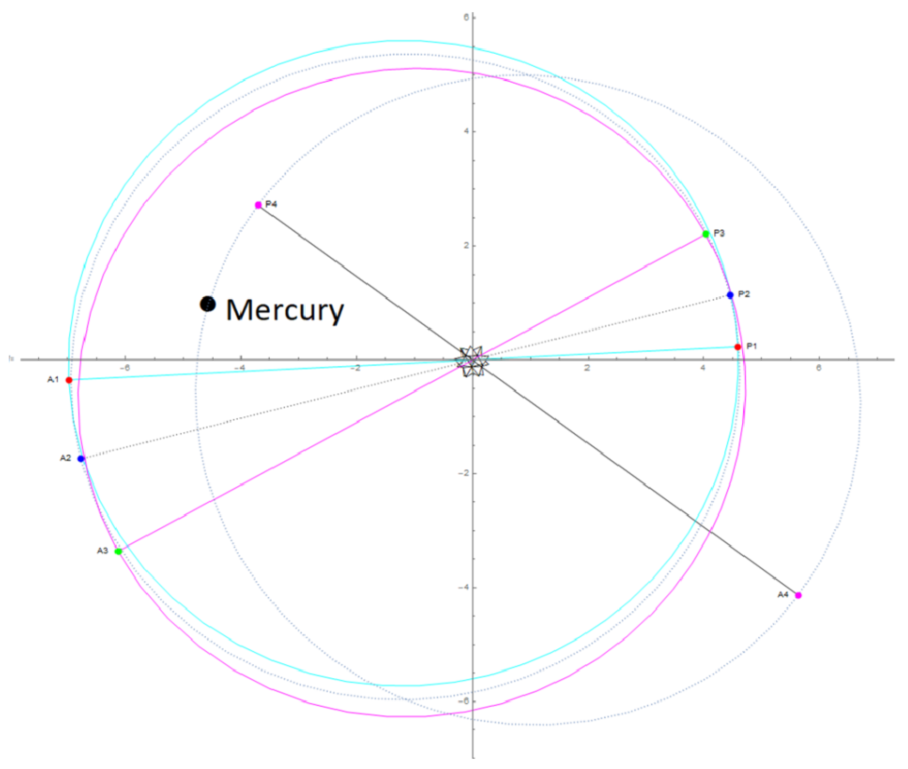
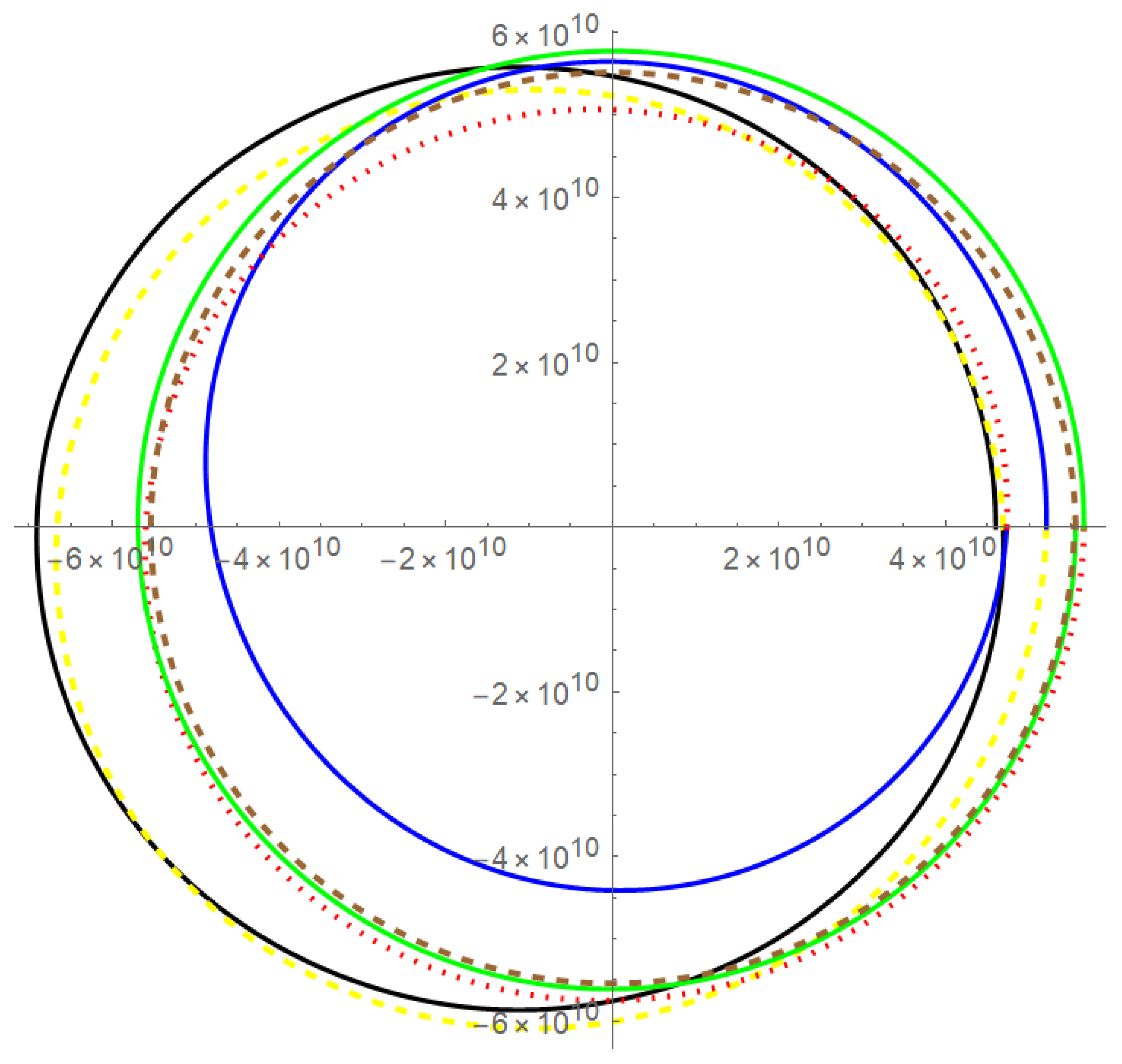
The algebraic approach may give either positive or negative estimates for the cosmological constant. Letting $\mathsf{\Lambda }=2.5\times {10}^{-43}$, we obtain the following polar plot (Figure 3) for Mercury’s trajectory using the numerical solution to Ode (28).

Figure 3. Mercury’s trajectory using Ode (28) with $\mathsf{\Lambda }={\mathsf{\Lambda }}_{+}=2.57\times {10}^{-43}$.

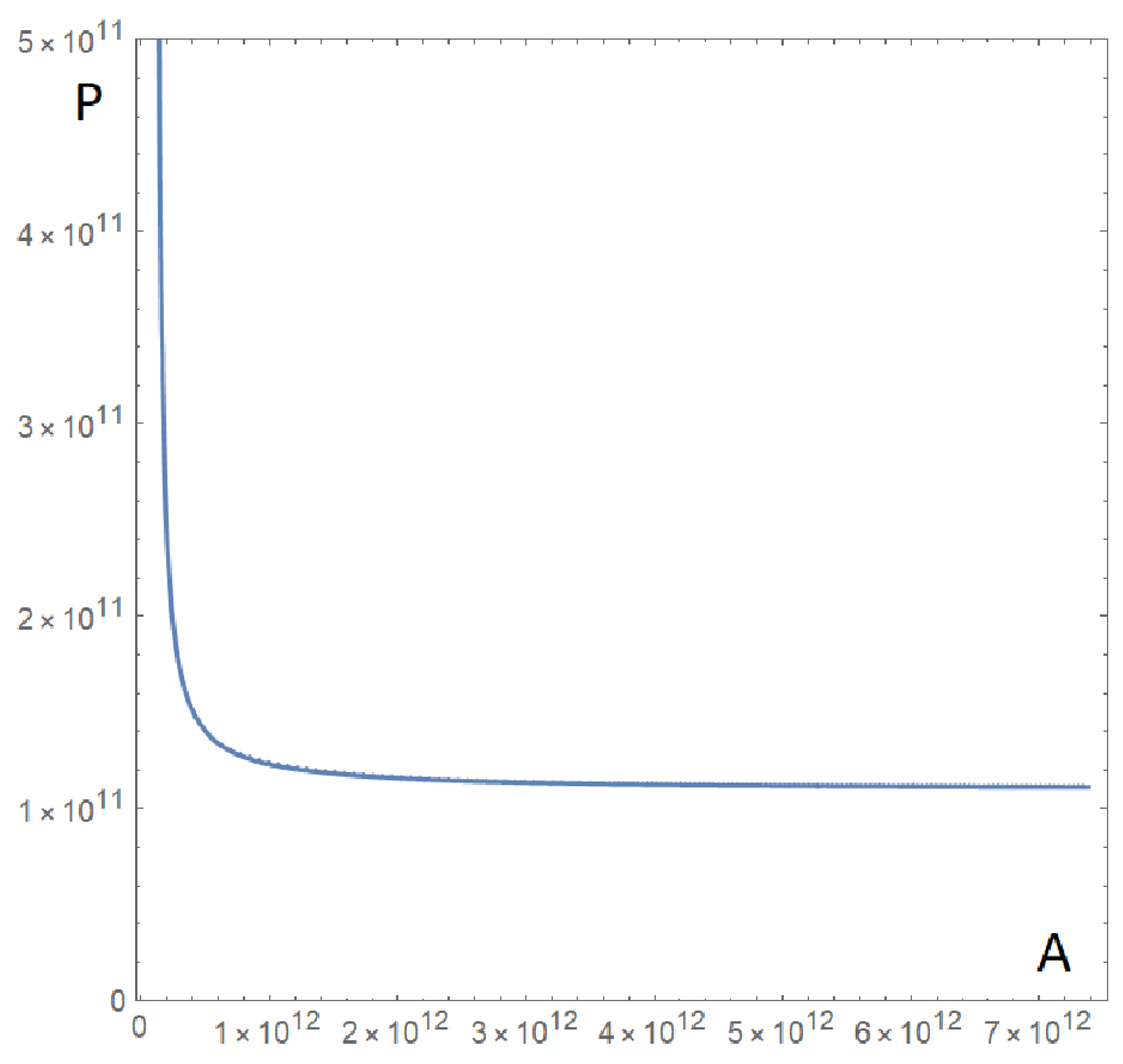
After many calculations to obtain $\mathsf{\Lambda }$ estimates, we found the following interesting fact. Number $\delta$ in Equation (72) was very close to $\delta =1/2953$ for all planets in the solar system. The mean of these values was

$$\delta =0.000338609988014895212199968489565.$$

This implies that

$$\frac{\sqrt{6}K\left(\frac{A-P}{P(A\delta -1)}\right)}{\sqrt{\gamma \left(\delta -\frac{1}{A}\right)}}=\frac{2K\left(\frac{2(A-P)\mu }{2(2A+P)\mu -A{c}^{2}P}\right)}{\sqrt{1-\frac{2\mu (2A+P)}{A{c}^{2}P}}},\mu =GM.$$

(93)

That is, the planets are related to Curve (93) in the $A-P$ plane. This allows for us to predict the value of the aphelion given the the perihelion and vice versa. Indeed, if we are given the aphelion, we simply solve transcendental Equation (93) for the perihelion. On the other hand, the fact that $\delta$ is almost a constant tells us that $\mathsf{\Lambda }$ defined by (79) must indeed be a constant !. This justifies the name ’cosmological constant’; see Figure 4.

Figure 4. Curve (93).

7.2. Second Solution Method

Let

$$F\left(u\right)=-u^3+\frac{3AP-2A\gamma -2P\gamma }{2AP\gamma }{u}^2-\frac{3AP(A+P)\beta }{2\gamma }u-\frac{3AP\beta }{2\gamma },\beta =\frac{c^2\mathsf{\Lambda }}{3L^2}.$$

(94)

Let us introduce the following notations:

$$d_0=-\frac{3AP\beta }{2\gamma },d_1=-\frac{3AP(A+P)\beta }{2\gamma },d_2=\frac{3AP-2A\gamma -2P\gamma }{2AP\gamma }$$

(95)

For a positive $\mathsf{\Lambda }$, the cubic $d_0+d_{1}u+d_2{u}^2-u^3=0$ has two small real roots of opposite signs. For a negative $\mathsf{\Lambda }$, we have only one positive real root, and the two other roots are imaginary and small in magnitude. This allows for us to perform the approximation

$$F\left(u\right)\approx u^2\left(\frac{d_2^4+3d_1{d}_2^2+2d_0{d}_2+d_1^2}{d_2^3+2d_1{d}_2+d_0}-u\right).$$

(96)

Then, hard Ode (58) is replaced with easy ode

$${\left(\frac{du}{d\varphi }\right)}^2=\frac{2\gamma }{3}\left(u-\frac{1}{A}\right)\left(\frac{1}{P}-u\right)\left(\frac{d_2^4+3d_1{d}_2^2+2d_0{d}_2+d_1^2}{d_2^3+2d_1{d}_2+d_0}-u\right)$$

(97)

so that, in view of (64),

$$\begin{array}{ccc}{T}_{\mathsf{\Lambda }}\hfill & \approx & 2\sqrt{\frac{3}{2\gamma }}{\int }_{1/A}^{1/P}\frac{du}{\sqrt{\left(u-\frac{1}{A}\right)\left(\frac{1}{P}-u\right)(\delta -u)}},\hfill \\ \delta \hfill & =& \frac{d_2^4+3d_1{d}_2^2+2d_0{d}_2+d_1^2}{d_2^3+2d_1{d}_2+d_0}\hfill \end{array}$$

(98)

The required equation to estimate the $\mathsf{\Lambda }$ is then

$$2\sqrt{\frac{6A}{\gamma (A\delta -1)}}K\left(\frac{A-P}{P(A\delta -1)}\right)=\frac{4K\left(\frac{2GM(A-P)}{A{c}^{2}P-2GM(A+2P)}\right)}{\sqrt{1-\frac{2GM(A+2P)}{A{c}^{2}P}}}.$$

(99)

For Mercury data, the estimated value using (99) is ${\mathsf{\Lambda }}_{+}=6.51\times {10}^{-52}.$ For Pluto, ${\mathsf{\Lambda }}_{-}=-2.83\times {10}^{-52}$. For data [25]$P=46005766800,A=69818681600$, the estimated value using Formula (99) is $\mathsf{\Lambda }=-3.52\times {10}^{-51}.$

7.3. Third Approach

We may proceed quite differently in order to estimate the $\mathsf{\Lambda }$ value. Let $u_{\mathrm{app}}\left(\varphi \right)$ be some approximate solution to I.V.P. (27), for example, $u=u_{\mathrm{trigo}}.$ Then, replacing u with $u_{\mathrm{app}}$ in (58) gives

$$\mathsf{\Lambda }\left(\varphi \right)=f\left(\varphi \right):=\frac{L_0^2{u}_{\mathrm{app}}\left(\varphi \right){}^2\left(\begin{array}{c}3AP\left(\left(A{u}_{\mathrm{app}}\left(\varphi \right)-1\right)\left(P{u}_{\mathrm{app}}\left(\varphi \right)-1\right)-AP{u}_{\mathrm{app}}^{\prime }{\left(\varphi \right)}^2\right)-\\ 2\gamma \left(A{u}_{\mathrm{app}}\left(\varphi \right)-1\right)\left(P{u}_{\mathrm{app}}\left(\varphi \right)-1\right)\left(AP{u}_{\mathrm{app}}\left(\varphi \right)+A+P\right)\end{array}\right)}{A^2{c}^2{P}^2\left(A{u}_{\mathrm{app}}\left(\varphi \right)-1\right)\left(P{u}_{\mathrm{app}}\left(\varphi \right)-1\right)\left((A+P)u_{\mathrm{app}}\left(\varphi \right)+1\right)}.$$

(100)

Then, we take

$${\mathsf{\Lambda }}_{\mathrm{integral}}=\mathsf{\Lambda }(A,P)=\frac{1}{T_0}{\int }_{-T_0/2}^{T_0/2}{f}^{\prime }\left(\varphi \right)d\varphi .$$

(101)

See Table 5 for the different $\mathsf{\Lambda }$ estimates.

Table 5. $\delta$ value in Equation (72).

Mercury	$\delta$ = 0.000338609961092532513876607325187
Venus	$\delta$= 0.000338609978670453457775396666207
Earth	$\delta$ = 0.000338609983781427330631896843727
Mars	$\delta$ = 0.000338609988303106856661478518689
Jupiter	$\delta$ = 0.000338609994578505351780356447122
Saturn	$\delta$ = 0.000338609995748851561048198277604
Uranus	$\delta$ = 0.000338609996456062380901924635523
Neptune	$\delta$ = 0.000338609996709698414518729947531
Pluto	$\delta$ = 0.000338609996793419042605127744494

Predicted value for ${\mathsf{\Lambda }}_{+}$:

$$\begin{array}{c}\mathrm{Arithmetic} \mathrm{Mean}:{\mathsf{\Lambda }}_{+}=2.87\times {10}^{-44}.\hfill \\ \mathrm{Geometric} \mathrm{Mean}:{\mathsf{\Lambda }}_{+}=1.25\times {10}^{-52}\hfill \end{array}$$

(102)

Predicted value for ${\mathsf{\Lambda }}_{-}$:

$$\begin{array}{c}\mathrm{Arithmetic} \mathrm{Mean}:{\mathsf{\Lambda }}_{-}=-7.25\times {10}^{-44}.\hfill \\ \mathrm{Geometric} \mathrm{Mean}:{\mathsf{\Lambda }}_{-}=-1.01\times {10}^{-52}\hfill \end{array}$$

(103)

Confidence interval for Table 6:

Table 6. Estimation of the cosmological constant using the second and third approaches.

Planet	${\mathsf{\Lambda }}_{+}$	${\mathsf{\Lambda }}_{-}$	${\mathsf{\Lambda }}_{\mathbf{integral}}$
Mercury	$2.58\times {10}^{-43}$	$-1.02\times {10}^{-47}$	$4.18351\times {10}^{-37}$
Venus	$6.34\times {10}^{-49}$	$-6.51\times {10}^{-43}$	$5.54028\times {10}^{-38}$
Earth	$1.05\times {10}^{-49}$	$-4.26\times {10}^{-45}$	$1.45838\times {10}^{-38}$
Mars	$4.0\times {10}^{-51}$	$-5.35\times {10}^{-45}$	$-2.22584\times {10}^{-39}$
Jupiter	$3.33\times {10}^{-53}$	$-2.46\times {10}^{-55}$	$-2.62516\times {10}^{-41}$
Saturn	$5.08\times {10}^{-55}$	$-3.45\times {10}^{-60}$	$-2.53073\times {10}^{-42}$
Uranus	$2.8\times {10}^{-55}$	$-5.33\times {10}^{-59}$	$1.42783\times {10}^{-43}$
Neptune	$4.13\times {10}^{-56}$	$-2.00\times {10}^{-59}$	$2.13098\times {10}^{-44}$
Pluto	$1.38\times {10}^{-56}$	$-8.303\times {10}^{-60}$	$3.78788\times {10}^{-45}$

$\begin{array}{ccc}\mathsf{\Lambda }& {\mathsf{\Lambda }}_{+}& {\mathsf{\Lambda }}_{-}\\ \mathsf{\Delta }\mathsf{\Lambda }& \left\{{-1.3\times 10}^{-43}{,1.9\times 10}^{-43}\right\}& \left\{{-4.8\times 10}^{-43}{,3.3\times 10}^{-43}\right\}\end{array}$

8. Analysis and Discussion

We obtained the estimated values for the cosmological constant, and we compared our results with that obtained in [25]. The nonlinear differential equation in [25] taking into account the cosmological constant reads

$${\left(\frac{du}{d\varphi }\right)}^2=\frac{2GM}{c^{2}u{\left(\varphi \right)}^2}\left(u\left(\varphi \right)-\frac{1}{A}\right)\left(\frac{1}{P}-u\left(\varphi \right)\right)\left(d_0+d_{1}u\left(\varphi \right)+d_{2}u{\left(\varphi \right)}^2-u^3\left(\varphi \right)\right),$$

(104)

where

$$\begin{array}{c}{d}_0=\frac{c^2\left(A^2\left(c^{2}P-2GM\right)+AP\left(c^{2}P-2GM\right)-2GM{P}^2\right)}{2AGMP\left(A{c}^2\mathsf{\Lambda }P(A+P)+6GM\right)}\mathsf{\Lambda }.\hfill \\ \\ d_1=\frac{c^2(A+P)\left(A^2\left(c^{2}P-2GM\right)+AP\left(c^{2}P-2GM\right)-2GM{P}^2\right)}{2AGMP\left(A{c}^2\mathsf{\Lambda }P(A+P)+6GM\right)}\mathsf{\Lambda }.\hfill \\ \\ d_2=\frac{c^2}{2GM}-\frac{1}{A}-\frac{1}{P}.\hfill \end{array}$$

(105)

In the case when $\mathsf{\Lambda }=0$ the exact solution is

$$u\left(\varphi \right)=\frac{c^2}{6GM}+\frac{2c^2}{GM}\wp \left(t+t_0;g_2,g_2\right),$$

where

$$\begin{array}{c}{g}_2=g_2=\frac{A^2{c}^4{P}^2-6A^2{c}^{2}GMP+12A^2{G}^2{M}^2-6A{c}^{2}GM{P}^2+12A{G}^2{M}^{2}P+12G^2{M}^2{P}^2}{12A^2{c}^4{P}^2}.\hfill \\ \\ g_3=g_3=\frac{\left(A{c}^2-6GM\right)\left(c^{2}P-6GM\right)\left(A{c}^{2}P-3AGM-3GMP\right)}{216A^2{c}^6{P}^2}.\hfill \\ \\ t_0={\wp }^{-1}\left(\frac{GM}{2c^2}\left(\frac{1}{P}-\frac{c^2}{6GM}\right);g_2,g_2\right)\hfill \end{array}$$

The solution is periodic, and its period is given by

$$\begin{array}{c}T=\frac{4K\left(\frac{2GM(A-P)}{A{c}^{2}P-2GM(A+2P)}\right)}{\sqrt{1-\frac{2GM(A+2P)}{A{c}^{2}P}}}.\hfill \end{array}$$

In [25] authors use the following data:

$$P=45997620600,A=69820729300.$$

(106)

The perihelion shift for these data is 42.9825 arc-sec/century. The value in [25] was =42.9817 arc-sec/century. On the other hand, for the data in [25],

$$P=46001260500,A=69817089400.$$

(107)

The perihelion shift for these data is 42.9814 arc-sec/century. The value in [25] is 42.9805 arc-sec/century. The authors in [25] used the data

$$P=46010448900,A=69807901000.$$

(108)

For these data, the perihelion shift is 42.9784 arc-sec/century. The value in [25] is =42.9776 arc-sec/century.

Using Mercury data in Table 2, we obtain a perihelion shift of 42.9815 arc-sec/century.

In the case when $\mathsf{\Lambda }\ne 0$, cubic $d_0+d_{1}u+d_2{u}^2-u^3=0$ has two roots very close to zero. Then, we may use the approximation

$$d_2{u}^2+d_{1}u+d_0-u^3\approx \left(\frac{d_0\left(d_2^2+d_1\right)}{d_2^3+2d_1{d}_2+d_0}+\frac{\left(d_1^2+d_2^2{d}_1+d_0{d}_2\right)}{d_2^3+2d_1{d}_2+d_0}u+u^2\right)\left(\frac{d_2^4+3d_1{d}_2^2+2d_0{d}_2+d_1^2}{d_2^3+2d_1{d}_2+d_0}-u\right)$$

(109)

For example, let $\mathsf{\Lambda }=-{10}^{-56}$, $P=46005766800,A=69818681600$ as in [25]. We have:

$$\begin{array}{cc}{d}_0+d_{1}u+d_2{u}^2-u^3=\hfill & (u-3.6156749990681577\times {10}^{-25})\hfill \\ \hfill & (u+3.6156749990680067\times {10}^{-25})\hfill \\ \hfill & (0.0003386099606939169-u).\hfill \end{array}$$

(110)

On the other hand, the right-hand side of (109) is written as

$$(u-3.6156749990681577\times {10}^{-25})(u+3.6156749990680067\times {10}^{-25})(0.00033860996069391686-u)$$

(111)

Using these facts and taking into account that

$$\begin{array}{c}\frac{1}{u^2}\left[\frac{d_0\left(d_2^2+d_1\right)}{d_2^3+2d_1{d}_2+d_0}+\frac{\left(d_1^2+d_2^2{d}_1+d_0{d}_2\right)}{d_2^3+2d_1{d}_2+d_0}u+u^2\right]\hfill \\ \approx \frac{1}{A^2}\left[\frac{d_0\left(d_2^2+d_1\right)}{d_2^3+2d_1{d}_2+d_0}+\frac{\left(d_1^2+d_2^2{d}_1+d_0{d}_2\right)}{d_2^3+2d_1{d}_2+d_0}·\frac{1}{A}+\frac{1}{A^2}\right]:=N\hfill \end{array}$$

(112)

hard Ode (104) may be replaced with easy ode

$${\left(\frac{du}{d\varphi }\right)}^2=D\left(u\left(\varphi \right)-\frac{1}{A}\right)\left(\frac{1}{P}-u\left(\varphi \right)\right)\left(\frac{d_2^4+3d_1{d}_2^2+2d_0{d}_2+d_1^2}{d_2^3+2d_1{d}_2+d_0}-u\left(\varphi \right)\right).$$

(113)

The exact solution to Ode (113) is

$$u\left(\varphi \right)=\frac{1}{P}+\frac{3(P-A)(\delta P-1)}{P(A\delta P-2A+P)\left(1+\frac{12AP}{D(A\delta P-2A+P)}\wp (t;g_2,g_3)\right)},$$

(114)

where

$$\begin{array}{c}D=\frac{2GMN}{c^2},\hfill \\ \delta =\frac{d_2^4+3d_1{d}_2^2+2d_0{d}_2+d_1^2}{d_2^3+2d_1{d}_2+d_0}.\hfill \\ \\ g_2=\frac{D^2\left(A^2{\delta }^2{P}^2-A^2\delta P+A^2-A\delta P^2-AP+P^2\right)}{12A^2{P}^2}.\hfill \\ \\ g_3=\frac{D^3(A\delta P+A-2P)(A\delta P-2A+P)(2A\delta P-A-P)}{432A^3{P}^3}.\hfill \end{array}$$

(115)

Solution (113) is periodic, and its period equals

$$T_{\mathsf{\Lambda }}=2{\int }_r^{\infty }\frac{1}{\sqrt{4x^3-g_{2}x-g_3}}=2\sqrt{\frac{P}{D(\delta P-1)}}K\left(-\frac{A-P}{A(P\delta -1)}\right),$$

(116)

where r is the greatest real root to cubic $4x^3-g_{2}x-g_3=0$. Observe that

$$4x^3-g_{2}x-g_3=\left(x+\frac{D\left(A\right(1+P\delta )-2P)}{12AP}\right)\left(x+\frac{D\left(P\right(1+A\delta )-2A)}{12AP}\right)\left(x-\frac{D(2AP\delta -A-P)}{12AP}\right).$$

(117)

The required equation to determine $\mathsf{\Lambda }$ is

$$2\sqrt{\frac{P}{D(\delta P-1)}}K\left(\frac{A-P}{A(1-P\delta )}\right)=T:=\frac{4K\left(\frac{2GM(A-P)}{2GM(2A+P)-A{c}^{2}P}\right)}{\sqrt{1-\frac{2GM(2A+P)}{A{c}^{2}P}}}$$

(118)

The authors in [25] gave the predicted values ${\mathsf{\Lambda }}_{-}=-{10}^{-55}$ and ${\mathsf{\Lambda }}_{+}={10}^{56}$ for the data

$$P=46005766800,A=69818681600.$$

(119)

On the other hand, the predicted values for $\mathsf{\Lambda }$ solving (118) for data (119) are

$${\mathsf{\Lambda }}_{+}=3.0849194019988974\times {10}^{-45}\mathrm{and}{\mathsf{\Lambda }}_{-}=-1.8381582529562642\times {10}^{-45}$$

(120)

Now, using the method in previous sections, we obtained the following estimates for Data (119) in [25]

$${\mathsf{\Lambda }}_{+}=1.024\times {10}^{-47}\mathrm{and}{\mathsf{\Lambda }}_{-}=-2.58\times {10}^{-43}$$

(121)

Lastly, for the other planets, the estimates for $\mathsf{\Lambda }$ by solving (118) are summarized in Table 7:

Table 7. Theoretical values for $\mathsf{\Lambda }$.

Planet	${\mathsf{\Lambda }}_{+}$	${\mathsf{\Lambda }}_{-}$
Mercury	$3.09\times {10}^{-45}$	$-1.83\times {10}^{-45}$
Venus	$2.64\times {10}^{-48}$	$-2.56\times {10}^{-47}$
Earth	$1.46\times {10}^{-47}$	$-2.12\times {10}^{-46}$
Mars	$8.71\times {10}^{-48}$	$-7.56\times {10}^{-32}$
Jupiter	$9.98\times {10}^{-49}$	$-1.885\times {10}^{-33}$
Saturn	$8.01\times {10}^{-50}$	$-2.74\times {10}^{-51}$
Uranus	$2.23\times {10}^{-51}$	$-1.99\times {10}^{-50}$
Neptune	$2.18\times {10}^{-37}$	$-9.1\times {10}^{-51}$
Pluto	$3.68\times {10}^{-51}$	$-4.66\times {10}^{-36}$

Confidence interval for Table 7:

$\begin{array}{ccc}\mathsf{\Lambda }& {\mathsf{\Lambda }}_{+}& {\mathsf{\Lambda }}_{-}\\ \mathsf{\Delta }\mathsf{\Lambda }& \left\{{-1.1\times 10}^{-37}{,1.6\times 10}^{-37}\right\}& \left\{{-5.5\times 10}^{-32}{,3.8\times 10}^{-32}\right\}\end{array}$

The different previous approaches show that the cosmological constant takes different values, both positive and negative, which leads to establishing that the static cosmological model is unstable and antisymmetric. Due to the difference in the perihelion for each planet, the cosmological constant is different for each one, which implies that the trajectory of the planets must be antisymmetric, that is, elliptical.

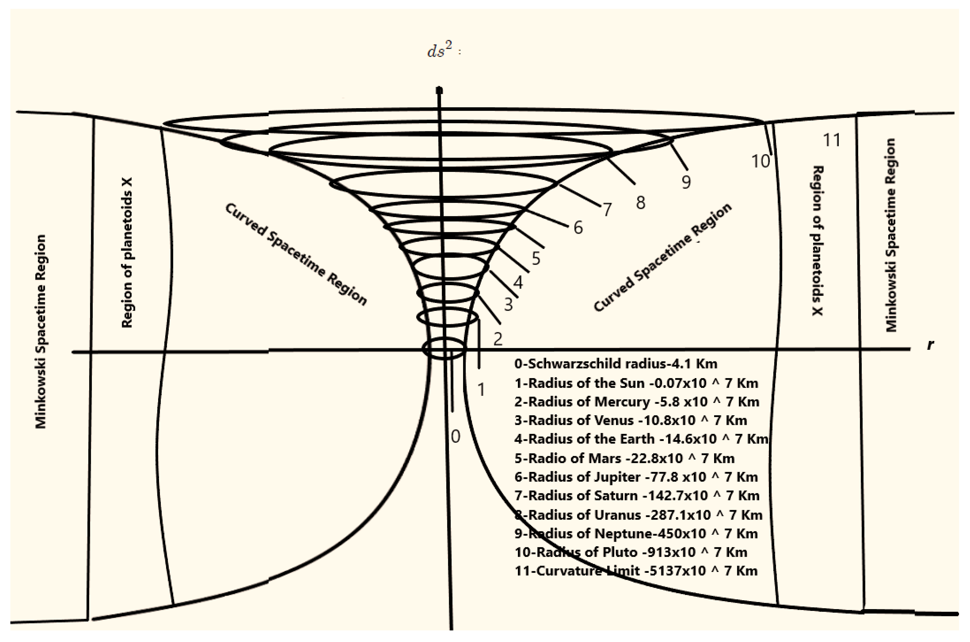
The Schwarzschild radius for the Sun is $r_S=\frac{2GM}{c^2}=2.7$ km. Taking into account the cosmological constant, the Schwarzschild radius is obtained by solving the following cubic equation for r.

$$1-\frac{1}{3}{r}^2\mathsf{\Lambda }-\frac{2GM}{c^{2}r}=0.$$

(122)

Solving (122), we obtain that $r_{S\mathsf{\Lambda }}=4.1$ km. Both radii are inside the Sun.

The region of spacetime due to the gravitational field of the Sun is obtained from

$$1-\frac{1}{3}{r}^2\mathsf{\Lambda }-\frac{2GM}{c^{2}r}=1,$$

(123)

from where $r_{lim}=5.1\times {10}^{10}$ Km = 340 UA.

Between the planet Pluto and the edge of the curved space, an area of the curved spacetime region originates that allows for, in Schwarzschild’s cosmological model, predicting the existence of new planets (planetoids X). Among those catalogued planets are: Kuiper, whose distance to the Sun is 30 AU; Quaoar, 43.4 AU; Makameke, 45.8 AU; Sedna, 88.5 AU; Eris, 98.3 AU; and V774104, 103 AU.

This limit was calculated for the cosmological constant obtained for Mercury $\mathsf{\Lambda }=6.56145\times {10}^{-38}{\mathrm{m}}^{-2}.$

After the boundary of the curved spacetime, a region of Minkowski plane spacetime originates.

From Schwarzschild’s stationary cosmological model (Figure 5), it follows that the planets are in the region of spacetime curved due to the Sun; therefore, each planet follows a stationary geodesic trajectory. All of the above are represented in the following graph.

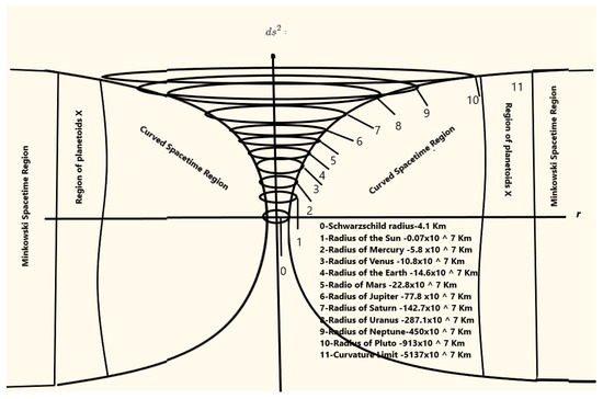
Figure 5. Schwarzschild’s cosmological model.

The static cosmological model of Schwarzschild, the cosmological constant according to the results obtained in Table 4 and Table 6, which were obtained by different approaches, shows that, in the planetary system, the cosmological constant is unstable. In order to understand this effect of instability in the static cosmological model, it is necessary to take into account the effects of the acceleration due to the Big Bang until the current static state is reached.

Lastly, the instability effect of the cosmological constant leads to the fluctuation of the limit radius of the curved spacetime, affecting the stability of the curvature region.

9. Conclusions

In this work, the equation of Einstein’s general theory of relativity for vacuum was solved. Taking into account the cosmological constant, the nonlinear differential equation that describes the movement of the planets was constructed and exactly solved.

Solving the inverse problem, different theoretical estimates were obtained to calculate the value of the cosmological constant. The obtained results were compared with those of other authors, both theoretical and experimental. In the Schwarzschild cosmological radius $r_{S\mathsf{\Lambda }}=4.1$ km, and the radius limit of the curvature of the gravitational field of the solar system $r_{lim}=5.1\times {10}^{10}$ Km = 340 UA were obtained, and the existence of several regions was discovered, which were classified into: planetary curvature region, exoplanet curvature region, and the prediction region of the existence of new exoplanets.

The proposed methodology can be of great interest to astronomers, cosmologists, nonlinear physics researchers, and all those interested in the study of the universe.

References

- Einstein, A. Die Feldgeichungen der Gravitation. Sitzungsber. Preuss. Akad. Wiss. 1915, 844–847. Available online: https://ui.adsabs.harvard.edu/abs/1915SPAW.......844E/abstract (accessed on 11 July 2022).
- Einstein, A. Die Grundlage der allgeminen Relativitatstheorie. Ann. Phys. 1916, 49, 769. [Google Scholar] [CrossRef]
- Schwarzschild, K. Ueber das Gravitattionsfeld eines Massenpunktes nach der Einsteinschen theorie. Preuss. Ak. Wiss. Sitzungsber 1916, 189–196. [Google Scholar]
- Urbain J -J Le verrier. Annales De L´observatoire de paris; Nabu Press: Warsaw, Poland, 1859. [Google Scholar]
- Eddington, A.S. The total eclipse of 1919 May 29 and the influence of gravitation on light. Observatory 1919, 42, 119–122. [Google Scholar]
- Kasner, K. Geometrical theorems on Einstein’s cosmological equations. Am. J. Math. 1921, 43, 217–221. [Google Scholar] [CrossRef]
- Pinzón, J.E.; Salas, A.H.; Castillo, J.E. Non-static solutions of the Einstein equation in the vacuum. Int. J. Math. Comput. Sci. 2022, 17, 439–445. [Google Scholar]
- Pinson, K.H.E. Kasner solution and the causality principle in the relativistic theory of gravitation. Theor. Mat. Phys. 1991, 89, 1236–1238. [Google Scholar] [CrossRef]
- Pinson, K.H.E. Nonstatic solutions of Kazner type in the relativistic theory of gravitation. Theor. Mat. Phys. 1992, 91, 449–451. [Google Scholar] [CrossRef]
- Robertson, H.P. Relativistic Cosmology. Rev. Mod. Phys. 1933, 5, 62–90. [Google Scholar] [CrossRef]
- Walker, A.G. On Milne´s Theory of world structure. Proc. Lond. Math. Soc. 1936, 42, 90–127. [Google Scholar]
- Friedmann, A. Uber die Krummung des Raumes. Zeitschrift für Physik 1922, 10, 377–386. [Google Scholar] [CrossRef]
- Georges, L. Un univers homogène de masse constante et de rayon croissant rendant compte de la vitesse radiale des nébuleuses. Ann. Soc. Sci. Bruxelles 1927, A47, 49–59. [Google Scholar]
- Einstein, A. Cosmological Considerations in the General Theory of Relativity. Sitzungsber. Preuss. Akad. Wiss 1917, 1, 142–152. [Google Scholar]
- De Sitter, W. On Einstein’s theory of gravitation and its astronomical consequences: Third paper. Mon. Not. R. Astron. Soc. 1917, 78, 3–28. [Google Scholar] [CrossRef]
- Edwin, H. A Relation Betwewn Distance and radial velocity Among Extra-Galatic Nebulae. Proc. Natl. Acad. Sci. USA 1929, 15, 168–173. [Google Scholar]
- Eddington, A.S. The Expanding Universe; Cambridge University Press: Cambridge, UK, 1993. [Google Scholar]
- Eddington, A.S. On the Instability of Einstein’s Spherical World. Mon. Not. R. Astron. Soc. 1930, 90, 668–678. [Google Scholar] [CrossRef]
- Einstein, A. Prinzipielles zur allgemeinen Relativitätstheorie. Ann. Phys. 1918, 55, 241–244. [Google Scholar] [CrossRef]
- Tartaglia, A. Testing General Relativity. arXiv 2015, arXiv:1503.00920. [Google Scholar]
- Wilhelm, K.; Dwivedi, B.N. Secular perihelion advances of the inner planets and asteroid Icarus. New Astron. 2014, 31, 51–55. [Google Scholar] [CrossRef]
- Salas Salas, A.H.; Castillo Hernandez, J.E.; Restrepo R., C.E. The Jacobi elliptic functions and their applications in the advance of mercury’s perihelion. Rev. Mex. Fis. 2015, 61, 392–399. [Google Scholar]
- Roig, F.; Nesvorný, D.; DeSouza, S.R. Jumping jupiter can explain mercury’s orbit. Astrophys. J. Lett. 2016, 820, L30. [Google Scholar] [CrossRef]
- Lorenzo, I. The recently determined anomalous perihelion precession of saturn. Astron. J. 2009, 137, 3615–3618. [Google Scholar]
- Kraniotis, G.V.; Whitehouse, S.B. Compact calculation of the perihelion precession of Mercury in general relativity, the cosmological constant and Jacobi’s inversion problem. Class. Quantum Gravity 2003, 20, 22. [Google Scholar] [CrossRef]
- Gibbons, G.W.; Hawking, S.W. Cosmological event horizons, thermodynamics, and particle creation. Phys. Rev. D 1977, 15, 2378. [Google Scholar] [CrossRef] [Green Version]
- Available online: https://calgary.rasc.ca/orbits.htm (accessed on 11 July 2022).
Publisher’s Note: MDPI stays neutral with regard to jurisdictional claims in published maps and institutional affiliations. |
© 2022 by the authors. Licensee MDPI, Basel, Switzerland. This article is an open access article distributed under the terms and conditions of the Creative Commons Attribution (CC BY) license (https://creativecommons.org/licenses/by/4.0/).