Construction and Evolution of Equilibrium Configurations of the Schrödinger–Poisson System in the Madelung Frame

Abstract

We present the construction of ground state equilibrium configurations of the Schrödinger–Poisson (SP) system in the Madelung frame and evolve such configuration using finite volume methods. We compare the behavior of these configurations when evolved within the SP and Madelung frames, in terms of conservation of mass and energy. We also discuss the issues of the equations in the Madelung frame and others inherent to the numerical methods used to solve them.

1. Introduction

The Schrödinger–Poisson (SP) system of equations has recently attracted attention because these equations rule the dynamics of the fuzzy dark matter model (FDM), which proposes that dark matter is an ultralight spinless boson (e.g., [1,2,3,4]). In this model, the Schrödinger equation plays the role of the Gross–Pitaevskii equation for a Bose gas and the Poisson equation provides the potential trap that contains the bosons, whose source is the bosonic gas density itself. The solution of the SP system of equations is the essence of the analyses of this dark matter candidate.

Among the most interesting discoveries within this model is that structures resulting from the evolution of dark matter fluctuations accommodate in density configurations with a core and tail (e.g., [5,6]). The core happens to have the profile of ground state equilibrium configurations of the SP system [7,8], which have been found, in isolated scenarios, to be late-time attractor solutions [9,10].

Now, on the numerical aspect of the simulations based on the numerical solution of the SP system under various astrophysical scenarios, it happens that different numerical methods and approaches are used; see, e.g., [11,12] for reviews on the subject. The various analyses use two main frames for the solution of the SP system, some of them consist of the direct solution of the SP equations, whereas others solve the hydrodynamical Madelung version of the equations [13,14].

Examples solving the SP system include [15], where the first structure formation with ultralight dark matter was examined in [5], where the structure formation within the FDM model using high-resolution simulations receives an important boost; in [16], the oscillation mode spectrum of cores is studied; in [17], the solitonic behavior of cores is revised; the attractor nature of cores is first presented in [10], for the collapse of non-spherical fluctuations; in [18], the star forming structures in FDM filaments is presented; in [19], a zoom in simulation of a galactic halo formation solves the SP equations together with SPH methods; simulations of core mergers are developed in [20,21], where a tidal disruption of FDM subhalo cores is studied.

On the other hand, equations in the Madelung frame have been used to study various other problems. For example, the core-halo mass relations and the possible formation of supermassive black holes [22]; in [23], the existence of vorticity is analyzed in core structures; in [24], local properties of cores are studied, including random motion and collisions; in [25], the Jeans mass shrinking is studied within the scalar field dark matter model; the merger of cores was seen in [26,27]; the equations are solved using the SPH method; in [28], the Schrödinger–Poisson Vlasov–Poisson correspondence is proposed.

Interesting issues emerge in the Madelung frame though. First of all is that Schrödinger equation is cast in an analog fashion to the Euler equations, and therefore the methods developed for the evolution of fluids can be applied. On the other hand, an important drawback of the Madelung frame is that, unlike Euler evolution equations of a compressible fluid, there is not an equation for the balance of energy, and there is no clear Equation of State (EoS) for this quantum fluid analog. Various proposals starting from the Boltzmann equation indicate an EoS, for example, in [25,28], where the SP system is identified with the Poisson–Vlasov system. In our approach below, no EoS or microscopic approach is considered.

Amid the important advances in FDM simulations, the comparison of numerical solutions in the SP and Madelung frames are needed in order to learn about the pros and cons of each approach, and some studies have started in the structure formation scenario [29]. In this paper, we go slightly back and practice a comparison in the simplest of scenarios where the two frames can be compared, namely, the construction and evolution of ground state equilibrium configurations, which, as said before, plays an essential role as galactic cores in the FDM astrophysics. We construct the ground state equilibrium configurations directly on the Madelung frame and evolve them with a code that implements methods used in hydrodynamics in order to compare the dynamics in the two frames.

The paper is organized as follows. In Section 2, we rewrite the SP equations in the Madelung frame and construct the ground state equilibrium solutions. In Section 3, we draw a numerical method suitable for the evolution of these configurations and compare the dynamics of equilibrium configurations in the two frames. Finally, in Section 4, we draw some conclusions.

2. Madelung Transform

We start by writing the SP equations in the FDM regime:

$$i\frac{\partial \mathsf{\Psi }}{\partial t}=-\frac{1}{2}{\nabla }^2\mathsf{\Psi }+V\mathsf{\Psi },$$

(1)

$${\nabla }^{2}V=4\pi {\left|\mathsf{\Psi }\right|}^2,$$

(2)

where $\mathsf{\Psi }$ is the wave function or parameter order of the boson gas and V is the potential trap, which is the gravitational potential sourced by the gas mass itself. These equations are already scaled so that constants are absorbed.

The Madelung transformation defines the wave function in terms of new variables $\rho ,v,S$, $\mathsf{\Psi }=\sqrt{\rho }{e}^{iS}$, and transforms the Schrödinger equation into [13]:

$${\partial }_t\rho +\nabla ·\left(\rho \overrightarrow{v}\right)=0,$$

$${\partial }_{t}S+{\displaystyle \frac{1}{2}}{|\nabla S|}^2+V+Q=0,$$

Equations for $\rho$ and the phase S. By further defining $\overrightarrow{v}=\nabla S$, the SP system is finally transformed into the constrained evolution system

$${\partial }_t\rho +\nabla ·\left(\rho \overrightarrow{v}\right)=0,$$

(3)

$${\partial }_t\overrightarrow{v}+\overrightarrow{v}·\nabla \overrightarrow{v}=-\nabla \left(Q+V\right),$$

(4)

$${\nabla }^{2}V=4\pi \rho ,$$

(5)

where

$$Q=-{\displaystyle \frac{1}{2}}{\displaystyle \frac{{\nabla }^2\sqrt{\rho }}{\sqrt{\rho }}}$$

(6)

is known as the quantum potential. In this frame, $\rho$ is interpreted as the density of a fluid and $\overrightarrow{v}$ as its velocity field. Equations (3) and (4) correspond to the transformed Schrödinger equation, which looks now as a set of two flux balance laws corresponding to the mass conservation and a momentum density balance, analog to Euler equation for a fluid, except by the quantum potential. Notice that unlike the fluid dynamics equations, there is no equation for the balance of an energy nor an equation of state for the fluid, although in some regimes it is possible to identify the fluid with a polytrope with adiabatic index $\mathsf{\Gamma }=2$ [30].

2.1. Diagnostics

The quantities to monitor in both frames are the mass of the system M, and its total energy E = K + W, where K and W are the kinetic and potential energies defined in each frame by

$$M={\int \left|\mathsf{\Psi }\right|}^2{d}^{3}x=\int \rho d^{3}x,$$

(7)

$$\begin{array}{ccc}\hfill K& =& -\frac{1}{2}\int {\mathsf{\Psi }}^{*}{\nabla }^2\mathsf{\Psi }{d}^{3}x\hfill \\ & =& \frac{1}{2}\int \rho |\overrightarrow{v}{|}^2{d}^{3}x+\frac{1}{2}\int {|\nabla \sqrt{\rho }|}^2{d}^{3}x,\hfill \end{array}$$

(8)

$$W=\frac{1}{2}\int {\mathsf{\Psi }}^{*}V\mathsf{\Psi }{d}^{3}x=\frac{1}{2}\int \rho V{d}^{3}x,$$

(9)

That hold when integrated in the spatial domain.

2.2. Ground State Equilibrium Configurations in the SP Frame

We briefly summarize the well-known construction of equilibrium configurations in the SP frame; this is extensively described in, e.g., [7,8]. The first assumption is spherical symmetry, and thus spherical coordinates $(r,\theta ,\varphi ,t)$ are appropriate, so that the wave function depends on the radial coordinate and time $\mathsf{\Psi }=\mathsf{\Psi }(r,t)$. The second assumption is that the wave function depends harmonically of time, that is $\mathsf{\Psi }(r,t)=e^{i\omega t}\psi \left(r\right)$, which ensures ${\left|\mathsf{\Psi }\right|}^2$ is time independent and consequently the gravitational potential as well. Equations (1) and (2) are reduced to

$$\frac{d^2\psi }{d{r}^2}+\frac{2}{r}\frac{d\psi }{dr}=2(V+\omega )\psi ,$$

(10)

$$\frac{d^{2}V}{d{r}^2}+\frac{2}{r}\frac{dV}{dr}=4\pi {\left|\psi \right|}^2,$$

(11)

which define an eigenvalue problem for $\psi \left(r\right)$ provided suitable boundary conditions for the wave function $\psi \left(0\right)={\psi }_c$ and $d\psi /dr\left(0\right)=0$ at the origin, and isolation, which means $\psi (r\to \infty )\to 0$ and $d\psi /dr(r\to \infty )\to 0$. For the gravitational potential, the conditions at the origin are $V\left(0\right)=V_c$, $dV/dr\left(0\right)=0$ and at infinity, a monopolar condition is used $V(r\to \infty )=-M/r$ where $M={\int \left|\psi \right|}^2{r}^{2}dr$. Fulfillment of these conditions imply that for each central value of the wave function ${\psi }_c$ there is a unique eigenfrequency $\omega$ that satisfies the equations. In this sense, one can construct a one parameter family of solutions labeled by the central value ${\psi }_c$.

Finally, unlike excited state solutions, ground state configurations are characterized by the condition that $\psi \left(r\right)$ has no zeroes within the domain of integration, otherwise solutions that satisfy the boundary conditions and has zeroes, are known as excited states (see, e.g., [7,8,9]).

This eigenvalue problem is solved on a discrete domain $r\in [0,r_{max}]$ using the shooting method as described in [8], with a tolerance on the fulfillment of boundary conditions at large radius. The solution for ${\psi }_c=1$ in Figure 1.

2.3. Ground State Equilibrium Configuration in the Madelung Frame

These are spherically symmetric stationary solutions of Systems (3)–(5). For the construction of a stationary configuration we also assume spherical symmetry and use spherical coordinates. The flow is assumed to be stationary, which drops the time derivatives in Equations (3) and (4). The mass conservation reduces to an identity whereas the momentum density balance becomes the equation

$${\displaystyle \frac{d}{dr}}\left(Q\left(r\right)+V\left(r\right)\right)=0,$$

(12)

which can be integrated immediately to obtain a constraint between the gravitational and quantum potentials $Q\left(r\right)+V\left(r\right)=V_0$, where $V_0$ is a constant of integration. Considering the quantum potential is given by (6), this equation is a second-order differential equation for the density $\rho$:

$$\rho ″\left(r\right)=4(V\left(r\right)-V_0)\rho \left(r\right)-{\displaystyle \frac{2{\rho }^{\prime }\left(r\right)}{r}}+{\displaystyle \frac{{\rho }^{\prime }{\left(r\right)}^2}{2\rho \left(r\right)}}.$$

(13)

Notice that substitution of $\rho =\sqrt{\psi }$ in this equation gives the stationary Schrödinger Equation (10) with $\omega =-V_0$. In order to solve this equation, we write it down as a first-order system by defining $u\left(r\right)={\rho }^{\prime }\left(r\right)$. In this way, Equation (13) becomes

$$u^{\prime }\left(r\right)=4(V\left(r\right)-V_0)\rho \left(r\right)-{\displaystyle \frac{2u\left(r\right)}{r}}+{\displaystyle \frac{u{\left(r\right)}^2}{2\rho \left(r\right)}},$$

(14)

$${\rho }^{\prime }\left(r\right)=u\left(r\right).$$

(15)

Now, Poisson Equation (5) is rewritten also as a first order system using the definition of $m^{\prime }\left(r\right)=4\pi r^2\rho \left(r\right)$, which leads to the equations

$$m^{\prime }\left(r\right)=4\pi r^2\rho \left(r\right),$$

(16)

$$V^{\prime }\left(r\right)={\displaystyle \frac{m\left(r\right)}{r^2}}.$$

(17)

The Systems (14)–(17) is the set of equations for equilibrium configurations to be solved; however, notice that their form is not suitable for numerical integration at the origin. Expansion of $u^{\prime }\left(r\right)$ near zero gives:

$$\begin{array}{ccc}\hfill {\displaystyle \underset{r\to 0}{lim}}{u}^{\prime }\left(r\right)& =& {\displaystyle \underset{r\to 0}{lim}}\left(4(V\left(r\right)-V_0)\rho \left(r\right)-{\displaystyle \frac{2u\left(r\right)}{r}}+{\displaystyle \frac{u{\left(r\right)}^2}{2\rho \left(r\right)}}\right)\hfill \\ & =& 4(V_c-V_0){\rho }_c-2{\displaystyle \underset{r\to 0}{lim}}{\displaystyle \frac{u\left(r\right)}{r}}\hfill \\ & =& 4(V_c-V_0){\rho }_c-2{\displaystyle \underset{r\to 0}{lim}}{u}^{\prime }\left(r\right)\Rightarrow \hfill \\ \hfill {\displaystyle \underset{r\to 0}{lim}}{u}^{\prime }\left(r\right)& =& {\displaystyle \frac{4}{3}}(V_c-V_0){\rho }_c,\hfill \end{array}$$

(18)

This is the equation to be solved at the origin instead of (14).

The boundary conditions imposed to these equations are $m\left(0\right)=0$, $\rho \left(0\right)={\rho }_c$, ${\rho }^{\prime }\left(0\right)=u\left(0\right)=0$, and $V\left(0\right)=V_c$, a value that can be arbitrary, and at infinity ${lim}_{r\to \infty }\rho \left(r\right)={\rho }_{\infty }$, ${lim}_{r\to \infty }u\left(r\right)=0$. With these conditions Systems (14)–(18) becomes an eigenvalue problem for the eigenvalue $V_0$.

We numerically integrate the system and approximate the value of $V_0$ using the shooting method, on a discrete domain $r\in [0,r_{max}]$, with the condition of minimizing the value of the function $E\left(V_0\right)=\frac{1}{2}{(\rho (r_{\infty };V_0)-{\rho }_{\infty })}^2+\frac{1}{2}u{(r_{\infty };V_0)}^2$, where ${\rho }_{\infty }$ is a finite small value that helps approximate the solution to zero at infinity with finite numerical precision.

In Figure 1, we show a zoom of the density profile $\rho$ obtained for the solution with central density ${\rho }_c=1$, and ${\rho }_{\infty }=0$ within a small tolerance. Superposed, we show the solution of the eigenvalue Problems (10) and (11) for ${\psi }_c=1$. The eigenvalue of the solution in the two frames is $-V_0=\omega =-0.6922$.

3. Evolution

A further comparison between the solutions in the SP and Madelung frames is the evolution of these configurations. In fact, using one or the other frame motivates the use of different numerical methods. In the SP frame, it is common to use finite difference methods, with a variety of time integrators, explicit or implicit, because Schrödinger equation is dispersive, which prevents the formation of discontinuities. On the contrary, Equation (4) is quasilinear, which may lead to the formation of discontinuities and shocks even for smooth initial data, and then other numerical methods are needed.

In the SP frame, it is possible to show that when solving (1) and (2), the wave function $\mathsf{\Psi }$ oscillates with a frequency that coincides with $\omega$ obtained from the solution of the eigenvalue problem of Equations (10) and (11). Nevertheless, in the Madelung frame, there are no equivalent diagnostics.

A very important aspect is the differentiation of the wave function $\mathsf{\Psi }$, since in general, it can be considered for an equilibrium configurations as a smooth function. On the other hand, in the Madelung framework, some of the variables are not even continuous. We can see this from the definition of S, namely the argument of the function $\mathsf{\Psi }$, which is not defined at the origin, and therefore, for all cases where S is not spatially constant, it will lead to initial data with discontinuous velocities that will tend to produce shock waves, which do not appear in the SP framework. A discontinuity of the velocity leads to a discontinuity of the density, and consequently, Q and $\nabla Q$ are undefined for the right-hand side of Equation (4). Only in cases where the function S is constant can the evolution lead to a solution, even a weak solution.

We then consider that problems in which SP and Madelung frames can be compared, which need to be those with a constant velocity field. In what follows, we describe a comparison of the evolution of the ground state configuration in each of the frames, accompanied with a description of the respective numerical methods.

To start the evolution, we interpolate the equilibrium solutions from Figure 1, constructed in spherical coordinates into a 3D cubic domain described with Cartesian coordinates $D={[x_{min},x_{max}]}^3$, uniformly discretized with N cells along each direction that defines the numerical domain $D_d=\left\{(x_i,y_j,z_k)\right|x_i=x_{min}+i\mathsf{\Delta }x,y_j=x_{min}+j\mathsf{\Delta }x,z_k=x_{min}+j\mathsf{\Delta }x\}$, $j=0,...,N$, where $\mathsf{\Delta }x=\frac{x_{max}-x_{min}}{N}$ is the spatial resolution along the three directions and $\mathsf{\Delta }t=CFL\mathsf{\Delta }{x}^2$ is the time resolution. In the scenarios explored, the domain $D={[-20,20]}^3$ is used with a resolution $\mathsf{\Delta }x=0.4$ and a Courant number CFL = 0.25.

Once the equilibrium configurations in the SP frame is interpolated into the 3D domain described in Cartesian coordinates, we solve Systems (1) and (2) to evolve the configuration in the SP frame using appropriate numerical methods. Likewise, when the equilibrium configuration constructed within the Madelung frame is interpolate into the 3D domain we solve Equations (3)–(6).

3.1. Evolution in the SP Frame

The wave function evolves according to Schrödinger Equation (1), whereas Poisson Equation (2) is a constraint. For the evolution two methods are common and implemented here: the method of lines (MoL) and the implicit Cranck–Nicholson (CN).

For the MoL, the semi-discrete version of the equations uses finite differences with second-order accurate spatial derivatives in Schrödinger equation:

$$\begin{array}{ccc}\hfill \frac{\partial \mathsf{\Psi }}{\partial t}& =& \frac{i}{2}\frac{{\mathsf{\Psi }}_{i+1,j,k}-2{\mathsf{\Psi }}_{i,j,k}+{\mathsf{\Psi }}_{i-1,j,k}}{\mathsf{\Delta }{x}^2}\hfill \\ & +& \frac{i}{2}\frac{{\mathsf{\Psi }}_{i,j+1,k}-2{\mathsf{\Psi }}_{i,j,k}+{\mathsf{\Psi }}_{i,j-1,k}}{\mathsf{\Delta }{y}^2}\hfill \\ & +& \frac{i}{2}\frac{{\mathsf{\Psi }}_{i,j,k+1}-2{\mathsf{\Psi }}_{i,j,k}+{\mathsf{\Psi }}_{i,j,k-1}}{\mathsf{\Delta }{z}^2}-iV{\mathsf{\Psi }}_{i,j,k}\hfill \end{array}$$

(19)

where ${\mathsf{\Psi }}_{i,j,k}$ is the wave function at point $(x_i,y_j,z_k)\in D_d$ at time $t^n$. We integrate this equation from time $t^n$ to time $t^{n+1}$ using a third-order Runge–Kutta explicit integrator.

The Crank–Nicholson method assumes that the evolution of the wave function from time $t^n$ to time $t^{n+1}$ is constructed as follows

$$\begin{array}{ccc}\hfill {\mathsf{\Psi }}_{i,j,k}^{n+1}& =& \frac{e^{-\mathrm{i}\frac{1}{2}\widehat{H}\mathsf{\Delta }t}}{e^{\mathrm{i}\frac{1}{2}\widehat{H}\mathsf{\Delta }t}}{\mathsf{\Psi }}_{i,j,k}^n\Rightarrow \hfill \\ \hfill \mathrm{i}\frac{{\mathsf{\Psi }}_{i,j,k}^{n+1}-{\mathsf{\Psi }}_{i,j,k}^n}{\mathsf{\Delta }t}& =& \frac{1}{2}\left[\widehat{H}{\mathsf{\Psi }}_{i,j,k}^{n+1}+\widehat{H}{\mathsf{\Psi }}_{i,j,k}^n\right].\hfill \end{array}$$

(20)

where we add the upper label to the wave function indicating the time. We solve for ${\mathsf{\Psi }}_{i,j,k}^{n+1}$ using the alternating direction implicit (ADI) strategy, that splits the application of the Hamiltonian $\widehat{H}=-\frac{1}{2}\left(\frac{{\partial }^2}{\partial x^2}+\frac{{\partial }^2}{\partial y^2}+\frac{{\partial }^2}{\partial z^2}\right)+V$, along each of the three spatial dimensions as follows:

$$\begin{array}{ccc}\hfill \left(1-\frac{\mathrm{i}}{4}\mathsf{\Delta }t\frac{{\partial }^2}{\partial x^2}\right)R_{i,j,k}& =& \left(1+\frac{\mathrm{i}}{4}\mathsf{\Delta }t\frac{{\partial }^2}{\partial x^2}\right){\mathsf{\Psi }}_{i,j,k}^n\hfill \\ \hfill \left(1-\frac{\mathrm{i}}{4}\mathsf{\Delta }t\frac{{\partial }^2}{\partial y^2}\right)S_{i,j,k}& =& \left(1+\frac{\mathrm{i}}{4}\mathsf{\Delta }t\frac{{\partial }^2}{\partial y^2}\right)R_{i,j,k}\hfill \\ \hfill \left(1-\frac{\mathrm{i}}{4}\mathsf{\Delta }t\frac{{\partial }^2}{\partial z^2}\right)T_{i,j,k}& =& \left(1+\frac{\mathrm{i}}{4}\mathsf{\Delta }t\frac{{\partial }^2}{\partial z^2}\right)S_{i,j,k}\hfill \\ \hfill \left(1+\frac{\mathrm{i}}{2}\mathsf{\Delta }tV\right){\mathsf{\Psi }}_{i,j,k}^{n+1}& =& \left(1-\frac{\mathrm{i}}{2}\mathsf{\Delta }tV\right)T_{i,j,k}\hfill \end{array}$$

(21)

where $R_{i,j,k}$, $S_{i,j,k}$, and $T_{i,j,k}$ are auxiliary numbers that store the values of the wave function after applying the derivative operator along each of the spatial directions. Each of the three first equations defines a tridiagonal system of equations when derivatives are discretized:

$$\begin{array}{ccc}& & (-\alpha )R_{i-1,j,k}+(1+2\alpha )R_{i,j,k}+(-\alpha )R_{i+1,j,k}=\hfill \\ & & \left(\alpha \right){\mathsf{\Psi }}_{i-1,j,k}^n+(1-2\alpha ){\mathsf{\Psi }}_{i,j,k}^n+\left(\alpha \right){\mathsf{\Psi }}_{i+1,j,k}^n,\hfill \\ & & (-\alpha )S_{i,j-1,k}+(1+2\alpha )S_{i,j,k}+(-\alpha )S_{i,j+1,k}=\hfill \\ & & \left(\alpha \right)R_{i,j-1,k}+(1-2\alpha )R_{i,j,k}+\left(\alpha \right)R_{i,j+1,k},\hfill \\ & & (-\alpha )T_{i,j,k-1}+(1+2\alpha )T_{i,j,k}+(-\alpha )T_{i,j,k+1}=\hfill \\ & & \left(\alpha \right)S_{i,j,k-1}+(1-2\alpha )S_{i,j,k}+\left(\alpha \right)S_{i,j,k+1},\hfill \\ & & {\mathsf{\Psi }}_{i,j,k}^{n+1}=\frac{1-\beta V_{i,j,k}^{n+1/2}}{1+\beta V_{i,j,k}^{n+1/2}}{T}_{i,j,k},\hfill \end{array}$$

(22)

where $\alpha =\frac{1}{4}\mathrm{i}\frac{\mathsf{\Delta }t}{\mathsf{\Delta }{x}^2}$ and $\beta =\frac{1}{2}\mathrm{i}\mathsf{\Delta }t$, which we solve using forward and backward substitution. Notice that the potential is evaluated at the intermediate time $V^{n+1/2}$, which is important because the potential is time-dependent. We calculate this potential as the average $V^{n+1/2}=\frac{1}{2}(V^{n+1}+V^n)$, where $V^{n+1}$ is calculated by solving System (22) for ${\mathsf{\Psi }}^{n+1}$, then solving Poisson equation for the source $|{\mathsf{\Psi }}^{n+1}{|}^2$ to obtain $V^{n+1}$, going back the time-step, and integrating in time with the averaged potential.

In both MoL and CN methods, the Poisson equation is solved using a multigrid method that uses a two-level V-cycle as in [31]. For the evolution of the equilibrium configuration, we impose a boundary condition consistent with the isolation of the system and use a monopolar boundary condition for the gravitational potential $V_{\partial D}=-M/r_{\partial D}$, where $r_{\partial D}$ is the distance from the origin to a given point of the numerical boundary and M is given by Equation (7).

For the wave function, we implement a sponge that absorbs the modes approaching the faces of the boundary and prevents their reflection. This sponge consists in the addition of an imaginary potential that acts as a sink as described in [8,32]. Briefly, the potential V in (1) is redefined as $V\to V+V_{im}$, where V is the solution of (2) and $V_{im}$ is a spherical function with a tanh profile that goes from zero within a sphere containing the region where the interesting physics happens and minus one near the boundary of the domain, which absorbs the wave function if it approaches the boundary.

3.2. Methods for the Madelung Frame

In this frame, the evolution of the system for density $\rho$ and velocity field $\overrightarrow{v}$ is ruled by Equations (3) and (4), whereas again, Poisson Equation (5) is a constraint that has to be fulfilled at each time step during the evolution of density and velocity.

We use a finite volume discretization to solve Systems (3) and (4) following [33]. Essential to the method is the appropriate construction of numerical fluxes and the characteristic structure of the equations, which can be cast in the form

$$\frac{\partial \overrightarrow{u}}{\partial t}+\nabla ·\overrightarrow{F}=\overrightarrow{S},$$

(23)

where $\overrightarrow{u}$ is a vector of conserved variables, $\overrightarrow{F}=[{\overrightarrow{F}}_x,{\overrightarrow{F}}_y,{\overrightarrow{F}}_z]$ a vector of fluxes and $\overrightarrow{S}$ a vector of sources. These elements for Systems (3) and (4) read as follows

$$\begin{array}{c}\overrightarrow{u}=\left[\begin{array}{c}\rho \\ \rho v_x\\ \rho v_y\\ \rho v_z\end{array}\right],{\overrightarrow{F}}_x=\left[\begin{array}{c}\rho v_x\\ \rho v_x{v}_x\\ \rho v_x{v}_y\\ \rho v_x{v}_z\end{array}\right],{\overrightarrow{F}}_y=\left[\begin{array}{c}\rho v_y\\ \rho v_y{v}_x\\ \rho v_y{v}_y\\ \rho v_y{v}_z\end{array}\right]\hfill \\ {\overrightarrow{F}}_z=\left[\begin{array}{c}\rho v_z\\ \rho v_z{v}_x\\ \rho v_z{v}_y\\ \rho v_z{v}_z\end{array}\right],\overrightarrow{S}=\left[\begin{array}{c}0\\ -\rho {\partial }_x(V+Q)\\ -\rho {\partial }_y(V+Q)\\ -\rho {\partial }_z(V+Q)\end{array}\right].\hfill \end{array}$$

(24)

We calculate the numerical fluxes using the HLLE formula [34], according to which the fluxes at the left ${\overrightarrow{u}}_L$ and at the right ${\overrightarrow{u}}_R$ from each intercell boundary, along each of the three Cartesian directions are

$${\overrightarrow{F}}_i={\displaystyle \frac{{\lambda }_{+}{\overrightarrow{F}}_i\left({\overrightarrow{u}}_L\right)-{\lambda }_{-}{\overrightarrow{F}}_i({\overrightarrow{u}}_R+{\lambda }_{+}{\lambda }_{-}({\overrightarrow{u}}_R-{\overrightarrow{u}}_L))}{{\lambda }_{+}-{\lambda }_{-}}},$$

(25)

where $i=x,y,z$, ${\lambda }_{-}$, and ${\lambda }_{+}$ are the approximations of the characteristic velocities, which are calculated as

$${\lambda }_{-}=min(0,{\left(v_i\right)}_L,{\left(v_i\right)}_R),$$

(26)

$${\lambda }_{+}=max(0,{\left(v_i\right)}_L,{\left(v_i\right)}_R).$$

(27)

Notice that with this approach we have not involved the pressure of the fluid; in this case, the pressure-like tensor associated to the quantum fluid within the fluxes. Instead, the gradient of Q is assumed to contribute as a source.

Atmosphere. An inherent ingredient of FV methods is the use of an atmosphere, which is defined as a minimum value of the fluid density, set to ${\rho }_{atm}$. In fluid dynamics it is useful to avoid the divergence of temperature $T=p/\rho$, with p the pressure, which leads to the divergence of all other involved state variables. In our case, there is no pressure, but there is the quantum potential Q in (6), which diverges or is undefined for $\rho =0$, unless ${\nabla }^2\sqrt{\rho }$ compensates the divergence.

Boundary conditions. In order to implement the isolation condition of the system, unlike the sponge in the SP frame, we impose outflow boundary conditions on the fluid variables. In order to solve the Poisson equation, we use a monopolar boundary condition for the gravitational potential $V_{\partial D}=-M/r_{\partial D}$, where $r_{\partial D}$ is the distance from the origin to a given point of the numerical boundary and M is given by Equation (7), and solve using the same multigrid two-level V-cycle method used for the SP frame.

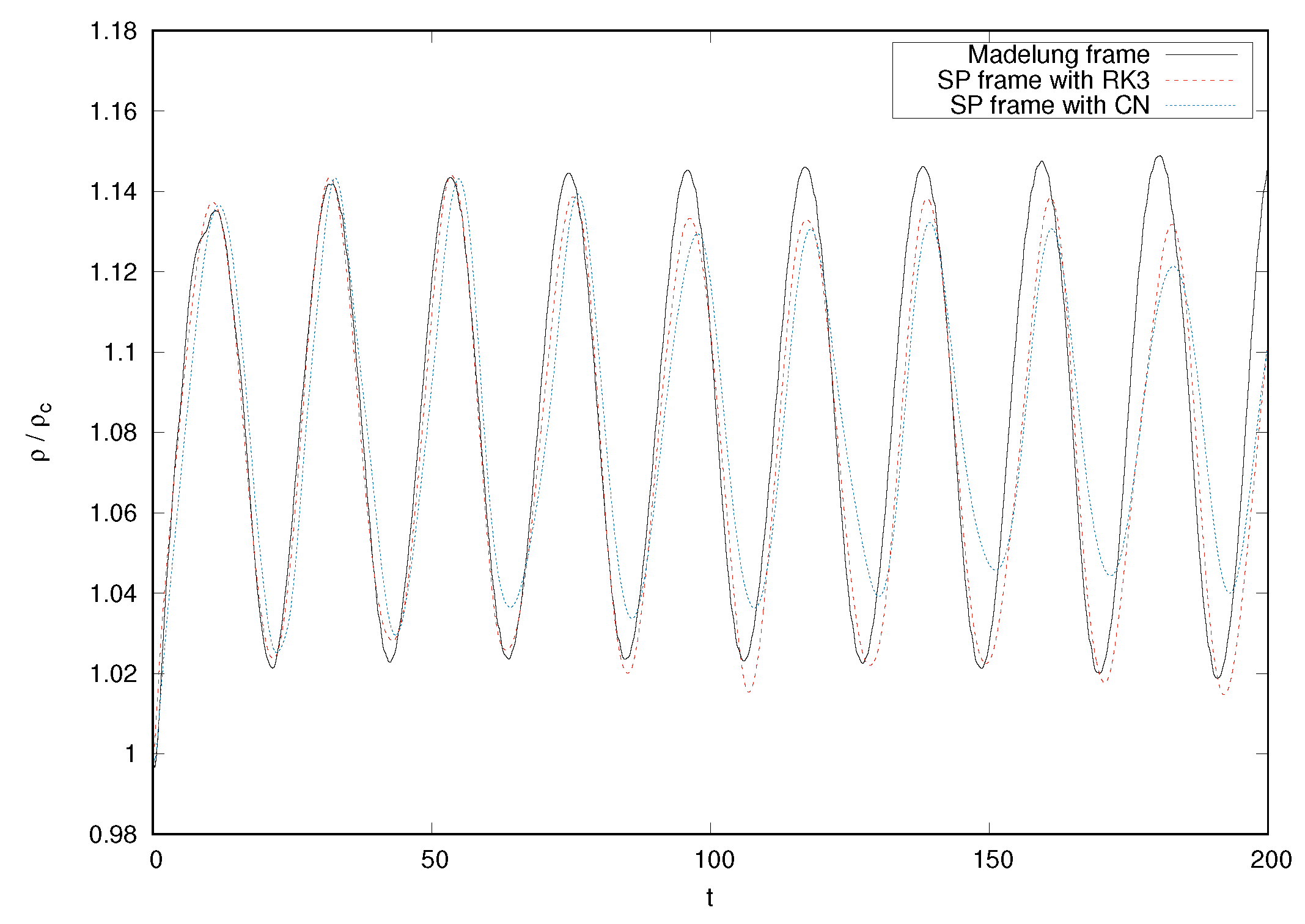
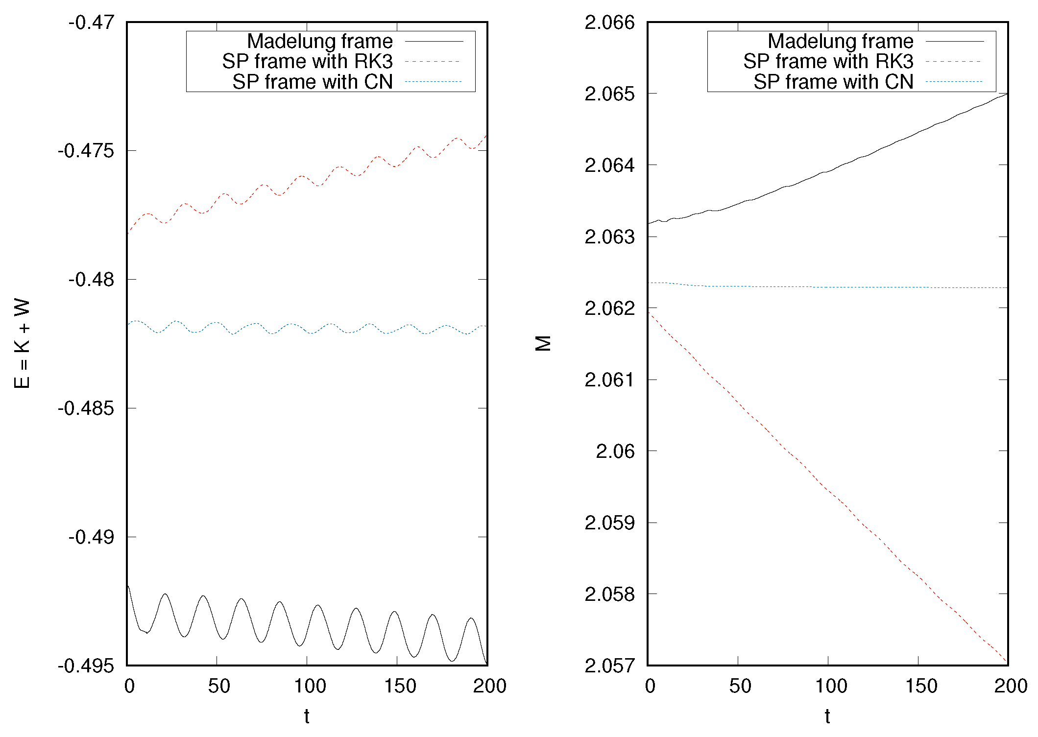
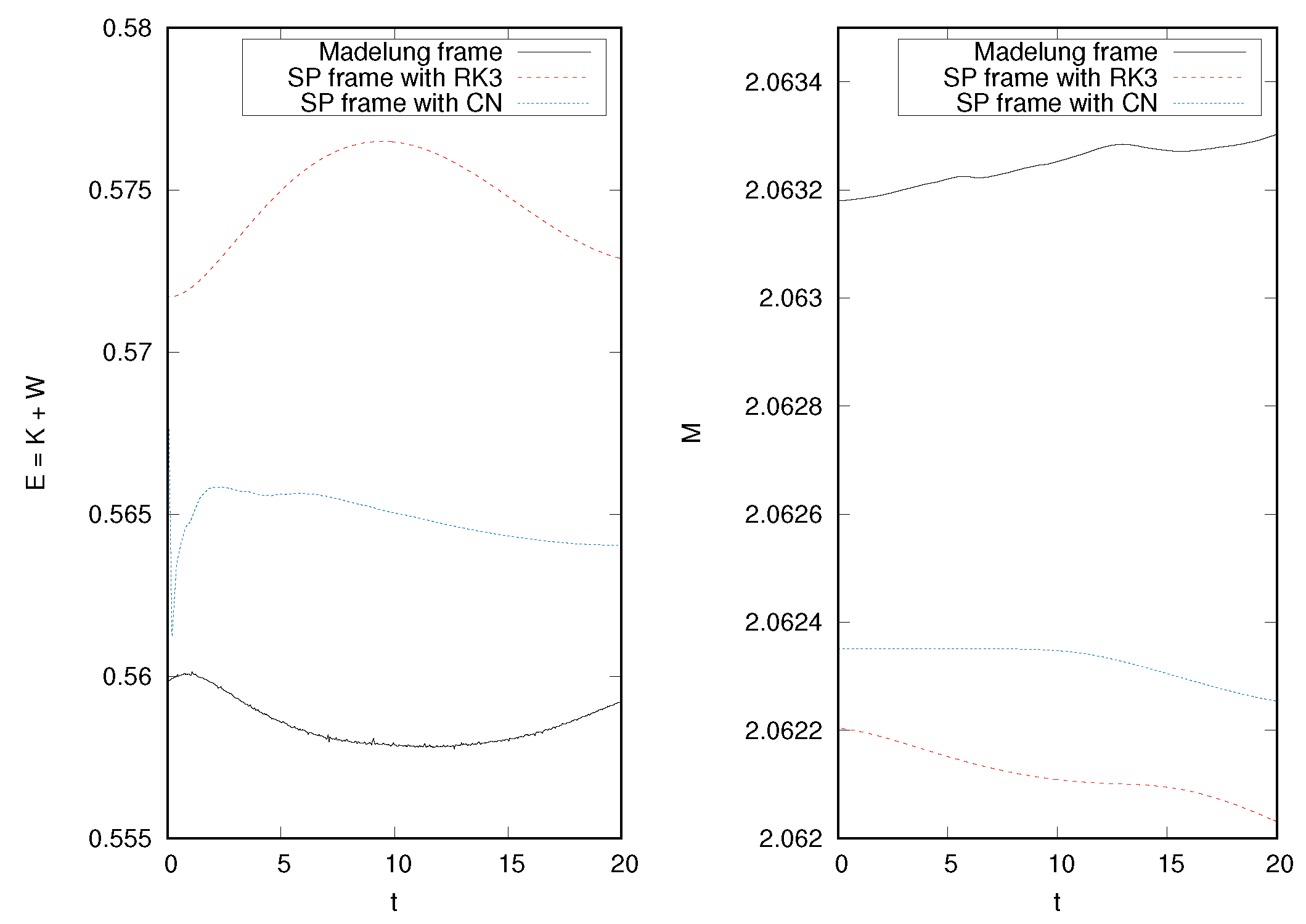
3.3. Evolution of an Equilibrium Configuration

In order to compare the essentials of ground state configurations, we evolve the equilibrium configurations from Section 2 and track their behavior. Using the numerical methods described above for the evolution, we integrate in time the equations for these configurations centered at the coordinate origin, and in Figure 2, we show the central value of the density, $|\mathsf{\Psi }(\overrightarrow{0},t){|}^2$ in the SP frame and $\rho (\overrightarrow{0},t)$ in the Madelung frame. The result indicates that the configuration remains nearly stationary with an oscillation mode consistent with the dominant spherical mode of the configuration with period $T=21.64$ as pointed out in [16] using the SP frame, with both the MoL and CN methods. When using the Madelung frame, there is a reduction in the period in time.

In Figure 3, we show the evolution of the mass M and total energy $E=K+W$ as functions of time. We can see that in the Madelung frame, the mass is slightly bigger than in the SP frame, which is due to the contribution of the atmosphere. Since this atmosphere is of the order of ${\rho }_{atm}\sim {10}^{-8}$, it contributes with a mass of order $M_{atm}\sim {10}^{-3}$. On the other hand, the mass in the SP frame decreases when using the MoL, which is due to the dissipation of the time integration with the explicit RK3 method, whereas the conservation is better when using the CN method, indicating the evolution is closer to unitary.

Concerning the total energy, the values in the two frames disagree due to the difference in mass, which contributes to the gravitational energy W. For this reason, in the Madelung frame the total energy E is smaller than in the SP frame.

3.4. Boosted Equilibrium Configuration

A second comparison is dynamical and corresponds to a boosted equilibrium configuration. For this, we apply an initial velocity $v_x^0=1$ to the equilibrium configuration placed at the initial position (−10, 0, 0), in order to obtain a configuration traveling to the right along the X-axis.

The linear momentum at the initial time is applied to the equilibrium configuration in the SP frame as $\mathsf{\Psi }(\overrightarrow{x},0)={\psi }_0{e}^{\mathrm{i}{v}_x^{0}x}$, where ${\psi }_0$ is the wave function obtained from the solution of eigenvalue Problems (10) and (11). In the Madelung frame, the density is $\rho (\overrightarrow{x},0)={\rho }_0$, and the initial speed is set to $\overrightarrow{v}(\overrightarrow{x},0)=(v_x^0,0,0)$, where ${\rho }_0$ is that of the solution of eigenvalue Problems (14)–(18).

Snapshots of the density are shown in Figure 4. Notice that the maximum of the configuration using the hydrodynamical method in the Madelung frame locates at the appropriate position, since the velocity field is one. On the other hand, the configurations evolved in the SP frame retard with respect to the appropriate location of the maximum density. Nevertheless, this is due to the implementation of the momentum, which actually is a phase, and not a true velocity field at initial time.

In Figure 5, we show the evolution of the total energy E = K + W and the mass M in the two frames. Notice that the energy is well preserved in the two frames and the three methods. The mass decreases in a small fraction in the SP frame that we attribute to the sponge, whereas in the Madelung frame the mass remains relatively constant.

4. Conclusions

We have described the construction of ground state equilibrium configurations of the Schrödinger–Poisson system directly from the equations in the Madelung frame and verified that the solutions in both frames coincide within numerical accuracy.

Since the equations in the Madelung frame are similar to those of a fluid, we implement a simple scheme involving shock capturing methods used in fluid dynamics to simulate the evolution in time. We compare the evolution in SP and Madelung frames using the evolution equilibrium configuration when at rest and when the configuration is boosted.

We find that important limitations of the FV method arise. One of them is the need of an atmosphere used to avoid the singularity of the quantum potential at rarified regions. We notice that this also happens in simple cases within quantum mechanics, for example, in excited states for a particle in a box or a harmonic oscillator potential, where the density has zeroes, then using an atmosphere is needed to avoid the singularity $1/\sqrt{\rho }$ of Q; however, the use of the atmosphere introduces a non-derivable $\sqrt{\rho }$ that will spoil the factor ${\nabla }^2\sqrt{\rho }$ of Q in the intersection between the atmosphere and higher values of $\rho$. It seems that using solely the Madelung frame leads to a dilemma.

This type of problem seems to motivate the use of patches to the FV method, such as in [35], where in low density regions the smoothed particle hydrodynamics (SPH) method is used; or the use the SPH method to solve the evolution equations in the Madelung frame for $\rho$ and $\overrightarrow{v}$ in [27]. It would be interesting to investigate how SPH develops in these simple scenarios.

References

1. Matos, T.; Ureña-López, L.A. Quintessence and scalar dark matter in the Universe. Class. Quantum Grav. 2000, 17, L75–L81. [Google Scholar] [CrossRef] [Green Version]
2. Sahni, V.; Wang, L. New cosmological model of quintessence and dark matter. Phys. Rev. D 2000, 62, 103517. [Google Scholar] [CrossRef] [Green Version]
3. Hu, W.; Barkana, R.; Gruzinov, A. Fuzzy Cold Dark Matter: The Wave Properties of Ultralight Particles. Phys. Rev. Lett. 2000, 85, 1158–1161. [Google Scholar] [CrossRef] [Green Version]
4. Hui, L.; Ostriker, J.P.; Tremaine, S.; Witten, E. Ultralight scalars as cosmological dark matter. Phys. Rev. D 2017, 95, 043541. [Google Scholar] [CrossRef] [Green Version]
5. Schive, H.Y.; Chiueh, T.; Broadhurst, T. Cosmic Structure as the Quantum Interference of a Coherent Dark Wave. Nat. Phys. 2014, 10, 496–499. [Google Scholar] [CrossRef]
6. Mocz, P.; Vogelsberger, M.; Robles, V.H.; Zavala, J.; Boylan-Kolchin, M.; Fialkov, A.; Hernquist, L. Galaxy formation with BECDM I. Turbulence and relaxation of idealized haloes. Mon. Not. R. Astron. Soc. 2017, 471, 4559–4570. [Google Scholar] [CrossRef] [PubMed] [Green Version]
7. Ruffini, R.; Bonazzola, S. Systems of Self-Gravitating Particles in General Relativity and the Concept of an Equation of State. Phys. Rev. 1969, 187, 1767–1783. [Google Scholar] [CrossRef] [Green Version]
8. Guzmán, F.S.; Ureña López, L.A. Evolution of the Schrödinger-Newton system for a self-gravitating scalar field. Phys. Rev. D 2004, 69, 124033. [Google Scholar] [CrossRef] [Green Version]
9. Guzmán, F.S.; Ureña López, L.A. Gravitational Cooling of Self?gravitating Bose Condensates. Astrophys. J. 2006, 645, 814. [Google Scholar] [CrossRef] [Green Version]
10. Bernal, A.; Guzmán, F.S. Scalar field dark matter: Nonspherical collapse and late-time behavior. Phys. Rev. D 2006, 74, 063504. [Google Scholar] [CrossRef] [Green Version]
11. Zhang, J.; Liu, H.; Chu, M.C. Cosmological Simulation for Fuzzy Dark Matter Model. Front. Astron. Space Sci. 2019, 5, 48. [Google Scholar] [CrossRef] [Green Version]
12. Niemeyer, J.C. Small-scale structure of fuzzy and axion-like dark matter. Prog. Part. Nucl. Phys. 2020, 113, 103787. [Google Scholar] [CrossRef] [Green Version]
13. Madelung, E. Quantentheorie in hydrodynamischer Form. Z. Fur Phys. 1927, 40, 322–326. [Google Scholar] [CrossRef]
14. Chavanis, P.H. Mass-radius relation of Newtonian self-gravitating Bose-Einstein condensates with short-range interactions. I. Analytical results. Phys. Rev. D 2011, 84, 043531. [Google Scholar] [CrossRef] [Green Version]
15. Woo, T.P.; Chiueh, T. High-Resolution Simulation on Structure Formation with Extremely Light Bosonic Dark Matter. Astrophys. J. 2009, 697, 850–861. [Google Scholar] [CrossRef] [Green Version]
16. Guzmán, F.S. Oscillation modes of ultralight BEC dark matter cores. Phys. Rev. D 2019, 99, 083513. [Google Scholar] [CrossRef] [Green Version]
17. Bernal, A.; Guzmán, F.S. Scalar field dark matter: Head-on interaction between two structures. Phys. Rev. D 2006, 74, 103002. [Google Scholar] [CrossRef] [Green Version]
18. Mocz, P.; Fialkov, A.; Vogelsberger, M.; Becerra, F.; Amin, M.A.; Bose, S.; Boylan-Kolchin, M.; Chavanis, P.H.; Hernquist, L.; Lancaster, L.; et al. First Star-Forming Structures in Fuzzy Cosmic Filaments. Phys. Rev. Lett. 2019, 123, 141301. [Google Scholar] [CrossRef]
19. Schwabe, B.; Niemeyer, J.C. Deep Zoom-In Simulation of a Fuzzy Dark Matter Galactic Halo. Phys. Rev. Lett. 2022, 128, 181301. [Google Scholar] [CrossRef]
20. Schwabe, B.; Niemeyer, J.C.; Engels, J.F. Simulations of solitonic core mergers in ultralight axion dark matter cosmologies. Phys. Rev. D 2016, 94, 043513. [Google Scholar] [CrossRef] [Green Version]
21. Du, X.; Schwabe, B.; Niemeyer, J.C.; Bürger, D. Tidal disruption of fuzzy dark matter subhalo cores. Phys. Rev. D 2018, 97, 063507. [Google Scholar] [CrossRef] [Green Version]
22. Dawoodbhoy, T.; Shapiro, P.R.; Rindler-Daller, T. Core-envelope haloes in scalar field dark matter with repulsive self-interaction: Fluid dynamics beyond the de Broglie wavelength. Mon. Not. R. Astron. Soc. 2021, 506, 2418. [Google Scholar] [CrossRef]
23. Schobesberger, S.O.; Rindler-Daller, T.; Shapiro, P.R. Angular momentum and the absence of vortices in the cores of fuzzy dark matter haloes. Mon. Not. R. Astron. Soc. 2021, 505, 802–829. [Google Scholar] [CrossRef]
24. Li, X.; Hui, L.; Yavetz, T.D. Oscillations and random walk of the soliton core in a fuzzy dark matter halo. Phys. Rev. D 2021, 103, 023508. [Google Scholar] [CrossRef]
25. Shapiro, P.R.; Dawoodbhoy, T.; Rindler-Daller, T. Cosmological structure formation in scalar field dark matter with repulsive self-interaction: The incredible shrinking Jeans mass. Mon. Not. R. Astron. Soc. 2021, 509, 145. [Google Scholar] [CrossRef]
26. Maleki, A.; Baghram, S.; Rahvar, S. Investigation of two colliding solitonic cores in fuzzy dark matter models. Phys. Rev. D 2020, 101, 023508. [Google Scholar] [CrossRef] [Green Version]
27. Mocz, P.; Succi, S. Numerical solution of the nonlinear Schrödinger equation using smoothed-particle hydrodynamics. Phys. Rev. E 2015, 91, 053304. [Google Scholar] [CrossRef] [Green Version]
28. Mocz, P.; Lancaster, L.; Fialkov, A.; Becerra, F.; Chavanis, P.H. Schrödinger-Poisson-Vlasov-Poisson correspondence. Phys. Rev. D 2018, 97, 083519. [Google Scholar] [CrossRef] [Green Version]
29. Li, X.; Hui, L.; Bryan, G.L. Numerical and perturbative computations of the fuzzy dark matter model. Phys. Rev. D 2019, 99, 063509. [Google Scholar] [CrossRef] [Green Version]
30. Chavanis, P.H. Predictive model of BEC dark matter halos with a solitonic core and an isothermal atmosphere. Phys. Rev. D 2019, 100, 083022. [Google Scholar] [CrossRef] [Green Version]
31. Guzmán, F.S.; Alvarez-Ríos, I.; González, J.A. Merger of galactic cores made of ultralight bosonic dark matter. Rev. Mex. Fis. 2021, 67, 75–83. [Google Scholar] [CrossRef]
32. Guzmán, F.S.; Lora-Clavijo, F.D.; González-Avilés, J.J.; Rivera-Paleo, F.J. Rotation curves of rotating Galactic Bose-Einstein condensate dark matter halos. Phys. Rev. D 2014, 89, 063507. [Google Scholar] [CrossRef] [Green Version]
33. Lin, C.T.; Yeh, J.Y.; Chen, J.Y. High resolution finite volume scheme for the quantum hydrodynamic equations. J. Comput. Phys. 2009, 228, 1713–1732. [Google Scholar] [CrossRef]
34. Thomas, J. Numerical Partial Differential Equations: Conservation Laws and Elliptic Equations; Texts in Applied Mathematics; Springer: New York, NY, USA, 2013. [Google Scholar]
35. Hopkins, P.F. A stable finite-volume method for scalar field dark matter. Mon. Not. R. Astron. Soc. 2019, 489, 2367–2376. [Google Scholar] [CrossRef]
Figure 1. Densities | ψ | 2 and ρ of the ground state equilibrium solution in the SP and the Madelung frames, respectively. In the SP frame, Equations (10) and (11) are solved for the central wave function ψ c = 1 . In the Madelung frame Equations (14)–(18), we use the central density ρ c = 1 . The numerical solution is constructed on a discrete domain with resolution Δ r = 2.5 × 10 4 .
Universe 08 00432 g001
Figure 2. Central density | Ψ ( 0 , t ) | 2 for the solution in the SP frame and ρ ( 0 , t ) in the Madelung frame, as functions of time. This plot shows that the first oscillation mode is similar, although not perfectly equal in the two frames. In the SP frame, the period coincides with that in [16], whereas the period in the Madelung frame shrinks in time.
Universe 08 00432 g002
Figure 3. Evolution of the total energy E = K + W and the mass M of the equilibrium configuration in the two frames.
Universe 08 00432 g003
Figure 4. Snapshots of the density profile every t = 5 time units in the Madelung frame (solid line) and the SP frame (dotted lines).
Universe 08 00432 g004
Figure 5. Evolution of the total energy E = K + W and the mass M as a function of time in the two frames for the boosted configuration.
Universe 08 00432 g005
Publisher’s Note: MDPI stays neutral with regard to jurisdictional claims in published maps and institutional affiliations.